A Work Project, presented as part of the requirements for the Award of a Master Degree in Economics from the NOVA – School of Business and Economics.
Upstream Emissions for Battery Electric Vehicles in the U.S. Fleet Regulation: Environmental Implications and Carbon Dioxide Abatement Potential
Christian Alexander Kubis, 851
A Project carried out on the Master in Economics Program in cooperation with the AUDI AG, under the supervision of:
Professor Antonieta Cunha e Sá, NOVA SBE Professor Maria Clara Costa Duarte, NOVA SBE
Dominik Wöhrle, AUDI AG
06.01.2017
The thesis as presented is based on internal, confidential data and information of the company AUDI AG.
The thesis may only be made available to the first and second examiner as well as to authorized members of the examination boards. Publication and duplication of the thesis – including excerpts thereof – shall not be permitted.
The explicit permission of the author and the company shall be required before the thesis may be inspected by unauthorized parties.
1
Upstream Emissions for Battery Electric Vehicles in the U.S. Fleet Regulation: Environmental Implications and Carbon Dioxide Abatement Potential
Abstract
The U.S. Environmental Protection Agency introduced Carbon Dioxide emission standards for Light-Duty-Vehicles, accounting for emissions associated to electric vehicles for the first time. This affects the incentives of manufacturers like AUDI to comply with the regulations. The purpose of this work is to contribute to a better understanding of the environmental implications of such regulations measured by the estimated total emissions. Therefore, a sensitivity analysis with respect to the most influential parameters is performed. Further, this work provides an indication of the real world CO2 emission savings potential of the regulatory framework, by
examining different manufacturer’s compliance strategies.
Keywords: EPA, Carbon Dioxide, Battery Electric Vehicles, Environmental Impact
1 Introduction
Climate Change is among the most important issues humankind is facing. The main drivers of Climate Change are anthropogenic emissions of Green-House-Gases (GHG). Among these, Carbon Dioxide (CO2) is by far the most significant. After China, the United States of America
are globally the second largest emitter of CO2, responsible for about 16% of total emissions,
which is about is 5556 million metric tons (MMT) of CO2 (EPA, 2016a).
The main source of CO2 emissions is the combustion of fossil fuels for electricity production and
transportation. Within the U.S. transportation sector, Light-Duty-Vehicles (LDVs), consisting of Passenger Cars (PCs) and Light-Duty-Trucks (LDTs), are responsible for about 61% of the GHG emissions (EPA, 2016a). LDVs represent the main part of the U.S. vehicle market.
2 In order to reduce CO2 emissions and comply with supranational climate agreements like the
Paris agreement, many countries force the introduction of new, more efficient and cleaner technologies among all affected industries. In the USA, like in most other relevant markets, the automotive industry has to fulfill ever-tightening efficiency and fuel economy standards. However, it is becoming increasingly complex and expensive to comply with these standards with Conventional Vehicles (CVs) that are gasoline or diesel powered. Mainly these regulations, but also competition and urban mobility, are driving most manufacturers to develop and introduce more electrified vehicle concepts, such as pure Battery-Electric-Vehicles (BEVs). Historically, the emission compliance standards in the U.S. have concentrated only on the usage phase of the vehicles, that is, on tailpipe emissions. From this perspective, BEVs show no CO2
emissions. However, as CO2 is a uniformly mixed pollutant it does not make any difference
where emissions occur. Therefore, it is reasonable to take a more global perspective and consider the emissions that occur in the production process of the energy source as well. For BEVs, this would imply to include emissions from the electricity production. In this context, the American Environmental Protection Agency (EPA) has decided to account for Upstream Emissions (UE) in its current fleet regulation named “2017 and Later Model Year Light-Duty Vehicle Greenhouse Gas Emission and Corporate Average Fuel Economy Standards” (GHG-2) (EPA, 2012a). After a phase in period, the regulation is expected to fully affect most major manufacturers by 2025. The aim of this paper is to study the impact and the environmental potential (with respect to emission savings) of the U.S. legislation for electric cars in the LDV sector in 2025. The analysis is based on a fictive example which is representative for a premium vehicle manufacturer like AUDI. It focuses on CVs and BEVs, as these are predicted to be the main vehicle concepts sold in 2025. Finally, the results are extrapolated to the whole U.S. vehicle market.
3 The rest of the work project is structured as follows: Section 3 explains the UE-Section in the GHG-2 regulation. Section 4 analyzes the impact of four key emission related parameters on the total emission output by means of a sensitivity analysis. Those four key parameters are the electricity grid’s Emission Factor (EF), the electric car’s Electricity Consumption (EC), the Vehicle-Miles-Travelled in the first year of vehicle usage (VMT) and the share of BEVs in a manufacturers vehicle fleet (BEV-Share). The EF and EC are main parameters in the UE-Section, whereas the VMT and BEV-Share are used to determine the total emissions. Section 5 estimates the total CO2 saving potential of UE-Section in the regulation and puts it in context to overall
emissions. Section 6 offers conclusions.
The results of the sensitivity analysis indicate that out of the four key parameters the VMT shows the highest relative impact on emissions. This is because, in contrast to the other factors, it affects the whole fleet and not only the electrified vehicles. The second largest impact is associated with the BEV-Share. Obviously, if the BEV-Share increases, the influence of the EF and EC will also increase. Changes in EF and EC have the same effect on total emissions.
The introduction of the UE-Section in the GHG-2 regulation is increasing the emissions that are considered by the EPA for compliance. This could lead to a compliance gap. Instruments to comply with the regulation would reduce the real world CO2 emissions. In the case of AUDI
USA, this reduction potential is in the order of 90.000 tons CO2 in 2025. Extrapolating this result
to the whole new vehicle market in the U.S. and comparing the results to the total CO2 emissions
shows the limitations of the proposed regulation. This is because the UE-Section of the GHG-2 regulation only affects the electric share of the new vehicles sold in one year. Regulations affecting the whole vehicle stock would most likely be more effective.
4
2 Literature Review
Many sources provide general information on worldwide and U.S. environmental issues and global warming. NASA (2016) offers a basic introduction to the topic. Moreover, the EPA, the International Panel on Climate Change (IPCC), the International Energy Agency (IEA) and others cover the issue. For the automotive sector in the U.S., the EPA, the National Highway Traffic Safety Administration (NHTSA) and the California Air Resource Board (CARB) are the main regulatory drivers in terms of GHG emission reductions.
Knittel (2012) explores the main approaches in order to reduce oil consumption in the transportation sector. Looking at the effects of increasing fuel economy standards, the increased use of non-petroleum-based low-carbon fuels, alternatives to the combustion engine and reduced mileage, he states that the first best policy choice would be putting a price on the externalities, that is, carbon taxes or cap and trade systems. Knittel (2016) emphasizes this point when he argues that without a policy that internalizes the external effects of carbon emissions, it is unlikely that renewable technologies will substitute fossil-fueled alternatives anytime soon. This is because new technologies will make the extraction of fossil fuels cheaper and economically reasonable. In 2015, EPA released its Clean Power Plan (CPP) aiming at reducing the GHG emissions from the electric power sector (EPA, 2015). The CPP is heading in Knittel’s proposed direction but is delegating planning and implementation to the state level.
The EPA first introduced a concept to account for UE in the USA in its first national greenhouse gas emission standards in 2010 (GHG-1), which was published jointly with the NHTSA and covered the Model Years (MY) 2012-2016. As the UE-Section of the GHG-1 was postponed, the regulation under consideration in this work project is the subsequent GHG-2 regulation (GHG-2), which covers the MYs 2017-2025 and was published in 2012. EPA established these UE policies in order to deal with changing emission characteristics and promote the marketing of electrified
5 vehicle concepts. Liven (2015) examined the effectiveness of different demand sided incentives towards electric mobility adoption. Concluding, he advises policymakers to move away from large cash grants towards more investments in infrastructure such as charging facilities. Liebl et al. (2014) offer a deeper insight to energy management in the automotive sector in their German-language technical book “Energiemanagement im Kraftfahrzeug”. They focus on the optimization of CO2 emissions and consumption of conventional and electrified concepts. Their
findings are useful to understand the mechanisms of fleet regulations.
Zivin et al. (2014) contribute tremendously to the understanding of the Emission Factor1. They examine the geographic and temporal variation in the Emission Factors of power plants, showing the implications of marginal emissions for electrified vehicles. They find that the environmental impact of EVs varies tremendously depending on the regional and temporal electricity demand and supply. The U.S. Energy Information Agency (EIA) forecasts the possible trajectories of renewable sources of electricity for different economic and regulatory scenarios in its “Annual Energy Outlook 2016” (EIA, 2016). Asamer et al. (2016) conduct a sensitivity analysis for EC estimation of electric vehicles. They examine the influence of different vehicle parameters on the EC of a BEV, finding that the efficiency of the drive train is the most influential factor. Helms et al. (2010) show the environmental impact of BEVs and Plug in Hybrid Electric Vehicles (PHEVs). They discuss the electric vehicle’s energy efficiency, the electricity generation for electric vehicles and the electric vehicle’s life cycle emissions. They conclude that improvements in the GHG balance highly depend on the energy sources, arguing that EVs have to be charged with additional renewable electricity to be beneficial.
Relating to the effect of improved fuel economy on the mileage driven, De Borger et al. (2016) are measuring the rebound effect with micro data from Danish households. Their results suggest a
1
6 rebound effect in the range of 7.5%-10%. This is at the lower end of other research suggestions. Finally, the International Energy Agency (IEA) shows possible future developments of electric vehicles worldwide in its “Global EV Outlook 2016” (IEA, 2016). Substantial growth in the market is forecasted if the major global temperature target of 2 degrees is to be achieved.
3 CO2 Emissions in the LDV Sector and the U.S. Fleet Regulation
This section explains the sources of CO2 emissions in the LDV sector and provides a brief
description of the regulatory framework introduced by the EPA.
3.1 CO2 Emissions in a Vehicle’s Life-Cycle
The Life-Cycle-Analysis (LCA) divides the occurrence of emissions into four phases along a vehicle’s lifetime: the vehicle production, the production of the vehicles energy source, the usage phase and the recycling of the vehicle. Figure 1 shows the relative breakdown of CO2 emissions
for BEVs and CVs over their life cycle. In the past, regulations on GHG emission standards in the U.S. only concentrated on the usage phase. For CVs, including traditional gasoline and diesel powered cars, by far the largest part of the emissions arises in the usage phase. These emissions are also denoted by Tank-To-Wheel (TTW) emissions. BEVs, on the contrary, have zero emissions on a TTW basis, but show significant emissions in the production phase of the energy source. For BEVs, these Well-To-Tank (WTT) emissions or Upstream Emissions (UE) depend
7 on the CO2 intensity of the electricity production. With the increasing market penetration of
BEVs, the WTT emissions become more relevant. Therefore, the EPA introduced the UE-Section in the GHG-2 regulation and is now using a Well-To-Wheel (WTW) approach for BEVs. The vehicle production and recycling phases are still not considered in the regulation. Therefore, this work focuses on phase two and three of the LCA, namely the TTW and WTT phases.
3.2 Upstream Emissions in the U.S. Fleet Regulation
In Section III.C.2 of the GHG-2 final rule, the EPA introduces “Incentives for Electric Vehicles” (EPA, 2012a). The section is divided into two timeframes, one from MY 2017-2021 and the other from MY 2022-2025.
The aim of EPA’s GHG-2 regulation is to reduce CO2 emissions from the LDV sector. Therefore,
the EPA defines target CO2 emission values for all LDVs. The manufacturers have to comply
with those targets, on average, for the vehicles they sell in a Model Year (MY). This set of vehicles is also denoted by the company’s fleet. The CO2 targets are based on footprint values,
which are vehicle dependent and defined as the area between the vehicle’s tires. Thus, they are a measure of vehicle size. The larger the vehicles are in a company’s fleet, on average, the higher is the target. The specific emission value of a CV is measured on a dynamometer when running a defined driving cycle under defined frame conditions.
For the MY 2017-2021 timeframe, the EPA offers two incentives for BEVs. The first is an uncapped 0 gCO2/mi compliance value for BEVs, thus adopting a TTW approach for BEVs. The
second incentive is implementing a multiplicative factor according to which each BEV accounts for more than one vehicle in the manufacturer’s fleet calculation. This means increasing the BEVs sales volume artificially and, thereby, decreasing a company’s overall compliance value.
8 In the MY 2022-2025 timeframe, the multiplier is no longer provided and EPA capped the 0 gCO2/mi compliance value to a production threshold for each company. This threshold is valid
for the whole period of four MYs. If a company’s BEVs sales volume exceeds this threshold, it has to account for the upstream GHG emissions of the vehicles beyond cap. The analysis in this work concentrates on the MY 2025 because it is expected that, by then, most manufacturers will have exceeded their thresholds. Therefore, they would fully have to account for UE. It is important to note that, within EPA’s Midterm Review, the MY 2022-2025 timeframe is currently in revision.
Equation 1 below shows the EPA’s calculation approach for Upstream Emissions of BEVs. CREE stands for “Carbon Related Exhaust Emissions” and represents the BEV’s net upstream CO2 emissions for the compliance calculation. It is the full net increase in the UE relative to the
UE of a comparable conventional gasoline car. Thus, after estimating the total WTT emissions of a BEV (CREEUP), the WTT emissions of a comparable CV (CREEGAS) are subtracted. The reason for this net accounting is that the UE of CVs have not been considered in the past (EPA, 2012a). As an attempt to achieve comparability, only the net increase in UE is considered.
𝐂𝐑𝐄𝐄 = 𝐂𝐑𝐄𝐄𝐔𝐏 − 𝐂𝐑𝐄𝐄𝐆𝐀𝐒 = 𝑬𝑪
𝑮𝑹𝑰𝑫𝑳𝑶𝑺𝑺∗ 𝑬𝑭 − 𝟐𝟒𝟕𝟖
𝟖𝟖𝟖𝟕∗ 𝑻𝒂𝒓𝒈𝒆𝒕𝑪𝑶𝟐
CREE = Carbon Related Exhaust Emissions (Net increase of WTT emissions relative to comparable CV) CREEUP= Full BEV Upstream (WTT) emissions
CREEGAS= Upstream (WTT) emissions of comparable CV EC = vehicle Electricity Consumption [Wh/km]
GRIDLOSS = 0,935, accounts for grid transmission losses
EF = 0,534, EPA defined electricity greenhouse gas Emission Factor at power-plant [g/Wh]
2478 = estimated grams of upstream greenhouse gas emissions per gallon of gasoline (fuel-factor 1) 8887= estimated grams of CO2 per gallon of gasoline(fuel-factor 2)
TargetCO2 = CO2 Target for comparable conventional vehicle for the appropriate model year
9 The estimation approach involves different parameters. While some are defined by the regulator, such as the Emission Factor, the Gridloss-Factor and the Fuel-Factors, others can be influenced by the manufacturers, such as the BEV’s Electricity Consumption. The BEV’s EC is measured accordingly to the emission values of CVs on the dynamometer.
Applying Equation 1 yields significant emission values for BEVs, ranging around 50 gCO2/km
for a midsize PC in 2025. Therefore, the benefit of every single BEV to CO2 compliance is lower,
compared to a framework without UE. However, BEVs still tend to have better compliance values than comparable CVs (about 130 gCO2/km in this case).
4 The Emissions Estimation Model
In this section, the estimation emissions tool developed is presented. The reference case is defined, and the most important influential parameters are identified. In order to understand the impacts of the different factors on the real world emissions, a sensitivity analysis is performed on four key parameters. Two of those resemble different strategies followed by the manufacturers (BEV-Share and EC). Additionally, the amount of miles travelled per vehicle (VMT), which is determined by demand, plays also an important role. The last key parameter is the EF.
Summarizing, the aim of this section is to evaluate the impact of the four key parameters (EF, EC, VMT, BEV-Share) on total emissions based on a fictive AUDI U.S. new vehicle fleet in 2025. The goal for this sensitivity analysis is not target compliance itself, but to understand how those four parameters affect the overall emissions. Note that all results depend on the frame conditions of the test cycles. Further, note that all data is provided in metric terms.
4.1 Emission Estimation Tool
An emission estimation tool was developed in Microsoft Excel. Figure 2 gives an overview of the theoretical concept of the model. The input values are classified in 5 categories: First,
10 assumptions about the fleet composition of the manufacturer for any specific MY are defined. Starting with the predicted total sales volume, the fleet is divided into car concepts (PC or LDT) and technologies (BEV or CV). A predicted PC-Share and the respective BEV-Share are used for this purpose. The Excel-Tool further distinguishes five vehicle segments (A, B, C, D, S), each for PCs and LDTs. These segments describe different size and luxury categories. They are helpful to make reasonable input assumptions. Predicted segment shares are used to describe the sales volume for each segment. Second, legal emission targets are assigned to every vehicle segment. Following the GHG-2 regulation, the targets depend on the vehicle concept (PC or LDT) and on its specific footprint. Third, information on emission values and Electricity Consumption is needed. For CVs, forecasted gCO2/km values are used, and for
BEVs, forecasted EC values in Wh/km. As a fourth input, the VMT-values have to be defined. The fifth input to the tool is information on the regulatory parameters, such as the EF, the grid-loss factor, among others.
In a first step, the EC values of the BEVs are used to estimate the UE for every vehicle segment. This is undertaken, by accounting for the subtraction of the CVs Upstream Emissions following EPA (WTT adjusted or CREE in Equation 1), as well as from Real World point of view (full WTT, or CREEUP in Equation 1). For CVs, the tool presents TTW and WTT emissions (calculated as CREEGAS in Equation 1) and the sum of both (WTW). WWT is the real world approach for CVs, because it accounts for TTW emissions and the WTT emissions based on their real TTW emissions.
11 In a second step, the tool calculates the weighted (by sales volumes) average fleet emission values. This is done for three different scenarios (cases): “GHG-2 NO UE”, “GHG-2 UE” and “Real World”. “GHG-2 NO UE” represents a calculation which is only accounting for TTW emissions for all vehicle concepts. In the first timeframe of the GHG-2 regulation, the EPA is using such an approach. “GHG-2 UE” describes the case of a regulation including the UE-Section as the EPA introduced it for the second timeframe of the GHG-2 standards. It includes the UE of BEVs, but reduces them by the UE of a comparable CVs (see Equation 1). This value corresponds to the compliance value for the MY 2025. “Real World” accounts for all occurring emissions, that is, a full WTW consideration for all vehicle technologies. Note that these three scenarios are just different ways to account for emissions. Of course, what matters to the environment are only the real world emissions. Therefore, the sensitivity analysis in this section is done for the real world emissions.
In a third step, for each vehicle segment the total real world emission output for the whole fleet in one year can be estimated in tons of CO2. To achieve this, the individual values have to be
multiplied by the respective sales volumes and VMT, and summed across all segments. The “Real World” total fleet emissions are used as a reference in all sensitivity analysis performed. A strongly simplified explanation of steps one to three is provided in Figure 3.
Figure 3. Simplified demonstration of calculation approaches for the three different scenarios.
12
4.2 Key Parameters of Upstream Emission Estimation
The following section identifies the four key parameters which are studied in the sensitivity analysis. It also presents their reference case values.
4.2.1 Emission Factor (EF)
As seen in Equation 1 in section 3.1, the Emission Factor (EF) is a multiplicative factor in the UE calculation and provides the carbon intensity of the electricity production in grams of CO2 per
consumed watthour electricity (g/Wh). Therefore, it depends on the composition of the power-generation technologies in the electricity grid. It will be higher for a mainly coal based electricity mix and lower for an energy-mix relying more on renewable sources like wind or solar. Figure 4 shows the relationship between the EF and the net UE, which are calculated according to Equation 1 for a sample BEV. The figure depicts the expected positive relation between EF and UE.
The computation of an appropriate estimate of the EF for electric vehicles is complex. Several aspects have to be considered. Zivin et al. (2014) show that the EF strongly depends on the time of day of vehicle charging. Due to the changing electricity demand during a day, the composition of the supplying power plants also changes. If BEVs, as predicted, charge mostly at night, during off-peak periods, they charge at a different than average EF. Additionally, BEVs are distributed unequally across the different regions of the country. Therefore, Zivin et al. (2014) also show the importance of considering regional differences in the EF. Further, there is a distinction between the average and the marginal approach to the EF. The average EF describes the average CO2
Figure 4. Upstream Emissions for a sample car for different electricity sources and Emission Factors
13 intensity of the grid; the marginal EF shows the emissions for an extra unit of electricity consumed. As additional BEVs would consume an extra amount of energy that would otherwise not be produced, it makes more sense to use a marginal approach.
The EPA’s calculation does account for all these influence factors (EPA, 2012b). The EPA defines the EF in the GHG-2 regulation as the “average electricity GHG emissions factor for the additional electricity demand represented by the EVs and PHEVs that EPA projects will be sold in MYs 2022-2025 and on the road in calendar year 2030” (EPA. 2012a). For the timeframe of the regulation, the EPA suggests an Emission Factor of 0.534 g/Wh. It is the product of a 0.445 g/Wh power plant EF value and a 1.2 feedstock multiplier, which accounts for the emissions associated with extraction, processing and transportation of power plant feedstocks (EPA, 2012a).
However, this calculation was done in 2012, before the Obama administration introduced the Clean Power Plan (CPP). The CPP aims at reducing CO2 emissions from existing power plants
by 32% until 2030 relative to 2005 values (EPA, 2015b). EPA acknowledges that this might significantly decrease the EF. However, for the time being, EPA sticks to the proposed EF of 0.534 g/Wh (EPA, 2016b). In 2016, President Elect Trump announced in his campaign that he plans to support the coal industry and ensure employment in the sector by canceling environmental regulations (NYT, 2016). Therefore, also a stagnation of the EF seems possible. Depending on the implementation of the CPP under President Trump, the EF could either significantly decrease or stagnate. Because of the increasing competitiveness of renewable energy sources, an increase in the EF is unlikely.
14
4.2.2 Electricity Consumption (EC)
The Electricity Consumption (EC) of a BEV can be regarded as the BEV’s equivalent to the CV’s fuel consumption. In Wh/km it tells, how much electric power is needed on average for a one-kilometer ride within the EPA testing cycles. It also accounts for the losses within the vehicle charging process (EPA, 2012a). The EC depends on factors like vehicle size, weight, aerodynamic drag, rolling friction, technical efficiency and auxiliary power demand.
In order to define realistic reference EC values for BEVs in 2025, the improvement potentials of different factors relative to current technologies were determined. Asamer et al. (2016) assess the importance of such factors in order to estimate the Electricity Consumption accurately. They find that the efficiency of the drive train, the rolling friction and the auxiliary power demand are the most important parameters for the estimation. Based on these findings, the focus in this work lies on the efficiency of the drive train components and the rolling friction. The auxiliary power demand, e.g. for radio or lights, is not represented in the testing cycles and can therefore not be included. Figure 5 shows the potential improvements in components and powertrain efficiencies until 2025. The values were gathered in multiple discussions with experts. These improvements in charging, battery losses, converter, motor and transmission efficiencies could in the best case
Figure 5. BEV Powertrain efficiencies and possible improvements until 2025
Figure 6. Effect of drive train efficiency on Electricity Consumption
15 result in a total improvement of a BEV’s efficiency factor from 0.66 to 0.82. Assuming constant vehicle performance (propulsion EC), Figure 6 shows that the total Electricity Consumption of electric vehicles could be decreased by up to 19.5%, depending on the actual efficiency improvements. In fact, in the real world the effect would be even higher because battery capacity and weight could be reduced for constant range. This would lead to a lower propulsion needed. Besides these efficiency gains, also the tires and their rolling friction are expected to improve. According to AUDI estimates, a 1‰ improvement in a BEV’s rolling friction leads to about 3.5% improvement in its EC on average. Assuming a potential improvement of 1-2‰, EC reductions of 3.5% to 7% seem possible.
In total up to 26,5% EC reduction are feasible in the very best case. The EC values for the reference case are based on an analysis of today’s BEV’s Electricity Consumptions, and an adjustment for the best guess of the future development of their efficiency and rolling resistance of 15%. The values are shown in Table 2 in the reference case section. A decrease of 26.5% in the EC requires extreme technological efforts and investments. Considering the economic constraints in the industry, a more conservative forecast of 15% improvement is reasonable.
4.2.3 Vehicle Miles Travelled (VMT)
For the definition of reasonable VMT for the first year of usage, two important assumptions are considered: first, there is no difference in the drive schedule between BEVs and CVs (EPA, 2016b), and second, there is a difference in drive schedule between PCs and LDTs (EPA, 2016c). Estimates of the average PC and LDT VMT, dependent on the vehicles age, are provided using two EPA datasets, one from 2009 and the other from 2012. Further, two different forecasts for yearly mileage increases were used to extrapolate these values to 2025. The first is 0.6% following the EPA Technical Support Document from (EPA, 20012c) and the other is 0.92%
16 according to the Federal Highway Administration’s nationwide Vehicle Travel Outlook (FHA, 2016). The average of the results yields first year mileage forecast of 25.738 km for PCs, and 28.791 km for LDTs for the year 2025.
Further, the VMT is also influenced by an effect commonly referred to as the rebound effect. It describes how drivers respond to improved energy-efficiency of their vehicles (De Borger et al., 2016). It tries to estimate the relation between improved vehicle efficiency and the respective mileage driven. De Borger et al. (2016) find a rebound effect of 7.5%-10%, working with data form Danish households. This is a lower bound of other literature suggestions. EPA suggests a rebound effect of 10% (EPA. 2016c). For a rebound effect of 10%, an increase in a vehicles efficiency of 20% results in a 2% mileage increase. The 10% rebound value takes into account historic as well as more recent research and a trend to declining rebound effects with increasing incomes. For the sensitivity analysis in this work project, the rebound effect is initially set to “0” to derive the pure impact of EC variations. Subsequently, the rebound effect is set to 10% and another sensitivity analysis is executed for the EC. Thus, the interdependencies between the rebound effect and the EC can be examined.
4.2.4 Battery Electric Vehicle Share (BEV-Share)
The last key parameter to be considered in the sensitivity analysis is the degree of electrification in a manufacturer’s fleet. In this work, the “BEV-Share” refers to the share of fully electrified vehicles relative to the whole manufacturer’s fleet. PHEVs will not be considered, as they are predicted to be only bridging technology; they are expected to become obsolete as soon as BEVs become fully competitive, both economically and performance wise (MT, 2015). In its Global EV Outlook 2016, the International Energy Agency (IEA) shows the worldwide development of the EV car stock. In 2015, more than 700.000 BEVs were on the road, surpassing the threshold of
17 half a million for the first time ever. Growth in the past years was stunning, showing annually rates of 84% in 2014 and 77% in 2015 (IEA, 2016). Driven by increasing regulatory requirements (e.g. CO2 emissions or particulate matter) and exceptional technological progress in
the battery technologies, EVs become more and more indispensable for the manufacturers on the one hand and economically reasonable for the consumers on the other hand. In November 2015 AUDI USA announced “to achieve at least 25% of U.S. sales from electric vehicles by 2025” (AudiUSA, 2015). Many other manufacturers plan to increase their EV sales dramatically as well. VW is planning to introduce up to 20 electrified models until 2020 and GM is marketing the first mass market long range BEV, the Chevrolet Bolt, by the end of 2016 (USAToday, 2016). For its Model 3, the pure BEV Company Tesla has more than 400.000 preorders in its books (N-TV, 2016). The rise of electric mobility is likely to continue; however, predictions of the exact pace vary broadly. Therefore, it seems reasonable to assume a share of BEV sales between 20% and 40% by 2025 for premium OEMs like AUDI, considering the manufacturer’s announcements and taking into account the market growth in the recent years. Therefore, a BEV share of 30% is assumed for the reference case.
4.3 Reference Case
This section presents the reference case. Table 1 summarizes the reference case values for the key parameters examined in the sensitivity analysis. Note that EF and EC are inputs to the UE calculation (Equation 1), while mileage and BEV-Share are used to estimate the total emissions in the emission estimation tool.2
2
Equation 1 includes a number of additional parameters that are not subject to the sensitivity analysis. As changes and improvements in the electricity grid are extremely slow and hard to influence, the Gridloss-Factor is assumed constant. Since the sensitivity analysis focuses on real world total emissions, the TargetCO2 in Equation 1 is not relevant for the analysis.
Table 1. Reference Case Values for Key Parameters
18 For confidentiality reasons, all values are fictive. However, they are representative for premium manufacturers like AUDI and reflect reasonable industry expectations. The input parameters are structured as shown in section 4.1. The first input parameter is the AUDI USA fleet composition 2025. It is assumed to have a sales volume of 250.000 vehicles with a PC share of 55%. BEVs represent 30% of the total fleet. The segment shares for PCs and LDTs are shown in Table 2. This table also shows the footprint values, legal targets, CV’s TTW emissions and BEV’s Electricity Consumptions for every segment in the reference case.
Under these assumptions, the total emissions from the “Real World” point of view would be 1.015.676 tons of CO2. This is the amount of total WTW emissions produced by all new vehicles
of the AUDI fleet in 2025. The estimation of was performed as explained in section 4.1.
4.4 Sensitivity Analysis
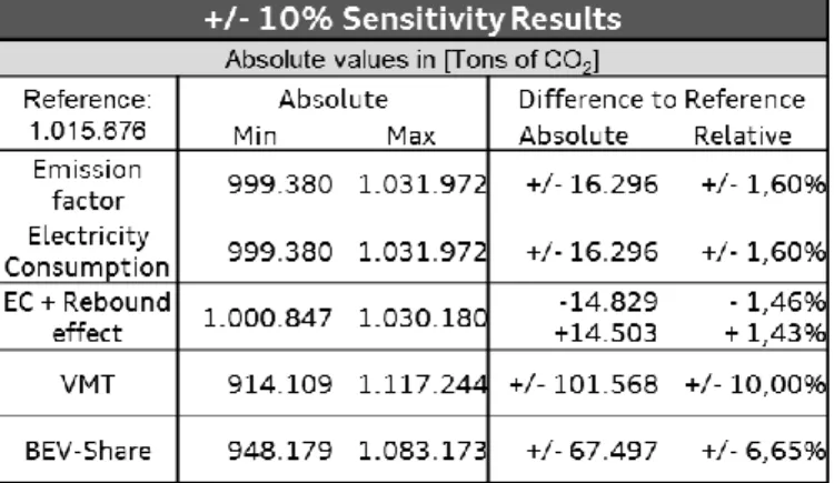
This section presents the results of the sensitivity analysis for the four key parameters identified above. It shows the effect on real world emissions in case manufacturers are willing to modify the fleet characteristics (BEV-Share and EC), or frame conditions change (EF and mileage). The results consider a range of 10% change for each parameter. Table 3 presents an overview of the results.
For a 10% change, the VMT has the highest impact. As the total emissions for 2025 depend on the mileage driven in that year, the VMT enters the model directly and linearly. The VMT affects
19 the emissions of every car in the fleet, regardless of whether it is a BEV or a CV. A 10% change in VMT results in 10% variation in real world emissions. Therefore, the VMT would be the most powerful of the four parameters to decrease overall emissions. However, it is difficult to induce changes in VMT as the consumers determine them. Vehicle manufacturers have limited influence on it. Further, if the VMT decreases, this would also affect the whole U.S. vehicle stock. Therefore, it would have a higher impact on total real world emissions compared to affecting only the new vehicle registrations. The second most influential key parameter is the BEV-Share. The reason for the high contribution of the BEV-Share to real world emissions is the following: Increasing the BEV-Share substitutes CVs for BEVs. From a real world perspective, i.e., including Upstream Emissions for CVs, BEVs emit about 90-120 gCO2/km less than their
conventional counterparts, depending on the vehicle characteristics. Furthermore, with higher BEV-Shares improvements in the EC and the EF would affect more vehicles, and thereby have a greater impact. The BEV-Share is partially in the hands of the manufacturers. While it is subject to a wide range of constraints, it is the manufacturer’s most influential parameter on real world emissions in this context. Changes in the electricity grid Emission Factor and changes in the Electricity Consumption have a relatively small effect on emissions. Both, the EC and the EF enter Equation 1 in the same way (as direct multiplicative factors) and thereby influence the model equally. Changes in the EF are in the hands of the electricity producers and the regulator. When regulators strictly enforce programs to reduce emissions from the electricity-producing sector, emission reductions associated to the LDV sector and many other electricity-consuming Table 3. Sensitivity analysis results
20 industries would follow. If the manufacturers could achieve the same percentage reduction in the Electricity Consumption of their BEVs, it would have the same effect on total emission for the LDV sector. However, it would have no effects on other industries. When also accounting for the rebound effect, results are slightly different. As explained in section 4.2.3, people tend to drive more when the cars get more efficient, and vice versa. Hence, the effect of the EC is partially compensated and thus, smaller than the pure EC’s effect. In the real world, under the assumption of the rebound effect, the effect of the EC on total real world emissions is slightly lower than the effect of changes in the EF. Thus, the EC is expected to have the smallest real world impact of the four key parameters that are tested in this sensitivity analysis.
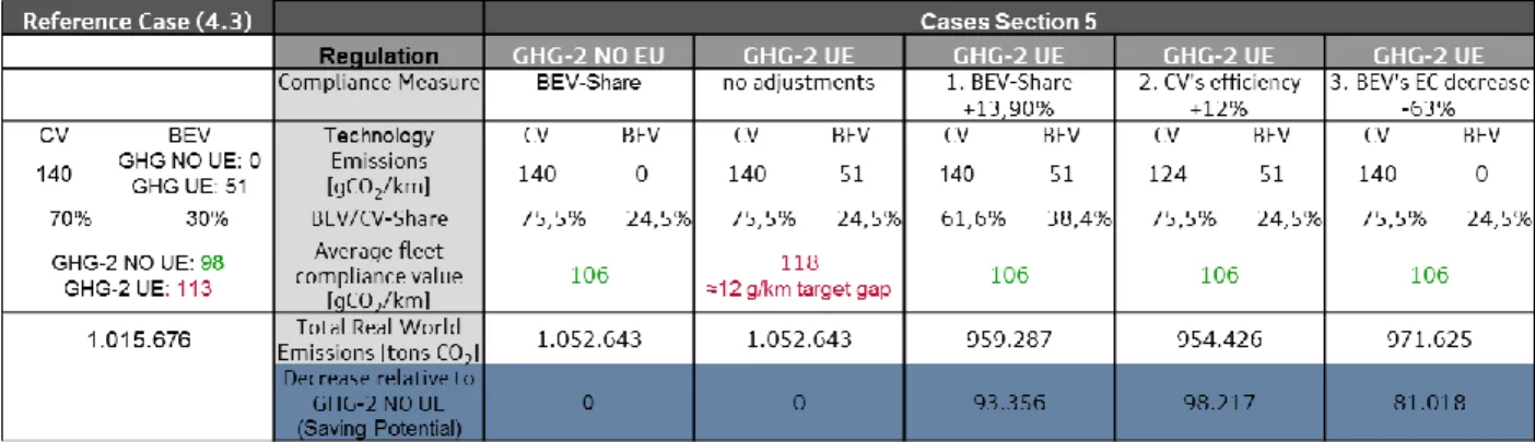
5 CO2 Saving Potential of the UE-Section in the GHG-2 Regulation
In this section, the real world emission reduction potential of the UE-Section in the GHG-2 regulation is estimated. These potentials could arise because of different behavior and decisions of firms in different regulatory scenarios. This section considers two different regulatory scenarios, “GHG-2 NO UE” and “GHG-2 UE” and compares the difference in total real world emissions in case a manufacturer complies with his average fleet target in each of these scenarios. For AUDI this target is predicted to be 106 gCO2/km in 2025. The target does not change within
the scenarios, however, the compliance value of the manufacturer does (because of the accounting for UE). This section examines different instruments to close the emerging target gap and evaluates the respective effects on total real world emissions. Table 4 provides an overview of the steps and instruments.
As seen in first column of Table 4, with the fleet structure form the reference case in 4.3, the manufacturer would easily comply in the “GHG-2 NO UE” case, as the BEV-Share in the reference case is higher than needed for compliance. However, for economic reasons, it is
21 assumed that manufacturers will try to exactly achieve their target and not go beyond. The emission estimation tool shows that a BEV-Share of 24.5% is sufficient to be compliant in the “GHG-2 NO UE” case (column 3). All other input parameters stay as in the reference case. Total emissions in this case would be 1.052.643 tons of CO2. This is the new base value for this
exercise, and the outputs of the following scenarios have to be compared to it to see the regulation’s saving potential.
With this new fleet structure (BEV-Share of 24.5%), the manufacturer would not be compliant in the “GHG-2 UE” framework (column 4). A target gap of 12 gCO2/km emerges, as the
requirements are higher in the “GHG-2 UE” framework. This is because the positive effect of BEVs is lower (51 gCO2/km instead of 0 gCO2/km, in this example). Therefore, the
manufacturers have to react to achieve compliance within the “GHG-2 UE” framework. Three independent potential instruments for compliance are analyzed in the last three columns of Table 4: 1.) increasing the BEV-Share, 2.) increasing the CV’s efficiency and 3.) decreasing the BEV’s EC. For each of these, total real world emissions are calculated and compared to the total real world emissions from the “GHG-2 NO UE” case. The difference is considered the CO2 saving
potential. The results show that total real world reductions because of an increasing BEV-Share (instrument 1) are about 93.400 tons of CO2. If the company would instead increase in the CV’s
22 efficiency (instrument 2), the reductions would be about 98.200 tons of CO2. For decreases in the
BEV’s EC (instrument 3), about 81.000 tons of CO2 could be saved. Note that for changes in the
CV’s efficiency and the BEV’s EC, the effect on real world emissions is partially compensated by the rebound effect.
However, manufacturers do not determine the BEV-Share and the other parameters only because of compliance. There are a many other factors influencing those decisions which are not analyzed in this study. Further, each of these instruments is too extreme to be very likely on its own. Especially the EC improvement is way out of the feasible range defined in 4.2.2. In reality, manufacturers are expected to rather combine the different approaches in order to become compliant. Assuming a 5% improvement of the CV’s efficiency, and a 5% decrease in the BEVs EC, the tool estimates a BEV-Share of 31.6% needed for compliance. This more realistic scenario would lead to reductions in real world fleet emissions of about 93.200 tons of CO2. This is a
reduction potential of 8,85% relative to the emissions from the “GHG-2 NO EU” case.
According to these estimations, the Upstream Emission regulation would lead to emission reductions in the order of 90.000 tons of CO2 for the AUDI new vehicle fleet in 2025, depending
on the instruments used. Under the assumption that AUDI’s fleet composition in 2025 is representative for the U.S. vehicle market, it is possible to extrapolate the saving potential to the whole new vehicle market in the U.S. This is done with the help of AUDI’s predicted market share of 1.61% in 2025. The estimated abatement potential would be 5.738.700 tons of CO2. Note
that an extrapolation by market shares can only provide a rough estimation. It does not account for the different characteristics of the manufacturers in the U.S. market. In order to understand the impact of the regulation, it is interesting to see these values in relation to overall U.S. emissions. Compared to the total emission values of the LDV sector in 2014 of 1060 MMT of
23 CO2 (EPA, 2016a), the regulation could lead to a reduction of 0.55%. Relative to the overall CO2
emissions in the USA of 5556 MMT of CO2 (EPA, 2016a), the potential would be 0.104%.
6 Conclusion
Introducing the UE-Section in the GHG-2 regulation, the EPA increases the share of real world WTW emissions that are included in the regulation. Compliance for the automotive industry becomes more difficult under these conditions. This leads the industry to tackle the CO2
emissions further. These actions do not only help for compliance, but also have real world emission impacts for the fleet sold in a given MY. Within the context of the UE-Section in the GHG-2 regulation, the manufacturer’s most influential instrument to decrease real world emissions is the BEV-Share. Same sized relative changes in the EC have significantly lower impacts. In other words, relative changes in the EC would have to be a lot higher to achieve the same emission reductions compared to changes in the BEV-Share. The EF has the exact same relative impact on real world output as the EC, but it cannot be influenced by the automotive industry directly. The VMT would also be a powerful tool towards real world emission reduction, but it is also very difficult to control, as it is in the hands of the consumers.
The marginal effect of the UE-Section in the GHG-2 regulation on total emission output in 2025 as seen in Section 5 is not a surprise. The effect is cursed to be small, as the section is only affecting a small portion of the new vehicle market, which is roughly 6% of the total vehicle stock on the road. Further, this analysis is only looking at the year 2025. However, regulations like the GHG-2 aim at the reductions in the long term, as they show cumulative effects: as the regulation might drive the manufacturer to increase their electrification share, the benefits could accumulate year by year and make a significant difference in the long run. An extrapolation of the results of the mixed approach in Section 5 to the whole vehicle stock of about 240 million
24 LDVs in the USA can be a first indicator for real world emission effects in the long run. Assuming that the whole U.S. vehicle stock had the characteristics of the mixed approach of Section 5, emission reductions of about 90 million tons of CO2 seem plausible. This is a very
rough estimation, but it can give a hint of the greater impact of such a regulation in the long term. The CO2 reductions could be even higher with more renewable sources of electricity being
online. However, in order to reduce CO2 emissions from the LDV sector in the short and medium
term, also other instruments should be taken into account. One very effective instrument could be decreasing overall mileage for the whole vehicle stock. Achieving this, however, is difficult as the mileage is demand driven and not directly controllable. Still, a potential but controversial instrument could be increasing gasoline taxes.
References
Asamer, Johannes and Anita Graser and Bernhard Heilmann and Mario Ruthmair. 2016.
“Sensitivity analysis for energy demand estimation of electric vehicles.” Transportation
Research Part D, 46 (2016): 182-199.
AudiUSA. 2015. “Audi declares at least 25% of U.S. sales will come from electric vehicles by 2025.” Assessed on 4.12.2016. https://www.audiusa.com/newsroom/news/press-releases/2015/11/audi-at-least-25-percent-u-s-sales-to-come-from-electric-2025. De Borger, Bruno and Ismir Mulalic and Jan Rouwendal. 2016. “Measuring the rebound effect
with micro data: A first difference approach.” Journal of Environmental Economics and
Management, 79 (2016): 1-17.
EIA. 2016. “International Energy Outlook 2016.” U.S. Department of Energy. Washington. EPA. 2012a. “2017 and Later Model Year Light-Duty Vehicle Greenhouse Gas Emission and
Corporate Average Fuel Economy Standards; Final Rule.” FR Vol. 77, No.199, II.
EPA. 2012b. “Regulatory Impact Analysis: Final Rulemaking for 2017-2025 Light-Duty Vehicle Greenhouse Gas Emission Standards and Corporate Average Fuel Economy Standards.” EPA-420-R-12-016.
EPA. 2012c. “Joint Technical Support Document Final Rulemaking for 2017-2025 Light-Duty Vehicle Grenhouse Gas emission Standards and Corporate Average Fuel Economy Standards.” EPA-420-R-12-901.
EPA. 2015a. “Carbon Pollution Emission Guidelines for Existing Stationary Sources: Electric Utility Generating Units; Final Rule.” FR Vol. 80, No. 205, II.
EPA. 2015b. “Factsheet: The Clean Power Plan.” https://www.epa.gov/sites/production/files/ 2015-08/documents/fs-cpp-overview.pdf. Assessed on 20.09.2016.
25 EPA. 2016a. “Overview of Greenhouse Gases.” Assessed on 17.11.2016.
https://www.epa.gov/ghgemissions/overview-greenhouse-gases.
EPA. 2016b. “Proposed Determination on the Appropriateness of the Model Year 2022-2025 Light-Duty Vehicle Greenhouse Gas Emissions Standards under the Midterm
Evaluation.” EPA-420-R-16-020.
EPA. 2016c. “Draft Technical Assessment Report: Midterm Evaluation of Light-Duty Vehicle Greenhouse Gas Emission Standards and Corporate Average Fuel Economy Standards for Model Years 2022-2025.” EPA-420-R-12-901.
FHA. 2016. “Forecasts of Vehicle Miles Travelled (VMT): Spring 2016.” http://www.fhwa.dot. gov/policyinformation/tables/vmt/vmt_forecast_sum.pdf. Assessed on 28.11.2016. Zivin, Joshua S. and Matthew J. Kotchen and Erin T. Mansur. 2014. “Spatial and temporal
heterogeneity of marginal emissions: Implication for electric cars and other electricity-shifting policies.” Journal of Economic Behavior & Organization, 107(2014): 248-268. Helms, Hinrich and Martin Pehnt and Axel Liebich. 2010. „Electric vehicle and plug-in hybrid
energy efficiency and life cycle emissions.” Ifeu – Institut für Energie- und Umweltforschung.
IEA. 2016. “Global EV Outlook 2016.” Paris, International Energy Agency
Knittel, Christopher. 2012. “Reducing Petroleum Consumption from Transportation.” Journal of
Economic Perspectives, 26(1): 93-119.
Knittel, Christopher. 2016. “Will We Ever Stop Using Fossil Fuels?.” Journal of Economic
Perspectives, 30(1): 117-138.
Liebl, Johannes and Matthias Lederer and Klaus Rohde-Brandenburger and Jan-Welm Biermann and Martin Roth and Heinz Schäfer. 2014. “Energiemanagement im Kraftfahrzeug – Optimierung von CO2-Emissionen und Verbrauch konventioneller und elektrifizierter
Automobile.“ Springer Vieweg.
Lieven, Theo. 2015. “Policy measures to promote electric mobility – A global perspective.”
Transportation Research Part A, 82 (2015): 78-93.
MT. 2015.”Rupert Stadler, Audi boss in the eye of an emissions storm.” Assessed on 4.12.2016. http://www.managementtoday.co.uk/exclusive-rupert-stadler-audi-boss-eye-emissions-storm/article/1373946.
NASA. 2016. “Climate change: How do we know?” Assessed on 17.11.2016. http://climate.nasa.gov/evidence/.
N-TV. 2016. “Tesla sammelt Geld für sein "Model 3".“ Assessed on 15.12.2016. http://www.n-tv.de/wirtschaft/Tesla-sammelt-Geld-fuer-sein-Model-3-article17725666.html.
NYT. 2016. “Trump’s Promises Will Be Hard to Keep, but Coal Country Has Faith.” Assessed on 7.12.2016. http://www.nytimes.com/2016/11/28/us/donald-trump-coal
country.html?_r=0.
USAToday. 2016.”Tesla fighters: GM, Toyota strategies diverge.” Assessed on 15.12.2016. http://www.usatoday.com/story/money/cars/2016/05/21/tesla-fighters-gm-toyota-strategies-diverge/84581412/.