Numerical modelling of operational risks for the banking industry

Numerical modelling of operational risks for

the banking industry

R. Barreira, T. Pryer & Q. Tang

Department of Mathematics, Sussex University, UK

Abstract

In Basel II Capital Accord, the Advanced Measurement Approaches (AMA) is stated as one of the pillar stone methods for calculating corporate risk reserves. One of the common yet cumbersome methods is the one known as loss distribution approach. In this article, we present an easy to implement scheme through electronic means and discuss some of the mathematical problems we encountered in the process together with proposed solution methods and further thought on the issues.

Keywords: loss distribution, bottom-up approach, operational risk, Monte-Carlo simulation.

1 Introduction

In Basel II Capital Accord, the use of top-down or bottom-up method to calculate risk provisions are recommended as the ways to model and compute corporate risk value (VaR – values at risk). We mainly discuss the bottom-up approach. For this approach, there are process based models, actuarial models and proprietary models.

The process based model splits banking activities into simple business steps, the management evaluates the situation according to these steps to identify risks. This is mainly a time series type of model. Regressional analysis tools are often used when there are multi-factors in the problem (cf. [1, 2, 5–7]).

The actuarial models or statistics models are generally parametric statistical models. Various statistical fitting techniques are used (see extensive discussions in [3]). In this article, we present an efficient, direct way for this approach and we also discuss some of the technical difficulties that need to be solved.

The advantage of our actuarial model is that once it is set, the model itself will give results very close to historic expected total loss. However, extensive Monte-Carlo disturbance to the multi-parameter model can be made on various levels and simulate a complicated business operation. It can also incorporate features such as management control impact on reduction of losses. We only discuss the general philosophy of algorithm design but not the details of how to implement various technical control issues. Our final program operates in the world-wide-web environment.

The proprietary models are mainly developed by major finance service companies. The approach involves a variety of bottom-up, top-down and qualitative analysis schemes. It is mainly spreadsheets based. It was mentioned in [3] that the currently available proprietary software include Algo OpVantage by Algorithmics Inc, Six Sigma by Citigroup and GE Capital, and Horizon by JP Morgan Chase and Ernest & Young. Interested readers should go to the internet search engines to obtain more information.

2 The modelling approach

In order to describe the loss profile of a corporate entity, it is important to collect the past data from the company. If the company has accumulated enough data over the past three to five years, then we can use the method defined in this section to model the company risk. The method falls into the general category of LDA but without the parts of estimating parameters and fitting to an existing distribution function, the model is based on direct modelling of the existing loss data.

The reason for using direct modelling rather than fitted to an existing probability distribution is as follows:

1) Computational techniques make the handling of thousands of data automatic and instant, it can also highlight many critical issues automatically (such as few observations among some risk classes, very high loss values in a risk class etc) to alert the management in a mechanical manner.

2) The estimate of the loss value and frequency can now be done by Monte-Carlo simulation. When hundreds or thousands of data are involved, the Monte-Carlo simulation of the business operation becomes much more closer to real life situations.

Our discussions are based on real industrial consultancy experience, the modelling problems / challenges mentioned are real world situations. In each subsequent section, we concentrate on one particular issue, we give the background information on why these issues are arising, what is the expectation of the company management and what we can do to build a robust mathematical model.

According to past discussions, it is a common agreement that the risks faced by a company should be classified according to

Company

Business Departments Individual risk events

At the lowest level, it is common now to give a label to each individual risk events (just an example) in the way of

110 corresponding to “Default on payment” 320 corresponding to “Falsified identity”

etc. To simplify the discussion, these events are regarded as probabilistically independent events for the business.

Of course, they can also be treated as dependent events, then the aggregation of different probability distribution functions will be different from what we present now, we postpone the discussion to Section 7.

The business departments within a company will be directly responsible to a number of risk events. It is a common practice not to let different departments to share same risk events. So the structure looks like

Department 1 Department 2 ••• ••• Risk 110 Risk 210 ••• ••• Risk 120 Risk 220 ••• ••• ••• ••• ••• •••

It is common that risk are analysed per risk event and aggregated back to departmental and company level. The labelling of the risks provides a convenient way for the assessment and analysis using internet web forms and programmed algorithm.

2.1 The data collection system

A web based reporting system installed across the business’s offices, departments should provide a reporting form as:

Table 1: Possible risk report form from a web reporting system. Risk No Time reported Loss value Impact Probability

110 02/02/2003 312,227.71 M L

210 03/07/2003 0 L M

300 07/10/2003 536.24 H L The reported event with loss value “0” in the report form is called a “near-miss” event, where an event has happened against the interest of the company and has been observed, but there is no immediate observable money loss. However, it cannot be excluded that hidden loss has happened or will happen. In real life reporting, the front line management should type in the information of Risk number, Time reported and Loss value. The remaining columns should be generated automatically according to the risk number. They are perceptions of the management regarding this particular risk number and are pre-defined in the program.

The meanings of the quantities involved in the table are as follows: • Risk No – an identity number given to the risk event.

• Time reported – the time when the report of the loss is made OR the actual date when this event happened.

• Loss value – the actual recorded value of loss – this may be inconclusive as hidden losses may appear later.

• Impact – the perceived severity of loss for such event should it happens. This could be visible financial losses and/or invisible reputation losses. • Probability – the perceived probability that such event can occur. • Range – the perceived range of loss should such event happens. Usually

this is linked to the Impact column, may not be directly linked to the reported visible loss.

• L=low, M=medium, H=high. They have associated values depending on the circumstances of the company.

For example, for impact, H could mean loss values are between 2m and 5m, M could mean 0.5m to 2m, and L could mean below 0.001m and 0.5m. Particularly small losses below 0.001m may be ignored.

For probability, it is the same, H could mean 20% to 10%, M could be 10% to 4% and L could be 4% to 0.1%.

It is widely agreed that “low impact, low probability” events can be ignored, “High impact, low probability” events have to be modelled separately. That leaves us with the 7 or so remaining categories (various kinds of L, M and H combinations).

2.2 Construction of probability distribution

Based on this reporting system, we can accumulate and sort all data for Risk No 10, for example, we list all loss data in increasing order (here time factor has been ignored, it could also be ordered according to the time when it happens), if the loss observation xj has occurred pj (≥ 1) times, the associated frequency will be pj. The loss observations will be in the following format

Observations for risk No k Loss sum xk1 xk2 … xkS Frequency pk1 pk2 … pks

Remark: The index can be arranged in any convenient order.

We can then construct a probability distribution around each loss value, say

g

_s

(

µ

_s

,

σ

_s

)

where gs is a probability density function,

µ

s is the “assigned” expected loss and

σ

_s is the “assigned” spread of the loss (risk of the loss). The strategy for computing these parameters should be decided by using neighbouring loss data. For example, if loss xs is one of the actual loss observations, to construct the probability distribution

g

_s

(

µ

_s

,

σ

_s

)

, we can use

xs-p < xs-p+1 < … < xs < … < xs+q

to calculate the expected loss and risk. Here loss observations are from the same risk number.

Remark:

1) The distribution function can be normal, gamma or any other appropriate distribution. For example, if normal distribution is used, truncation at 0 (loss values are all regarded as positive) and re-weighting is necessary.

2) The assigned expected loss and assigned spread of the loss will depend on the neighbouring loss values. Different models have different ways of computing.

3) This requires that the parameters are calculated “locally”, eliminating the need for estimating the parameters of the probability distribution. 4) The “localization method” can give large rare loss a large associated

spread (risk), therefore smoothing the probability distribution associated. It will also concentrate sharply where a large number of losses are observed.

The probability loss function can then be constructed using weighted sum, the weight is the frequency of ith _{loss value (the number of times it appeared) over} the total frequency in that risk number.

Remark: It is easy to check that if the loss distribution thus constructed for risk number i is fi, we have

Expectance of [fi]

≈

Expectance of frequency

×

Expectance of Loss Here we do not have equality because of truncation and re-weighting errors. This conforms to the insurance risk modelling principle.

After constructing the probability distribution for losses in each risk number, we can aggregate them by using weighting coefficient

total number of observations in this risk number ---

total number of observations for the whole business

The resulting probability distribution gives the basis of modelling of company risk.

Finally, random perturbations can be given to each loss value and its frequency. The perturbed model will exhibit rather complicated behaviour and resembles to a real business operation. The perturbation pattern can be decided by the company need. After many simulations, an estimated loss interval can be extracted using certain percentage confidence.

3 Give different weights to different years of data

Background: Assuming that the management system is reasonably efficient, gradual improvements will be in place for controlling high / medium impact losses. Considering the delay in time in the management process, it is anticipated that j-year-old data will have less impact on current operation that (j-1)-year-old data for any j.

Solutions: design the program to detect how many observations are there in the past three years, if the observation number is low, do not subdivide the

observations into annual subgroups, treat the 3–5 year data as one group and apply a reduction factor according to how many data in year two, how many data in year two etc.

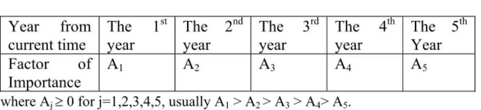
1) Standard approach (there are enough observations): we apply reduction factors as follows

Table 2: Reduction factor. Year from current time The 1st year The 2nd year The 3rd year The 4th year The 5th Year Factor of Importance A1 A2 A3 A4 A5

where Aj ≥ 0 for j=1,2,3,4,5, usually A1 > A2 > A3 > A4> A5.

j 1

2 3 4 5

If we use 5-year past data all in one group and with total observations as follows Table 3: Probability distribution function for different years. Year from current time The 1st

year The 2nd year The 3rd year The 4th year The 5th Year Probability distribution

for that year f1 f2 f3 f4 f5

The adjusting factor applied new probability distribution should have been

F =

A

_j

B

_j

f

_j j=1 5

∑

A

_j j=1 5

∑

B

_j

in front of the standard probability distribution we produce. This will have the effect that given more stress to recent losses to distant losses.

Here Bj is the total frequency of the risk in jth year

2) Non-standard approach (there are not enough observations):

There is no weighting problem, just proceed with construction of loss distribution function and calculate number of loss expected lose value using the formulas

F

a b

∫

dx ×

A

_j

B

_j j=1 5

∑

j j=1 5

∑

and a

xF(x)

b

∫

dx

as above.

Remark: It is OK for some of the A s to be than 1, for example, the choice (A , A , A , A , A ) = (1.4, 1.0, 0.7, 0.4, 0.2) is perfectly OK.

4 Insufficient number of observations

Background: because of subdivision of risk into categories such as business lines and risk types, it is often that in the construction of the probability loss function, we end up having just a few observations or no observations at all. Recall that to construct loss distribution function, we need neighbouring data to define local data spread (risk) and expected loss, few neighbouring data means that the reliability of analysis is reduced.

For example, if 4 neighbouring (different) observed loss values are need to calculate expected losses and data spread (risk), and there are only three different loss values observed in that category, then we have to compromise the way we compute these quantities.

Solutions: Again here, management participation is necessary. It is understood that the in the <<Impact>> column of the report form (see Table 1 and the bulleted explanation below that table), the indicator H, M and L have their corresponding “loss range”, this is the management judgement of possible range of loss for events in this particular risk. If your loss falls inside this range, then the end data of this range and the actual loss(es) can be used to form a computational strategy.

It has to be pointed out that this “range” is usually very wide and may not be refined, it may not be a good idea to use them directly as imaginary possible loss values in the computation, some adjustment of their values based on the actual loss values is desirable.

However, in this case, the column in the report form containing the statement concerning the probability for this risk number by the management should be ignored. The fact that there are few observations speaks for itself.

5 Near-misses

Background: Near-misses are observed events that have led to no quantifiable immediate losses. Near-misses are actually quite frequently reported in real life. In the institutions we worked with, as many as about 8% of total reports are about near-misses. They spread also over many different risk numbers.

Solutions:

5.1 Loss value = 0

To design a probability loss distribution, we can use a fixed percentage of the expected loss in that category (risk number).

Correspondingly, a reduction in the total number of observations must also be applied.

5.2 Single loss value with a large number of observations

From risk assessment point of view, we should view this with certain suspicion. The interpretation of this phenomenon is that either the fraudsters find this particular value attractive, or in the reporting procedure, the reporter simply

added the various losses and took an average. So the loss values should have the space to spread out.

One way to solve the problem is to reorder the data according to the time it occurs or it is reported. However, this may or may not solve the problem as data may still stay together.

In our approach, if such an event happens, the program will automatically detect it, and give a warning, asking the management if an adjusting factor to the risk (spread) factor should be applied, usually this adjusting factor f(m) is a function of m, the total number of observations for this event in consideration. That is, if σ is the standard risk (spread) for the probability distribution for this loss, the adjusted risk (spread) is f(m)σ. We used f(m) = mφ _{for some φ ∈} (0,1), a constant to be decided and tested by the management. An explanation has been added in the program warning message and gives advice on what value of φ should be inputted.

6 Incorporating high impact, low probability events

Background: It is often true that if a risk number is labelled as having high impact (in terms of value of loss) and low probability (in terms of appearance frequency), we may find that in the period of data collection, there is no actual observation of such event (notice here this is not for one year period observations, it has to be for the whole time period of observations, say over the whole 3-5 years).

Solutions: First, a detection mechanism should be in place to warn that such an event has got no observations in the time interval concerned. If no data is added, just set the probability density = 0. If data is added, the modelling should have followed the approach in Section 3, the number of observation (frequency) in this case should be less than one and should be decided by the management with appropriate advice through warning issued from inside the program.

7 Issues arising from Monte-Carlo simulations

In the Monte-Carlo simulations, we perturb the observed loss values and the associated frequencies. We repeat the simulation many times and pick the confidence interval. This approach agrees with the BASEL II requirement that the simulations must be based on models using true company data.

8 Example and conclusion

The following is the probability distribution of “frequency against loss” constructed using part of the data file received from a company (no name disclosed for confidential reasons) and its 1000 Monte-Carlo simulations averaged. It is not the whole picture as the range goes from zero to positive infinity, there are some other concentration areas further beyond the range we plotted. But the effects are smaller.

In summary, based on a consistent web reporting system, our algorithm has the following advantages:

1) It is numerically very efficient to construct a probability distribution. 2) The Monte-Carlo simulation can high light distribution anomalies and

smooth out large number of small losses.

3) The form of the probability distribution is fully adapted to the past situation of the company.

4) It is easy to decide what impact people give to distant past data, what to do with near-misses and the Monte-Carlo simulation is highly similar to real life situations.

5) The computation speed can be designed efficiently (to complete one cycle, the time consumed is < 10-2 _{seconds on an ordinary PC).}

6) The program can simulate over the whole interval, can simulate over some pre-indicated loss value interval, it can also simulate on any arbitrary group of risk numbers, can incorporate imagined large loss events or reduce the scale of an unexpected large loss observation which is unlikely to happen again.

Finally, we point out that the program also incorporated a feature of adapting management control measures into the numerical simulation.

Figure 1.

References

[1] C Alexander and J Pezier, Taking control of operational risk, Futures and Options World 366, 2001.

[2] L Allen, J Boudoukh and A Saunders, Understanding Market, Credit, and Operational Risk: The Value-at-Risk Approach, Blackwell Publishing, Oxford, 2004.

[3] A S Chernobai, S T Rachev and F J Fabozzi, Operational Risk, a Guide to Basel II Capital Requirements, Models and Analysis, Wiley Finance, 2007.

[4] P Cizek, W Hardle and R Weron eds, Statistical Tools for Finance and Insurance, Springer, Heidelberg, 2005.

[5] P Giudici, Integration of qualitative and quantitative operational risk data: A Bayesian approach, in M G Cruz ed., Operational Risk Modelling and Analysis, Theory and Practice, RISK Books, London, 2004, pp 131–138. [6] C L Marshall, Measuring and Managing Operational Risk in Financial

Institutions: Tools, Techniques, and Other Resources, John Wiley & Sons, Chichester, 2001.

[7] M Neil and E Tranham, Using Bayesian Network to Predict Op Risk, Operational Risk, August 2002, pp 8–9.

[8] J V Rosenberg and T Schuermann, A general approach to integrated risk management with skewed, fat-tailed risks, Technical Report, Federal Reserve Bank of New York, 2004.

[9] B W Silverman, Density Estimation for Statistics and Data Analysis, Chapman & Hall, London.