www.elsevier.comrlocaterjim
Protocol
Direct kinetic assay of interactions between small peptides
and immobilized antibodies using a surface plasmon
resonance biosensor
Paula Gomes
a, David Andreu
b,)a ( )
Centro de InÕestigac¸ao em Quımica CIQUP , R. Campo Alegre, 687, P-4169-007 Oporto, Portugal˜ ´ b
Department of Organic Chemistry, UniÕersity of Barcelona, Martı i Franques 1, E-08028 Barcelona, Spain´ ` Received 10 July 2001; accepted 9 August 2001
Abstract
Ž .
A surface plasmon resonance SPR protocol is described for the direct kinetic analysis of small antigenic peptides
Ž . Ž .
interacting with immobilized monoclonal antibodies mAb . High peptide concentrations up to 2.5 mM and medium mAb
Ž 2. Ž
surface densities about 1.5 ngrmm are needed to ensure measurable binding levels, and fast buffer flow rates 60 .
mlrmin are required to minimize diffusion-controlled kinetics. Good reproducibility levels in the kinetic constants are
Ž .
obtained under these analysis conditions standard deviations below 10% of the mean values . Application of this protocol to determine the antigenic ranking of viral peptides shows an excellent agreement between SPR and previous competition
Ž .
enzyme-linked immunosorbent assays ELISA on the same peptiderantibody systems. q 2002 Elsevier Science B.V. All rights reserved.
Keywords: Antigen–antibody interactions; Real-time biospecific interaction analysis kinetics; Surface plasmon resonance analysis of small
analytes
AbbreÕiations: C , analyte concentration; EDC, N-ethyl-NA X -dimethylaminopropylcarbodiimide; ELISA, enzyme-linked im-munosorbent assay; Fab, antigen-binding fragment of an antibody; FMDV, foot-and-mouth disease virus; HEPES, N-2-hydroxyethyl-piperazine-NX-2-ethanesulfonic acid; IC , 50% inhibition concen-50
Ž y1 y1.
tration; k , association rate constant Ma s ; K , associationA Ž y1.
thermodynamic constant M ; k , dissociation rate constantd Žsy1.; K , dissociation thermodynamic constant M ; k , appar-D Ž . s
Žy1.
ent rate constant s ; mAb, monoclonal antibody; NHS, N-hy-droxysuccinimide; PBS, phosphate buffer saline; R, SPR response
Ž . Ž .
at time t RU ; R , equilibrium response RU ; RI, bulk refrac-eq
Ž . Ž .
tive index RU ; Rma x, maximum response RU ; Rtot, total SPR
Ž .
response RU ; RU, resonance units; SDS, sodium dodecylsulfate; SPR, surface plasmon resonance; t , run start time.on
)
Corresponding author. Tel.rfax: q34-93-402-1260.
Ž .
E-mail address: [email protected] D. Andreu .
1. Type of research
Ž
The use of SPR biosensors Fagerstam et al.,
¨
1992; Malmqvist and Karlsson, 1997; Homola et al., .
1999 for interaction analysis has made it possi-ble to obtain affinity and kinetic data for a large
Ž
number of antigen–antibody Brigham-Burke et al., 1992; VanCott et al., 1994; Oddie et al., 1997; . England et al., 1997; Houshmand et al., 1999 ,
Ž .
protein–protein Wu et al., 1995 , protein–peptide ŽLessard et al., 1996 and protein–DNA Cheskis. Ž
.
and Freedman, 1996 systems. Other relevant appli-Ž
cations are epitope mapping Dubs et al., 1992; .
Saunal and Van Regenmortel, 1995 or selective
0022-1759r02r$ - see front matter q 2002 Elsevier Science B.V. All rights reserved.
Ž .
concentration analysis of bioactive molecules in
Ž .
complex samples Richalet-Secordel et al., 1997 .
´
The majority of the direct single-step SPR analyses Ž
reported in the literature Altschuh et al., 1992; Wu et al., 1995; Lessard et al., 1996; Brigham-Burke et al., 1992; Lemmon et al., 1994; Tamamura et al.,
. 1996; Chao et al., 1996; England et al., 1997 in-volve analytes weighing above 5 kDa. Since the SPR response is directly related to changes in mass on the sensing surface, there is an experimental limitation for direct SPR detection of small analytes, which led to a golden rule in SPR: immobilize the smaller binding partner. A clear example of this rule can be found, for instance, in antigen–antibody interaction studies where antigens are immobilized on the sensor surface and the larger antibodies are used as analytes ŽAltschuh et al., 1992; Zeder-Lutz et al., 1997 .. When this rule is not suitable for the purposes in view, alternative SPR approaches are employed, such
Ž
as multistep sandwich Cheskis and Freedman, 1996; Huyer et al., 1995; Shen et al., 1996; Lookene et al.,
. Ž
1996 or indirect competitive Lasonder et al., 1994, 1996; Karlsson, 1994; Zeder-Lutz et al., 1995; Nieba
.
et al., 1996 analysis. However, in antigen–antibody interaction studies, the general rule is that a high
Ž
number of potential antigens e.g., peptides with key .
residue substitutions are to be screened against a small set of specific antibodies. Thus, antibody im-mobilization has clear practical benefits over peptide immobilization. Comparison between different pep-tide antigens is meaningful only if they are analyzed
Ž
under exactly the same conditions e.g., all injected .
over the same antibody surface . Moreover, large
Ž .
analytes e.g., antibodies are more prone to generate steric hindrance and mass-transport artifacts that af-fect true kinetic data.
The protocol that we present here is suited for Ž . direct single-step surface plasmon resonance SPR analysis of small ligand–large receptor interactions,
Ž where small peptides are used as analytes injected
.
in the buffer continuous flow and monoclonal
anti-Ž .
bodies mAb are immobilized on the SPR sensor chip surface. The protocol has been optimized and validated using foot-and-mouth disease virus ŽFMDV peptides and anti-FMDV neutralizing mAb. as the binding partners, as described elsewhere ŽGomes et al., 2000a,b, 2001a ..
2. Time required
2.1. Full kinetic analysis of a peptide–antibody in-teraction
For routine analyses on a previously prepared sensor surface, 2–3 h will suffice. Considering also ligand immobilization and instrument maintenance procedures, 4–5 h will be required.
2.2. Immobilization of the antibody on the sensor chip surface
Ž .1 Preconcentration assays: 60 min Ž .2 Covalent immobilization: 30 min Ž .3 Testing regeneration conditions: 30 min
2.3. Binding kinetics assays
Ž .1 Blank injections two runs : 20 minŽ .
Ž .2 Analyte injections sample q regeneration : 20Ž . min
( )
2.4. Data analysis BIAeÕaluation software : 60 min 2.5. Maintenance
Ž .1 Priming the system once a day or each time aŽ .
sensor chip is changed : 10 min
Ž .2 ADesorbB once a week: washing the systemŽ .
in harsh conditions : 30 min
Ž .3 Sanitizing the system once a month : 40 minŽ . Ž .4 Normalizing the signal once a week or whenŽ
.
buffer is changed : 40 min
3. Materials
3.1. Special equipment
v The protocol has been optimized on a BIAcore
1000 SPR biosensor
v Personal computer working on a Windows
envi-Ž .
ronment Windows ’95, ’98, 2000 or NT
v BIACORE control 3.1 software v BIAevaluation 3.0 software v BIAsimulation software optionalŽ .
3.2. Certified materials for SPR assays
Certified materials for running SPR assays on the BIAcoree biosensors are commercially available ŽBiosensor, Uppsala, Sweden :.
v CM5 sensor chips, certified grade code BR-Ž
.
1000-12, package of three chips —carboxymethyl-ated dextran matrix, with a G 4000 RU binding capacity for a 40-kDa protein standard and with user-defined binding specificity.
vHBS-EP running buffer code BR-1001-88, 6 =Ž
. Ž
200 ml —10 mM HEPES
N-2-hydroxyethylpipe-X
.
razine-N -2-ethanesulfonic acid with 0.15 M NaCl, 3.4 mM EDTA and 0.005% surfactant P20 at pH 7.4.
v Amine coupling kit code BR-1000-50, for 50Ž
. XŽ
immobilizations —750 mg N-ethyl-N -
3-dimethyl-. Ž .
aminopropyl carbodiimide EDC , 115 mg
N-hydro-Ž .
xysuccinimide NHS , 10.5 ml ethanolamine hydro-chloride.
v BIAmaintenance kit code BR-1002-22, for 6Ž
. Ž .
months normal usage —solutions of sucrose 65 ml ,
Ž . Ž . Ž .
glycerol 30 ml , SDS 90 ml , glycine 90 ml ,
Ž .
diazolidinyl urea with surfactant P20 60 ml , sodium
Ž .
hypochlorite 10 ml .
vBIAnormalizing solution code BR-1003-22, 90Ž
.
ml —for normalization of BIACORE probe signal.
3.3. Solutions for surface regeneration
The regeneration procedures corresponding to the assays described in the present protocol may, in principle, be carried out using either 50 mM HCl or 10 mM NaOH. The most common regenerating agents are: v acids 10–100 mM HCl, H POŽ . 3 4 v bases 10–100 mM NaOHŽ . v salts 1–5 mM NaClŽ . v detergents 0.5% SDSŽ .
v denaturants 8 M urea, 6 M guanidine hydro-Ž
. chloride
3.4. Monoclonal antibodies
Purified mAbs in PBS can be used as stock solutions for subsequent dilution in the immobiliza-tion buffer. Generally, mAb stock soluimmobiliza-tions
corre-Ž . Ž .
spond to ca. 20 mg antibody rml PBS and are
diluted to ca. 5 mgrml in the chosen immobilization buffer.
3.5. Immobilization buffers
Preconcentration assays are performed in order to establish which is the best immobilization buffer. Electrostatic preconcentration is best achieved at low ionic strength. A 10-mM sodium acetate buffer with pH s 5.5 is generally adequate for mAb amine cou-pling immobilization on a CM5 sensor chip. The most common immobilization buffers for sensor chip CM5 are:
v 10 mM sodium formate pH s 3.0–4.5Ž . v 10 mM sodium acetate pH s 4.0–5.5Ž . v 5 mM sodium maleate pH s 5.5–6.0Ž .
3.6. Peptides
Peptide 2.5 mM stock solutions in water or 100 mM acetic acid can be prepared for 1000-fold and subsequent serial dilutions in the SPR running buffer ŽHBS . Thus, peptide solutions injected on the bio-. sensor typically range from 2500 to 20 nM in HBS.
4. Detailed procedure 4.1. Preparing the system
System preparation and routine maintenance will not be described in detail since they are presented in the instrumentation manuals. These procedures are almost entirely automated and computer-controlled through interactive software in an icon-based win-dows environment.
Ž .i Dock the new sensor chip, replace the HBS running buffer bottle by a fresh one and prime the system.
Ž .ii Normalize the probe signal according to the manufacturer’s instructions.
4.2. Preconcentration assays
Žiii Prepare different mAb solutions to test for the. best immobilizing conditions. Different mAb
concen-Ž .
trations e.g., 5, 10 and 50 mgrml and immobiliza-Ž
.
acetate, pH 5.0; 10 mM acetate, pH 5.5 should be considered.
Živ Select one out of the four independent CM5. sensor chip flow cells and set the running buffer flow rate to 5 mlrmin.
Ž .v Inject sequentially 25 ml of each one of the Ž . Ž
different mAb solutions prepared in iii 5-min
in-. Ž .
jections , with short 1-min pulses of a 1-M
ethanol-Ž .
amine hydrochloride solution pH s 8.5 between each injection.
Žvi Examine carefully which combination of mAb. concentrationrimmobilization buffer pH is most sui-table for efficient ligand electrostatic preconcentra-tion on the sensor chip surface. This corresponds to the lowest ligand concentration and to the highest pH giving maximum response. Immobilization condi-tions leading to extremely high mAb attachment
Ž .
rates steep ascent should be avoided.
4.3. mAb immobilization by coÕalent amine coupling
Once immobilization conditions are chosen, the mAb can be covalently bound to the sensor chip surface. The amine coupling procedure involves chemical activation of the CM5 surface carboxyl groups and subsequent covalent binding to the mAb primary amino groups.
Žvii Prepare the activating mixture by mixing 35. ml of 0.05 M NHS in water with 35 ml of 0.2 M
Ž
EDC in water the NHS and EDC solutions must be kept separately below 0 8C and should be mixed
. immediately before usage .
Žviii Select the flow cell and set the running. buffer flow rate to 5 mlrmin.
Žix Inject 35 ml 7 min of the activating mixture. Ž . Ža response will be observed due to a change in the
. refractive index .
Ž .x Immobilize the ligand by injecting 35 ml 7Ž .
min of the mAb solution chosen in the preconcen-tration assays, inspecting carefully the slope of the response ascent and the maximum level reached.
Žxi Block the nonreacted surface active sites by.
Ž .
injecting 35 ml 7 min of 1 M ethanolamine hydro-chloride adjusted to pH 8.5. This will also serve to break remaining ligand-surface electrostatic bonds.
Žxii Measure the amount of immobilized ligand.
Ž .
by subtracting the initial AemptyB flow cell from Ž
the final baseline level 1000 resonance units—RU
2 .
—correspond to a 1-ngrmm ligand surface density . When performing kinetic analyses, the ligand density should be as low as possible, provided signal-to-noise ratios are adequate. Direct detection of small peptide
Ž .
antigens ca. 1.5 kDa binding to immobilized mAbs Žca. 150 kDa on a Biacore 1000 generally requires. immobilization responses of about 1800 RU.
Žxiii Test the regeneration conditions of the sur-. face: this is done by repeated cycles of analyte
Ž
injection e.g, 25 ml of a 600-nM solution of the . antigenic peptide specific for the immobilized mAb
Ž .
followed by a short pulse 1–3 min of a regenerat-Ž
ing solution the most common ones are mentioned .
in Section 3.3 . A suitable regenerating agent pro-vides full recovery of the baseline level at the end of
Ž each cycle while preserving ligand activity checked by the constancy of analyte binding level in repeated
. cycles .
4.4. Binding kinetics assays
Žxiv Dock the sensor chip containing the immobi-. lized mAb, replace the HBS bottle by a new one, prime the system and normalize the probe signal according to the manufacturer’s instructions.
Žxv Prepare the peptide solutions to be injected.. Six or seven different analyte concentrations, e.g., a dilution series ranging from 2500 to 20 nM in HBS,
Ž .
will suffice. One blank sample buffer only and a
Ž .
negative control analyte e.g., scrambled peptide should be included in the analyses. The regeneration solution should also be prepared.
Žxvi. Set the running buffer flow rate to 60 mlrmin on the flow cell containing the immobilized
Ž
ligand for kinetic analyses, buffer flow rates must be higher than 30 mlrmin to avoid
diffusion-con-. trolled kinetics .
Žxvii Program the injection cycle: use the. Akin-ject mode,B which minimizes sample dispersion and provides user-defined dissociation times in running
Ž
buffer. Needle-cleaning operations Apredip needleB before analyte injection and Aextra clean-upB after
.
regeneration should be also included in each cycle to avoid carry-over. Each cycle comprises two main steps:
Ž .a AkinjectB 90 ml 1.5 min of sample solutionŽ .
Ž .
followed by 4 min 240 s dissociation in running buffer.
Ž .b inject 60 ml 1 min of the regenerating solu-Ž . tion.
Žxviii Program the peptide binding assays: each. peptide should be analyzed at least at six different
Ž
concentrations each corresponding to one injection Ž ..
cycle as described in xvii . Each measurement should be run at least in triplicate and injections should preferably follow a random order. Flush the system whenever a new peptide is to be screened and prime the system once a day.
4.5. Data processing and analysis
Data processing is done by means of the BIAE-valuatione software available from Biosensor.
Ex-Ž .
perimental curves i.e., sensorgrams corresponding
Ž .
to the same analyte at different concentrations are simultaneously processed. The software includes several kinetic models and nonlinear least squares methods to optimize parameter values. Simple ki-netic models perfectly described by integrated rate equations use analytical integration, while more
Ž
complex ones e.g., involving mass transport limita-tions, ligand or analyte heterogeneity, conforma-tional changes, analyte multivalency or ligand
coop-.
erativity use numerical integration.
Žxix Open a new BIAevaluation file and, from. there, access all the experimental curves correspond-ing to a given peptide–mAb system analyzed under
Ž
identical conditions except for varying peptide con-.
centration . Also from the same file, open the experi-mental curves corresponding to the blank run and to the negative-control peptide injections.
Žxx Adjust the time scale abscissa so that t s 0. Ž . Žinjection start is the same for all curves, and the.
Ž .
baseline level ordinate, before injection start so that it equals 0 RU in all sensorgrams.
Žxxi Delete the useless parts of the sensorgrams. Že.g., the regeneration pulses , after which subtract.
Ž .
the blank run buffer only curve to all the others Žthis will eliminate buffer response and instrumental
. drifts or artifacts .
Žxxii Subtract from each peptide concentration. curve the one from the scrambled peptide, to elimi-nate nonspecific binding.
Žxxiii Fit the set of binding curves by global. curve fitting to those kinetic models compatible with
your system. Judge which one gives the best fit and Ž
the most reliable parameters a 1:1 Langmuirian behavior—pseudo-first order reaction—should be expected for the interaction between each antigen molecule and each one of the Fabs on the
immobi-. lized mAb .
The fitting models are based on AblindB mathe-matical tools and the Abest fitB depends on the ability of the fitting algorithm to converge for the true minimum and on the number of parameters that can be varied in the model, i.e., the complexity of
Ž
the model O’Shannessy et al., 1993; Morton et al., .
1995 . Therefore, caution must be taken when judg-ing the Abest fitB from a purely mathematical point of view. In general, the best choice is the simplest model of those giving reasonably good fits.
Žxxiv Once the. Abest fitB is chosen, a further detailed evaluation should be performed in order to
Ž
establish data consistency Schuck and Minton, .
1996 . Different zones of the experimental curves should be used for fitting purposes. Local fittings Žeach sensorgram separately should be done and. compared with globally fitted data. When applicable,
Ž
analytical integration methods separate fitting of .
association and dissociation phases should be tested and compared with numerical integration methods.
Ž
This means that, for a 1:1 interaction pseudo-first .
order kinetics , data should be fitted as follows: Ž .a global fitting to the 1:1 interaction model
Žnumerical integration ;.
Ž .b local fitting each concentration separately toŽ . Ž
the 1:1 interaction model numerical integra-.
tion ;
Ž .c local fitting, separate k rka d Žanalytical inte-gration in each one of the separate association
. and dissociation phases .
If kinetic parameters are consistent throughout all these fits, the kinetic model chosen is most probably correct and interaction data are meaningful.
5. Results
In this section, examples of the expected results will be presented for each one of the main stages of the analysis protocols.
Ž .
Fig. 1. Example of three successive electrostatic pre-concentration assays. A Injection of a 5 mgrml mAb solution in 10 mM acetate buffer, pH 5.5, leads to an efficient mAb preconcentration on the carboxylmethyl-dextran matrix of the sensor chip and to a satisfactory final
Ž .
response level. B Injection of a 5 mgrml mAb solution in 10 mM formate buffer, pH 4.5, leads to a slow and inefficient electrostatic
Ž .
preconcentration of the ligand. C Increasing mAb concentration to 50 mgrml in 10 mM acetate buffer, pH 5.5, leads to a fast preconcentration and to a too high final response.
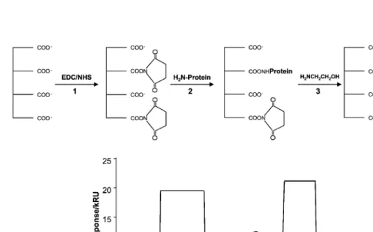
Ž .
Fig. 2. Example of a covalent immobilization of antibody on a CM5 sensor chip. 1 The carboxyl groups are reacted with a NHSrEDC
Ž . Ž
mixture and reactive NHS esters are formed. 2 The antibody solution is injected and coupling reaction through the primary amino groups
. Ž .
from the antibody lysine residues is allowed to proceed. 3 Remaining reactive NHS ester sites are blocked with ethanolamine
Ž . Ž .
5.1. Preconcentration assays
Fig. 1 illustrates the results of three sequential preconcentration assays. Using ca. 1700 RU as a reasonable immobilization level for the direct kinetic assay of small peptide binding to an antibody
sur-Ž
face, situation A 5 mgrml mAb in 10 mM acetate .
buffer, pH 5.5 is clearly the most satisfactory. In B Ž5 mgrml mAb in 10 mM formate buffer, pH 4.5 ,. mAb response increases rather slowly and the final
Ž mAb level is insufficient. In contrast, situation C 50
. mgrml mAb in 10 mM acetate buffer, pH 5.5 corresponds to a fast mAb uptake by the surface resulting in a too high mAb final density.
5.2. Antibody coÕalent immobilization
A standard ligand covalent immobilization moni-tored by SPR is depicted in Fig. 2. In a first stage
Ž .1 , the EDCrNHS activating mixture is injected with the consequent increase in the SPR signal due to a change in the bulk refractive index. The mAb Ž . solution is then injected and the binding event 2 can be followed in real time. Once the adequate binding level is reached, the remaining active car-boxyl-NHS esters are blocked with ethanolamine
Ž .
hydrochloride 3 , causing a significant change in the bulk refractive index. The biospecific mAb surface is
Ž . then ready to be used 4 .
5.3. Binding assays
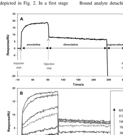
The binding assays consist of sequential peptide injection plus regeneration cycles. Fig. 3A shows the three main stages observed when monitoring the
Ž .
biospecific interaction in real time: 1 Analyte
bind-Ž . Ž .
ing to the immobilized ligand association . 2 Bound analyte detaching from the immobilized
lig-Ž . Ž . Ž .
Fig. 3. A One injection cycle. B Superposition of several binding curves sensorgrams corresponding to distinct injection cycles
Ž . Ž .
and dissociation in running buffer . 3 Ligand sur-face regeneration.
Each cycle corresponds to a new sample, so that all blanks, controls, different peptide concentrations
Ž and assay repeats are covered. When a full set i.e.,
.
all concentrations of a given peptide of injection
cycles is finished, the corresponding sensorgrams can be transformed in order to eliminate irrelevant
Ž .
regions e.g., regeneration pulses and to normalize the time and response axes. This results in the
super-Ž .
position of several sensorgrams Fig. 3B , ready to be processed by the curve fitting software.
Fig. 4. Illustration of the different stages in the analysis of the interaction between an FMDV peptide and an anti-FMDV neutralizing mAb.
ŽA Sensorgrams generated by injection of five distinct concentrations of a nonspecific peptide scrambled sequence on an anti-FMDV. Ž . Ž .
mAb surface. B Sensorgrams generated by injection of five distinct concentrations of a specific FMDV peptide on the same anti-FMDV
Ž . Ž .
mAb surface. C Corrected sensorgrams for the specific FMDV peptide-mAb interactions, obtained by subtraction of curves shown in A
Ž . Ž .
from the curves shown in B . D Residual data distribution for the association and dissociation phases, after global curve fitting to the 1:1
Ž . Ž .
bimolecular interaction model numerical integration . E Linear correlation between the analyte concentration, C, and the apparent rate
Ž . Ž .
constant, k , calculated by local curve fitting to the 1:1 bimolecular interaction model analytical integration . F Correlation between fitteds equilibrium response, R , and analyte concentration, C.eq
Table 1
Kinetic and affinity data from the SPR analysis of the peptide–immobilized antibody interaction illustrated in Fig. 4
y1 y1 y1 y1
w x Ž . Ž . Ž . Ž .
Curve fitting Peptide nM ka M s kd s KA M
4 y3 7 Global – 6.2 = 10 2.6 = 10 2.3 = 10 4 y3 7 Local, simultaneous k rka d 152 6.0 = 10 2.4 = 10 2.5 = 10 4 y3 7 305 5.8 = 10 2.6 = 10 2.3 = 10 4 y3 7 610 5.9 = 10 2.6 = 10 2.3 = 10 4 y3 7 1220 6.1 = 10 2.7 = 10 2.3 = 10 4 y3 7 2440 6.2 = 10 2.9 = 10 2.1 = 10 4 y3 7 Local, separate k rka d 152 6.7 = 10 2.4 = 10 2.8 = 10 4 y3 7 305 6.2 = 10 2.6 = 10 2.4 = 10 4 y3 7 610 5.5 = 10 2.6 = 10 2.1 = 10 4 y3 7 1220 5.8 = 10 2.8 = 10 2.1 = 10 4 y3 7 2440 5.9 = 10 2.7 = 10 2.2 = 10 7 w x Reqvs. peptide plot 2.0 = 10
Three different curve fitting methods were tested in order to evaluate the consistency of the fitted parameters.
5.4. Data processing and eÕaluation
Fig. 4 depicts the most important stages in data processing and evaluation. In A, sensorgrams corre-sponding to a nonspecific peptide injected on a mAb surface are shown. The sensorgrams are square-wave shaped due to a mere refractive index jump, which is confirmed by the fact that no peptide is bound to the mAb at the beginning of the dissociation phase. In B, sensorgrams correspond to a specific interaction be-tween an injected peptide and the immobilized mAb. This same interaction is depicted in C, after being corrected by subtraction of the sensorgrams
corre-Ž sponding to the nonspecific peptide analogue shown
.
in A . Sensorgrams in C were globally fitted to a 1:1 interaction model, with calculated curves totally co-incident with the experimental ones and residuals
Ž .
randomly distributed around zero Fig. 4D , corre-sponding to a chi-squared lower than 1. The kinetic parameters obtained are shown in Table 1. These sensorgrams were also fitted locally to the same
Ž .
kinetic model Table 1 .
Further local fitting was performed using the
sep-Ž .
arate k rka d model Table 1 and the locally fitted apparent rate constant, k , was plotted against pep-s
Ž .
tide to check the linearity k s k = C q ks a d
ex-Ž .
pected for a 1:1 interaction kinetics Fig. 4E . The locally fitted response at equilibrium, R , was alsoeq plotted against peptide concentration so that the
Ž .
affinity constant KA values withdrawn from this
plot and calculated by the k rka d ratio could be
Ž .
compared Table 1 .
6. Discussion 6.1. Trouble-shooting
6.1.1. Immobilization is not satisfactory
The immobilization level depends on several fac-tors, such as ligand concentration, pH, ionic strength,
Ž .
activation time EDCrNHS mixture and injection
Ž .
time ligand . Generally, lower ligand binding levels can be reached by decreasing ligand concentration, pH, activation and contact times or by increasing ionic strength. Conversely, higher concentrations and activation or contact times, as well as lower ionic strength, contribute to increase ligand immobilization levels.
6.1.2. Baseline responses increase oÕer repeated cycles
The regeneration step is not efficient and bound analyte is not fully washed off after each binding cycle. Regenerating agents must be tested and a
Ž .
cocktail approach Andersson et al., 1999a,b may be required.
6.1.3. Binding leÕels decrease oÕer repeated cycles
There is loss of ligand activity, either due to ligand inactivation under the analysis conditions
em-Ž . ployed inadequate buffers, regeneration agents, etc.
Ž
or to blockage of ligand binding sites extremely strong analyte-ligand interactions, ineffective
regen-.
eration steps . Different immobilization methodolo-gies or regeneration conditions may solve the prob-lem.
6.1.4. Expected binding is not obserÕed
If analyte or ligand degradation prior to usage in the biosensor experiments can be discarded, then ligand inactivation during immobilization must be suspected. Alternative immobilization strategies
Ž
should be tested e.g., thiol coupling, binding of biotinylated ligand to a streptavidin surface, immobi-lization of mAb to an anti-mouse Fc antibody
sur-. face .
6.1.5. Data do not fit to the expected kinetic model
Ž .
Generally, antigen–antibody Fab interactions display a Langmuirian behavior on the biosensor. Deviations from pseudo-first order kinetics, one of the most difficult problems to solve in biosensor
Ž
analysis Morton et al., 1995; O’Shannessy and Win-.
zor, 1996; Hall et al., 1996 , can arise from several factors. The consideration is that, when kinetic stud-ies are to be carried out, mass transport effects must be minimized. This can be achieved by decreasing
Ž
the ligand immobilization level e.g., to the mini-mum amount giving a satisfactory signal-to-noise
. Ž
ratio , or by increasing buffer flow rate always higher than 30 mlrmin and as high as sample
con-.
sumption, thus, permits , or by increasing analyte Ž
concentration as long as surface binding capacity is .
not saturated . Mass transport influence can be tested by analyzing the effect of different buffer flow rates
Ž
on analyte initial binding rates curve slopes at the .
initial stage of the association step . Another precau-tion aimed to eliminate mass transport effects in complex dissociation consists in using a ligand solu-tion instead of buffer during the dissociasolu-tion phase. Other common sources of deviation are ligand or analyte heterogeneity. The first is mainly due to random immobilization procedures and can be mini-mized by lowering binding levels or using oriented methodologies such as streptavidin–biotin or anti-Fc–Fc indirect immobilization. Analyte heterogene-ity can be reduced through additional sample purifi-cation steps.
The sources of deviation most difficult to deal with are those intrinsic to the binding partners or phenomena, such as analyte multivalency, avidity, or
Ž
complex binding mechanisms e.g., involving con-.
formational changes . When these effects are pre-sent, the only way to take them into account is to use the more complex fitting models included in the evaluation software, although it may be difficult to judge whether a good fit corresponds to the real
Ž .
binding mechanism Schuck, 1997 .
6.1.6. Buffer and sample refractiÕe indices mismatch
Whenever sample and running buffers are differ-Ž . ent, nonspecific bulk refractive index RI jumps
Ž
take place square-wave shaped signals superimpose .
to the binding curves . Although such bulk RI re-sponse may be eliminated by subtraction of a blank run, useful information from stages immediately af-ter the injection pulse may be lost. Thus, sample buffer should resemble the running buffer as close as possible.
6.1.7. Nonspecific binding
Nonspecific binding may become a problem when using unpurified samples, such as cell lysates, hy-bridomas, etc. Anyway, nonspecific binding should
Ž . be checked by one of the following ways. 1 Sample injection on both the specific cell and a reference cell. This reference cell must be prepared as
simi-Ž
larly as possible to the specific one e.g., same coupling chemistry to immobilize a similar amount
. Ž .
of inactivated ligand . 2 Another approach, perhaps more appropriate, consists of injection of a
non-Ž
specific analyte e.g., peptide with randomized se-.
quence .
BIAcore 2000 and 3000 instruments allow to monitor interactions on the four different sensor chip cells with a single sample injection, thus, providing simultaneous analysis of analyte binding to three different receptors plus a reference cell at minimal sample costs.
6.2. AlternatiÕe procedures
The direct single-step approach presented here is the simplest way to study biospecific interactions and is advisable for kinetic studies. However, some-times the systems under study cannot be suitably
characterized by this method and alternative ap-proaches may be required. Standard alternative SPR methodologies include the following:
6.2.1. Direct multistep approach
This consists of immobilization of a ligand fol-lowed by binding of a specific analyte folfol-lowed by
Ž
injection of a second binding partner that binds the .
first analyte is injected. Each binding stage is moni-tored in real-time and this approach is often
em-Ž .
ployed for binding site analysis Dubs et al., 1992 Ž
and analyte response enhancement Van Regenmor-.
tel et al., 1994 .
6.2.2. Indirect surface-competition assay
This is used in kinetic studies of low molecular weight analytes and consists of injecting a specific high molecular weight analyte followed by competi-tion experiments using the small target analyte as
Ž .
competitor Karlsson, 1994 . This requires a macro-molecule possessing the same binding specificity of
Ž
the small target analytes e.g., a viral protein compet-.
ing with a small peptide antigen .
6.2.3. Solution affinity experiments
These are widely employed for small analyte detection, with the disadvantage that they do not provide kinetic information. This approach resembles a competition ELISA experiment in the sense that a
Ž .
suitable analyte e.g., native peptide antigen is im-mobilized on the sensor surface and preincubated
Ž
mixtures of analyte–receptor e.g., other peptide .
antigens q specific antibody are injected. Incubating variable analyte concentrations with a constant re-ceptor concentration allows to build inhibition curves Ži.e., free receptor concentration vs. analyte
concen-.
tration , from which binding constants can be
with-Ž .
drawn Nieba et al., 1996; Gomes et al., 2001b,c,d .
7. Essential references 7.1. Original papers
v Fagerstam, L.G., Frostell-Karlsson, A., Karls-
¨
˚
Ž .
son, R., Persson, B. and Ronnberg, I. 1992
¨
v Hall, D.R., Cann, J.R. and Winzor, D.J. 1996Ž . v Karlsson, R. 1994Ž .
v Lofas, S. and Johnsson, B. 1990
¨
Ž .v Morton, T.A., Myszka, D. and Chaiken, I.
Ž1995.
v O’Shannessy, D.J. and Winzor, D.J. 1996Ž .
v O’Shannessy, D.J., Brigham-Burke, M. and
Ž .
Peck, K. 1992
v O’Shannessy, D.J., Brigham-Burke, M.,
Sone-Ž .
son, K.K., Hensley, P. and Brooks, I. 1993
7.2. ReÕiew papers
v Garland, P.B. 1996Ž . v Schuck, P. 1997Ž .
v Homola, J., Yee, S.S. and Gauglitz, G. 1999Ž .
7.3. Other sources
v ABiacore instrument handbook,B Biosensor
Ž1994.
v ABIAevaluation software handbook: version
Ž .
3.0,B Biosensor 1997
v ABIAplications handbook,B Biosensor 1994Ž .
v http:rrwww.biacore.com
8. Quick procedure
Ž .i Prepare peptide stock solutions, ca. 2.5 mM in 0.1 M acetic acid, and quantitate by amino acid analysis.
Ž .ii Prepare mAb stock solutions, ca. 15 mgrml in PBS, and quantitate by measuring optical density
w Ž
at 280 nm considering 1 OD280f0.75 mg pro-. x
tein rml .
Žiii Prepare mAb solutions for preconcentration. assays: start with four to six different solutions, at different pH and mAb concentrations. For instance,
v 5, 10 and 50 mgrml in 10 mM sodium maleate
buffer, pH 4.5;
v 5, 10 and 50 mgrml in 10 mM sodium acetate
buffer, pH 5.0;
v 5, 10 and 50 mgrml in 10 mM sodium acetate
buffer, pH 5.5.
Živ Prepare a 1-M ethanolamine hydrochloride. Ž
solution, adjusting the pH to 8.5 also available from .
Ž .v Set the biosensor instrument ready, according to the manufacturer’s instructions manual:
v replace the HBS running buffer available fromŽ
.
Biosensor bottle for a new one;
v dock a new sensor chip ŽBIAcertified CM5
.
sensor chip and prime the system;
v normalize the instrument signal, using the
BIAnormalizing solution.
Žvi Select one out the four flow cells on the. sensor chip and set the buffer flow rate to 5 mlrmin. Žvii Program an alternate series of 25-ml injec-. tions, corresponding to the different mAb solutions
Ž .
prepared in iii , and 5-ml injections of the 1 M Ž .
ethanolamine hydrochloride prepared in iv . Žviii Decide whether it is necessary to improve. preconcentration levels by adjusting mAb solution
Ž .
parameters concentration, pH, ionic strength . If Ž . Ž . improvement is required, repeat steps iii – vii . If not, choose the mAb solution giving the best results
Ž . Ž .
and follow steps ix and xx below, for covalent immobilization.
Žix Prepare 0.2 M EDC and 0.05 M NHS solu-. Ž
tions also available from Biosensor; these solutions, once prepared, should be divided into 100-ml aliquots
. and stored below 0 8C .
Ž .x Mix 50 ml of the EDC solution with an equal volume of the NHS solution, and immediately inject 35 ml of this mixture at 5 mlrmin, to activate the sensor surface. Solutions can be mixed using the automatic sampling unit of the instrument.
Žxi Inject 35 ml of the mAb solution chosen in. Žviii . Binding levels can be controlled at this stage. by either interrupting the injection or appending extra injections of the mAb solution.
Žxii Block the remaining active sites on the sur-. face with a 30-ml injection of 1 M ethanolamine hydrochloride, pH 8.5.
Žxiii. Prepare solutions for testing regeneration conditions, starting with the most commonly used for mAb–peptide binding assays:
v 10 mM HCl;
v 10 mM NaOH.
Žxiv Select a peptide expected to bind signifi-. Ž
cantly to the mAb e.g., the native antigenic
se-.
quence and dilute the stock solution to 600 nM in HBS.
Žxv Test the regenerating agents by alternating. injections of 15 ml of peptide and 10 ml of regenerat-ing solutions. If common regeneratregenerat-ing agents are not adequate, try other possibilities until an agent capa-ble of restoring the baseline level while keeping mAb binding activity is found. Then, proceed to the binding kinetics analyses as described below.
Žxvi Prepare a peptide dilution series: 1000-fold. and further serial dilutions of stock solution in HBS, covering six to eight different peptide concentrations Že.g., 2500–20 nM . Include the nonspecific peptide.
Ž .
dilution series and a blank sample HBS only . Žxvii. Replace the HBS bottle by a new one,
Ž . prime the system and normalize the signal as in v .
Žxviii Set the buffer flow rate to 60 mlrmin.. Žxix Program the injection cycle relevant opera-. Ž
. tional commands shown in italics :
v predip needle in HBS;
v kinject 90 ml of peptide solution plus 240 s
dissociation in running buffer;
v inject 60 ml of the regenerating solution; v extracleanup needle.
Each injection cycle corresponds to a single ana-lyte sample. Programmed cycles must cover all pep-tide concentrations plus nonspecific peppep-tide samples and blank runs. Flush the system whenever peptide is changed.
Žxx Prepare raw data obtained in xix for pro-. Ž . cessing with the BIAevaluation software: group in
Ž .
the same file all binding curves sensorgrams corre-Ž
sponding to the same peptide different concentra-.
tions , to the nonspecific peptide and to the blank runs.
Žxxi Following manufacturer’s instructions, nor-. malize all sensorgrams by setting all baseline levels
Ž .
to 0 RU response units and all injection starts to 0 s.
Žxxii Delete irrelevant parts of the sensorgrams,. such as the regeneration pulses, spikes and alike.
Žxxiii Transform the sensorgrams by subtracting. the blank run response.
Žxxiv Further correction of the experimental data. is done by subtraction of the nonspecific peptide
Ž .
spe-Ž
cific peptide binding curve for the same concentra-.
tion .
Žxxv Select the corrected peptide binding curves. and fit them globally to the simplest kinetic model Ž1:1 bimolecular interaction , choosing binding curve. regions as wide as possible so that injection pulses and bulk RI jumps are avoided.
Žxxvi Fit sensorgrams locally each binding curve. Ž .
separately to test for kinetic data consistency. Žxxvii Repeat sensorgram local fitting, now con-. sidering association and dissociation steps separately, as a further test for data consistency. Check for
Ž .
linearity of k s f Conc .s
Žxviii Judge on fitting model suitableness and. kinetic data reliability. If results are satisfactory, proceed to the next peptide. If not, other kinetic models can be tested or, most probably, the
experi-Ž
mental setup must be changed starting with mAb immobilization levels and peptide concentration
. range .
References
Altschuh, D., Dubs, M.C., Weiss, E., Zeder-Lutz, G., Van Regen-mortel, M.H.V., 1992. Determination of kinetic constants for the interaction between monoclonal antibody and peptides using surface plasmon resonance. Biochemistry 31, 6298– 6304.
Andersson, K., Areskoug, D., Hardenborg, E., 1999a. Exploring buffer space for molecular interactions. J. Mol. Recognit. 12, 36–43.
Andersson, K., Hamalainen, M., Malmqvist, M., 1999b. Identifi-cation and optimization of regeneration conditions for affinity-based biosensor assays. A multivariate cocktail ap-proach. Anal. Chem. 71, 2475–2481.
Brigham-Burke, M., Edwards, J.R., O’Shannessy, D.J., 1992. Detection of receptor–ligand interactions using surface plas-mon resonance: model studies employing the HIV-1 gp120r CD4 interaction. Anal. Biochem. 205, 125–131.
Chao, H., Houston, M.E., Grothe, S., Kay, C.M., O’Connor-Mc-Court, M., Irvin, R.T., Hodges, R.S., 1996. Kinetic study on the formation of a de noÕo designed heterodimeric coiled-coil: use of surface plasmon resonance to monitor the association and dissociation of polypeptide chains. Biochemistry 35, 12175–12185.
Cheskis, B., Freedman, L.P., 1996. Modulation of nuclear recep-tor interactions by ligands: kinetic analysis using surface plasmon resonance. Biochemistry 35, 3309–3318.
Dubs, M.C., Altschuh, D., Van Regenmortel, M.H.V., 1992. Mapping of viral epitopes with conformationally specific mon-oclonal antibodies using biosensor technology. J. Chromatogr. 597, 391–396.
England, P., Bregere, F., Bedouelle, H., 1997. Energetic and´ ` kinetic contributions of contact residues of antibody D1.3 in the interaction with lysozyme. Biochemistry 36, 164–172.
˚
Fagerstam, L., Frostell-Karlsson, A., Karlsson, R., Persson, B.,¨ Ronnberg, I., 1992. Biospecific interaction analysis using sur-¨ face plasmon resonance detection applied to kinetic, binding site and concentration analysis. J. Chromatogr. 597, 397–410. Gomes, P., Giralt, E., Andreu, D., 2000a. Surface plasmon reso-nance screening of synthetic peptides mimicking the immun-odominant region of C-S8c1 foot-and-mouth disease virus. Vaccine 18, 362–370.
Gomes, P., Giralt, E., Andreu, D., 2000b. Direct single-step surface plasmon resonance analysis of interactions between small peptides and immobilized monoclonal antibodies. J. Immunol. Methods 235, 101–111.
Gomes, P., Giralt, E., Andreu, D., 2001a. Molecular analysis of peptides from the GH loop of foot-and-mouth disease virus C-S30 using surface plasmon resonance: a role for kinetic rate constants. Mol. Immunol. 37, 975–985.
Gomes, P., Giralt, E., Andreu, D., 2001b. Antigenicity modulation upon peptide cyclization: application to the GH loop of foot-and-mouth disease virus strain C -Barcelona. Vaccine 9,1 3459–3466.
Gomes, P., Giralt, E., Andreu, D., 2001. Submitted for publica-tion.
Gomes, P., Giralt, E., Andreu, D., 2001. In preparation. Hall, D.R., Cann, J.R., Winzor, D.J., 1996. Demonstration of an
upper limit to the range of association rate constants amenable to study by biosensor technology based on surface plasmon resonance. Anal. Biochem. 235, 175–184.
Homola, J., Yee, S.S., Gauglitz, G., 1999. Surface plasmon resonance sensors: review. Sens. Actuators, B 54, 3–15. Houshmand, H., Froman, G., Magnusson, G., 1999. Use of bacte-¨
riophage T7 displayed peptides for determination of mono-clonal antibody specificity and biosensor analysis of the bind-ing reaction. Anal. Biochem. 240, 209–214.
Huyer, G., Li, Z.M., Adam, M., Huckle, W.R., Ramachandran, C., 1995. Direct determination of the sequence recognition requirements of the SH2 domains of SH-PTP2. Biochemistry 34, 1040–1049.
Karlsson, R., 1994. Real-time competitive kinetic analysis of interactions between low-molecular-weight ligands in solution and surface-immobilized receptors. Anal. Biochem. 221, 142– 151.
Lasonder, E., Bloemhoff, W., Welling, G.W., 1994. Interaction of lysozyme with synthetic anti-lysozyme D1.3 antibody frag-ments studied by affinity chromatography and surface plasmon resonance. J. Chromatogr., A 676, 91–98.
Lasonder, E., Schellekens, G.A., Koedjik, D.G.A.M., Damhof, R.A., Welling-Wester, S., Fejilbrrief, M., Scheffer, A.J., Welling, G.W., 1996. Kinetic analysis of synthetic analogues of linear-epitope peptides of glycoprotein D of herpes simplex virus type I by surface plasmon resonance. Eur. J. Biochem. 240, 209–214.
Lemmon, M.A., Ladbury, J.E., Mandiyan, V., Zhou, M., Sch-lessinger, J., 1994. Independent binding of peptide ligands to the SH2 and SH3 domains of Grb2. J. Biol. Chem. 269, 31653–31658.
Lessard, I.A.D., Fuller, C., Perhm, R.N., 1996. Competitive inter-action of component enzymes with the peripheral subunit-bi-nding domain of the pyruvate–dehydrogenase multienzyme complex of Baccilus stearothermophilus: kinetic analysis us-ing surface plasmon resonance detection. Biochemistry 35, 16863–16870.
Lookene, A., Chevreuil, O., Østergaard, P., Olivecrona, G., 1996. Interaction of lipoprotein lipase with heparin fragments and with heparan sulfate: stoichiometry, stabilization and kinetics. Biochemistry 35, 12155–12163.
Malmqvist, M., Karlsson, R., 1997. Biomolecular interaction anal-ysis: affinity biosensor technologies for functional analysis of proteins. Curr. Opin. Chem. Biol. 1, 378–383.
Morton, T., Myszka, D., Chaiken, I., 1995. Interpreting complex binding kinetics from optical biosensors: a comparison of analysis by linearization, the integrated rate equation and numerical integration. Anal. Biochem. 227, 176–185. Nieba, L., Krebber, A., Plukthun, A., 1996. Competition BIAcore¨
for measuring true affinities: large differences from values determined from binding kinetics. Anal. Biochem. 234, 155– 165.
Oddie, G.W., Gruen, L.C., Odgers, G.A., King, L.G., Kortt, A.A., 1997. Identification and minimization of nonideal binding effects in BIAcore analysis: ferritinranti-ferritin Fab’ interac-tion as a model system. Anal. Biochem. 253, 103–111. O’Shannessy, D.J., Winzor, D.J., 1996. Interpretation of
devia-tions from pseudo-first order kinetic behavior in the characteri-zation of ligand binding by biosensor technology. Anal. Biochem. 236, 275–283.
O’Shannessy, D.J., Brigham-Burke, M., Soneson, K.K., Hensley, P., Brooks, I., 1993. Determination of rate and equilibrium binding constants for macromolecular interactions using sur-face plasmon resonance: use of nonlinear least squares meth-ods. Anal. Biochem. 212, 457–468.
Richalet-Secordel, P.M., Rauffer-Bruyere, N., Christensen, L.L.,´ Ofenloch-Haehnle, B., Seidel, C., Van Regenmortel, M.H.V., 1997. Concentration measurement of unpurified proteins using biosensor technology under conditions of partial mass trans-port limitation. Anal. Biochem. 249, 165–173.
Saunal, H., Van Regenmortel, M.H.V., 1995. Mapping of viral conformational epitopes using biosensor measurements. J. Im-munol. Methods 183, 33–41.
Schuck, P., 1997. Use of surface plasmon resonance to probe the equilibrium and dynamic aspects of interactions between bio-logical macromolecules. Annu. Rev. Biophys. Biomol. Struct. 26, 541–566.
Schuck, P., Minton, A.P., 1996. Kinetic analysis of biosensor data: elementary tests for auto-consistency. Trends Rev. Biochem. Sci. 21, 458–460.
Shen, B.J., Hage, T., Sebald, W., 1996. Global and local determi-nants for the kinetics of interleukin-4rinterleukin-4 receptor a chain interaction: a biosensor study employing recombinant interleukin-4 binding protein. Eur. J. Biochem. 240, 252–261. Tamamura, H., Otaka, A., Murakami, T., Ishihara, T., Ibuka, T., Waki, M., Matsumoto, A., Yamamoto, N., Fujii, N., 1996. Interaction of an anti-HIV peptide, T22, with gp120 and CD4. Biochem. Biophys. Res. Commun. 219, 555–559.
Van Regenmortel, M.H.V., Altschuh, D., Pellequer, J.L., Richalet-Secordel, P., Saunal, H., Wiley, J.A., Zeder-Lutz, G., 1994.´ Analysis of viral antigens using biosensor technology. Meth-ods: Comp. Methods Enzymol. 6, 177–197.
VanCott, T.C., Bethcke, F.R., Polonis, V.R., Gorny, M.K., Zolla-Pazner, S., Redfield, R.R., Birx, D.L., 1994. Dissociation rate of antibody-gp120 binding interactions is predictive of V3-mediated neutralization of HIV-1. J. Immunol. 153, 449–458. Wu, Z., Johnsson, K., Choi, Y., Ciardelli, T.L., 1995. Ligand binding analysis of soluble interleukin 2-receptor complexes by surface plasmon resonance. J. Biol. Chem. 270, 16045– 16051.
Zeder-Lutz, G., Rauffer, N., Altschuh, D., Van Regenmortel, M.H.V., 1995. Analysis of cyclosporin interactions with anti-bodies and cyclophilin using BIAcore. J. Immunol. Methods 183, 131–140.
Zeder-Lutz, G., Zuber, E., Witz, J., Van Regenmortel, M.H.V., 1997. Thermodynamic analysis of antigen-antibody binding using biosensor measurements at different temperatures. Anal. Biochem. 246, 123–132.