Performance of Photon Reconstruction and Identification with the CMS Detector in Proton-Proton Collisions at sqrt(s) = 8 TeV

EUROPEAN ORGANIZATION FOR NUCLEAR RESEARCH (CERN)

CERN-PH-EP/2013-037 2015/08/24

CMS-EGM-14-001

Performance of photon reconstruction and identification

with the CMS detector in proton-proton collisions at

_√

s

=

8 TeV

The CMS Collaboration

Abstract

A description is provided of the performance of the CMS detector for photon recon-struction and identification in proton-proton collisions at a centre-of-mass energy of 8 TeV at the CERN LHC. Details are given on the reconstruction of photons from en-ergy deposits in the electromagnetic calorimeter (ECAL) and the extraction of photon energy estimates. The reconstruction of electron tracks from photons that convert to electrons in the CMS tracker is also described, as is the optimization of the photon energy reconstruction and its accurate modelling in simulation, in the analysis of the Higgs boson decay into two photons. In the barrel section of the ECAL, an energy resolution of about 1% is achieved for unconverted or late-converting photons from H→γγdecays. Different photon identification methods are discussed and their cor-responding selection efficiencies in data are compared with those found in simulated events.

Published in the Journal of Instrumentation as doi:10.1088/1748-0221/10/08/P08010.

c

2015 CERN for the benefit of the CMS Collaboration. CC-BY-3.0 license

∗_{See Appendix A for the list of collaboration members}

1

1

Introduction

This paper describes the reconstruction and identification of photons with the CMS detector [1] in data taken in proton-proton collisions at √s = 8 TeV during the 2012 CERN LHC running period. Particular emphasis is put on the use of photons in the observation and measurement of the diphoton decay of the Higgs boson [2]. For this decay mode, the energy resolution has significant impact on the sensitivity of the search and on the precision of measurements made in the analysis. The uncertainties related to the photon energy scale are the dominant contri-butions to the systematic uncertainty in the Higgs boson mass, mH = 124.70±0.31 (stat)±

0.15 (syst) GeV, measured in Ref. [2]. The procedure employed to optimize the photon energy estimation and its accurate modelling in the simulation is described. This procedure relies on the large sample of recorded Z boson decays to dielectrons, whose showers are reconstructed as photons, and on simulation to model differences in detector response to electrons and photons. The reconstruction of photons from the measured energy deposits in the electromagnetic cal-orimeter (ECAL) [3] and the extraction of a photon energy estimate is described, as well as the association of the electron tracks to clusters in the ECAL for photons that convert in the tracker. A large fraction of the energy deposited in the detector by all proton-proton interactions arises from photons originating in the decay of neutral mesons, and these electromagnetic showers provide a substantial background to signal photons. The use and interest of photons as signals or signatures in measurements and searches is therefore mainly focussed on those with high transverse momentum where this background is less severe. Photon selection methods used for the H →γγchannel and other analyses are described, together with measurements of the selection efficiency. The efficiency measured in data is compared with that found in simulated events.

The paper starts with brief descriptions of the CMS detector (Section 2), paying particular at-tention to geometrical details of the electromagnetic calorimeter that are important for shower reconstruction, and of the data and simulated event samples used (Section 3). Section 4 de-scribes photon reconstruction in CMS: clustering of the shower energy deposited in the ECAL crystals, correction of the cluster energy and fine tuning of the calibration, photon energy res-olution, and uncertainties in the photon energy scale. Section 5 describes the reconstruction of the electron tracks resulting from photons that undergo conversion before reaching the ECAL. Section 6 discusses the separation of prompt photons from energy deposits originating from the decay of neutral mesons, describing two identification algorithms, and giving results on their performance. The main results are summarized in Section 7.

2

CMS detector

The central feature of the CMS apparatus is a superconducting solenoid of 6 m internal di-ameter, providing a magnetic field of 3.8 T. Within the superconducting solenoid volume are a silicon pixel and strip tracker, a lead tungstate crystal electromagnetic calorimeter, and a brass/scintillator hadron calorimeter (HCAL), each one composed of a barrel and two endcap sections. Muons are measured in gas-ionization detectors embedded in the steel flux-return yoke outside the solenoid. Extensive forward calorimetry complements the coverage provided by the barrel and endcap detectors. A more detailed description of the CMS detector can be found in Ref. [1].

The pseudorapidity coordinates, η, of detector elements are measured with respect to the coor-dinate system origin at the centre of the detector, whereas the pseudorapidity of reconstructed particles and jets is measured with respect to the interaction vertex from which they originate.

The transverse energy, denoted by ET, is defined as the product of energy and sin θ, with θ

being measured with respect to the origin of the coordinate system.

Charged-particle trajectories are measured by the silicon pixel and strip tracker, with full az-imuthal coverage within |η| < 2.5. Consisting of 1 440 silicon pixel detector modules and 15 148 silicon strip detector modules, totalling about 10 million silicon strips and 60 million pixels, the silicon tracker provides an impact parameter resolution of≈15 µm and a transverse momentum, pT, resolution of about 1.5% for charged particles with pT=100 GeV [4].

The total amount of material between the interaction point and the ECAL, in terms of radiation lengths ( X0), raises from 0.4 X0 close to η = 0 to almost 2 X0 near|η| = 1.4, before falling to about 1.3 X0around|η| =2.5. The probability of photon conversion before reaching the ECAL is thus large and, since the resulting electrons (e+e−pairs) emit bremsstrahlung in the material, the electromagnetic shower of some photons starts to develop in the tracker. The electrons are deflected by the 3.8 T magnetic field, resulting in multiple electromagnetic showers in the ECAL.

The ECAL is a homogeneous and hermetic calorimeter made of lead tungstate, PbWO4,

scin-tillating crystals. The high density (8.28 g cm−3_{), short radiation length (8.9 mm), and small}

Moli`ere radius (23 mm) of the PbWO4 crystals enabled the construction of a compact

calori-meter with fine lateral granularity. The central barrel covers |η| < 1.48 with the inner sur-face located at a radius of 1290 mm. The endcaps cover 1.48 < |η| < 3.00 and are located at

|z| > 3154 mm. A preshower detector consisting of two planes of silicon sensors interleaved with a total of 3 X0of lead is located in front of the endcaps and covers 1.65< |η| <2.60. The ECAL barrel is made of 61 200 trapezoidal crystals with front face transverse sections of about 22×22 mm2_{, giving a granularity of 0.0174 in η and φ. The crystals have a length of}

230 mm (25.8 X0). Each half-barrel is formed by 18 barrel supermodules each covering 20◦ in

φand containing 85×20 = 1700 crystals. The crystals of a half-barrel may be viewed as po-sitioned in a regular rectangular grid in(η, φ)space (which wraps round on itself in φ), and indexed by 85×360 integer pairs. The supermodules are composed of four modules. Within the modules there are submodules each containing two rows of five crystals. The void between adjacent crystals within the same submodule is 350 µm wide. The void between adjacent crys-tals in adjacent submodules is 550 µm wide. The voids between adjacent cryscrys-tals separated by module and supermodule boundaries are about 6 mm wide. The module boundaries occur at

|η| = 0, 0.435, 0.783, and 1.131, and the supermodules boundaries occur every 20◦ in φ. The geometry is quasi-projective, with almost all the crystal axes tilted by an angle of 3◦ with re-spect to the line from the coordinate origin in both the η and φ directions, and only the void at η= 0 points to the origin—the 3◦ tilt relative to the η direction is introduced progressively for the first five rings of crystals away from this boundary.

The ECAL endcaps are made of 14 648 trapezoidal crystals (7324 each) with a front face trans-verse section of 28.6×28.6 mm2_{, and a length of 220 mm (24.7 X}

0). The crystals are grouped

in 5×5 crystal structural units, with the crystals in adjacent units being separated by a void of 2 mm. The voids between adjacent crystals within the 5×5 units are 350 µm wide. Each endcap is constructed as two half-disks. The crystals are installed within a quasi-projective geometry pointing 1300 mm beyond the centre of the detector, giving tilts of 2◦to 8◦relative to the direction of the coordinate origin.

3

3

Data and simulated event samples

The results presented here use data corresponding to an integrated luminosity of 19.7 fb−1 taken at a centre-of-mass energy of 8 TeV.

The Monte Carlo (MC) simulation of the response of the CMS detector employs a detailed de-scription of it, and uses GEANT4 version 9.4 (patch 03) [5]. The simulated events include the presence of multiple pp interactions taking place in each bunch crossing weighted to repro-duce the distribution of the number of such interactions in data. The presence of signals from multiple pp interactions in each recorded event is known as pileup. Interactions taking place in a preceding or a following bunch crossing, i.e. within a window of±50 ns around the trigger-ing bunch crosstrigger-ing, are included. The interactions used to simulate pileup are generated with PYTHIA6.426 [6], the same version that is used for other purposes as described below.

Samples of simulated Higgs boson events produced in gluon-gluon and vector-boson fusion processes are obtained using the next-to-leading-order matrix-element generatorPOWHEG (ver-sion 1.0) [7–11] interfaced withPYTHIA. For the associated Higgs boson production with W and Z bosons, and with tt pairs,PYTHIAis used alone.

Direct-photon production in γ+jet processes is simulated usingPYTHIAalone. Nonresonant diphoton processes involving two prompt photons are simulated usingSHERPA1.4.2 [12]. The SHERPA samples are found to give a good description of diphoton continuum events accom-panied by one or two jets. To complete the description of the diphoton background in the H → γγ channel, the remaining processes where one of the photon candidates arises from misidentified jet fragments are simulated withPYTHIA. The cross sections for these processes are scaled to match their values measured in data, using the K-factors at 8 TeV that were ob-tained at 7 TeV [13, 14].

Simulated samples of Z→e+_e−_{and Z→}

µ+µ−γevents, generated with MADGRAPH5.1 [15], SHERPA, and POWHEG [16], are used for some tests, for comparison with data, and for the derivation of energy scale corrections in data and resolution corrections in the simulations. The simulation of the ECAL response has been tuned to match test beam results, and uses a detailed simulation of the 40 MHz digitization based on an accurate model of the signal pulse as a function of time. The effects of electronics noise, fluctuations due to the number of pho-toelectrons, and the amplification process of the photodetectors are included. The simulation also includes a spread of the single-channel response corresponding to the estimated intercali-bration precision, an additional 0.3% constant term to account for longitudinal nonuniformity of light collection, and the few nonresponding channels identified in data. The measured in-tercalibration uncertainties range from 0.35% in most of the barrel, to 0.9% at the end of the fourth barrel module, and 1.6% in most of the region covered by the endcaps with a steep rise for|η| >2.3.

As a general rule, for the simulation of data taken at 7 and 8 TeV, the response variation with time is not simulated. However, for the simulation of photon signals and Z-boson background samples used for data-MC comparisons of the photon energy scale, energy resolution, and pho-ton selection, two refinements are implemented: the changes in the energy-equivalent noise in the electromagnetic calorimeter during the data-taking period are simulated, and a signifi-cantly increased time window (starting 300 ns before the triggering bunch crossing) is used to simulate out-of-time pileup. These refinements improve the agreement between data and sim-ulated events, seen when comparing distributions of shower shape variables, and they provide improved corrections to the energy measurement.

4

Photon reconstruction

Photons for use as signals or signatures in measurements and searches, rather than for use in the construction of jets or missing transverse energy, are reconstructed from energy deposits in the ECAL using algorithms that constrain the clusters to the size and shape expected for electrons and photons with pT & 15 GeV. The algorithms do not use any hypothesis as to

whether the particle originating from the interaction point is a photon or an electron, conse-quently electrons from Z→e+e−events, for which pure samples with a well defined invariant mass can be selected, can provide excellent measurements of the photon trigger, reconstruction, and identification efficiencies, and of the photon energy scale and resolution. The reconstructed showers are generally limited to a fiducial region excluding the last two crystals at each end of the barrel (|η| <1.4442). The outer circumferences of the endcaps are obscured by services passing between the barrel and the endcaps, and this area is removed from the fiducial region by excluding the first ring of trigger towers of the endcaps (|η| > 1.566). The fiducial region terminates at|η| =2.5 where the tracker coverage ends.

The photon reconstruction proceeds through several steps. Sections 4.1, 4.2, and 4.3 cover the intercalibration of the individual channels, the clustering of recorded energy signals resulting from showers in the calorimeter, and the energy assignment to a cluster. Section 4.4 discusses the procedure used in the H →γγanalysis to (i) obtain corrections for fine-tuning the photon energy assignment in data, and (ii) tune the resolution of simulated photons reconstructed in MC samples. Section 4.5 examines the resulting photon resolution in data and in simulation. Section 4.6 discusses the estimation of the uncertainty in the energy scale after implementing the corrections obtained in Section 4.4.

4.1 Calibration of individual ECAL channels

The calorimeter signals in data must be calibrated and corrected for several detector effects [17]. The crystal transparency is continuously monitored during data taking by measuring the re-sponse to light from a laser system, and the observed changes are corrected for when the events are reconstructed. The relative calibration of the individual channels is achieved using the φ-symmetry of the energy deposited by pileup and the underlying event, the invariant mass measured in two photon decays of π0 and η mesons, and the momentum measured by the tracker for isolated electrons from W and Z boson decays.

4.2 Clustering

Clustering of ECAL shower energy is performed on intercalibrated, reconstructed signal am-plitudes. The clustering algorithms collect the energy from radiating electrons and converted photons that gets spread in the φ direction by the magnetic field. These algorithms are de-scribed in detail in Ref. [18], and evolved from fixed matrices of 5×5 crystals, which provide the best reconstruction of unconverted photons, by allowing extension of the energy collection in the φ direction, to form “superclusters”. Clusters are built starting from a “seed crystal”: one containing a signal corresponding to a transverse energy greater than those of all its immediate neighbours and above a predefined threshold. In the barrel, where the crystals are arranged in an(η, φ)grid, the clusters have a fixed width of five crystals centred on the seed crystal, in the η direction. In the φ direction, adjacent strips of five crystals are added if their summed energy is above another predefined threshold. Further clusters, aligned in η, may be seeded and added to the original, “seed”, cluster if they lie within an extended φ window (seed crystal

±17 crystals)—under the control of a further predefined threshold. Clustering in the endcaps uses fixed matrices of 5×5 crystals. After a seed cluster has been defined, further 5×5

matri-4.3 Correction of cluster energy 5

ces are added if their centroid lies within a small η window and within a φ distance roughly equivalent to the 17 crystals span used in the barrel. The 5×5 matrices are allowed to partially overlap one another. For unconverted photons, the superclusters resulting from both the barrel and endcap algorithms are usually simply 5×5 matrices.

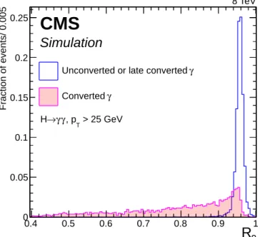
The R9variable is defined as the energy sum of the 3×3 crystals centred on the most energetic

crystal in the supercluster divided by the energy of the supercluster. The showers of photons that convert before reaching the calorimeter have wider transverse profiles and lower values of R9 than those of unconverted photons. Figure 1 shows the R9 distribution for photons in

the ECAL barrel that convert in the material of the tracker before a radius of 85 cm, and those that convert later, or do not convert at all before reaching the ECAL. The events are simulated Higgs boson diphoton decays, H → γγ, and the photons are required to satisfy pT > 25 GeV.

Both histograms are normalized to unity. Despite being an imperfect indicator of whether a photon converts before reaching the ECAL, R9 is strongly correlated with the photon energy

resolution degradation due to the spreading of showers initiated in the tracker, induced by the magnetic field. Based on such information, the simplest energy estimation for photons is made by summing the energy in the supercluster for barrel (endcap) photons with R9 < 0.94

(R9 <0.95), and summing the energy in a 5×5 crystal matrix for the remaining “unconverted”

photons. Signals recorded in the preshower detector are included in the region|η| >1.65.

9

R

Unconverted or late converted

γ Converted > 25 GeV T , p γ γ → H 8 TeV

CMS

Simulation

Figure 1: Distributions of the R9 variable for photons in the ECAL barrel that convert in the

material of the tracker before a radius of 85 cm (solid filled histogram), and those that convert later, or do not convert at all before reaching the ECAL (outlined histogram).

4.3 Correction of cluster energy

Significant improvements in energy resolution are obtained by correcting the initial sum of en-ergy deposits forming the supercluster for the variation of shower containment in the clustered crystals and for the shower losses of photons that convert before reaching the calorimeter. The main mechanisms resulting in systematic variation of the fraction of the initial energy con-tained in the clustered crystals, ranked in approximate order of increasing severity, are

(i) variation of longitudinal depth at which the shower passes through the off-pointing in-tercrystal voids (causing variation of longitudinal containment),

(ii) variation of shower location with respect to the lateral granularity (causing variation of lateral containment),

(iii) variation in the amount of energy absorbed before reaching the ECAL for showers start-ing before the ECAL,

(iv) variation in the extent to which the energy of showers starting before the ECAL is clus-tered, and,

(v) if the shower passes through an intermodule void, the variation of longitudinal depth at which the shower passes through it.

The direction of a shower crossing any of the voids between adjacent crystals (detailed in Sec-tion 2) makes an angle of about 3◦ relative to the crystal sides. The result is a loss of crystal depth seen by the shower. For a 350 µm void the loss of depth is small: 0.35 mm/ sin 3◦ ≈

6.7 mm (about 0.75 X0). For the 6 mm intermodule voids the loss of depth is equal to about half

a crystal length. The effect of such a reduction of calorimeter thickness depends on the shower development at the depth at which the void is crossed.

Corrections as a function of η, ET, R9, and the lateral extension of the cluster in φ, have been

obtained from the observed losses in simulated events, and used in many data analyses [19– 24]. Corrections have also been extracted from data, using photons from final state radiation in dimuon decays of Z bosons [19], although limits on precision start to be severe for pT>30 GeV

since the steeply falling pTspectrum of these photons limits the number available.

To obtain the best possible energy resolution for the H → γγ analysis [2] the energy mea-surement is obtained using a multivariate regression technique. The H → γγ analysis uses events containing pairs of photons with an invariant mass in the range 100< mγγ <180 GeV, with the threshold on the lowest pT photon set at mγγ/4. This corresponds to pT > 25 GeV for all photons used in the analysis, and pT & 30 GeV for photons used in the estimation of

the mass of the Higgs boson at 125 GeV. The photon energy response is parameterized by a function with a Gaussian core and two power law tails, an extended form of the Crystal Ball function [25]. The regression provides an estimate of the parameters of the function for a single photon, and consequently a prediction of the probability distribution of the ratio of true energy to uncorrected energy. The corrected photon energy is taken from the most probable value of this distribution. The input variables are the η coordinate of the supercluster, the φ coordinate of barrel superclusters, and a collection of shower shape variables: R9of the supercluster, the

energy weighted η-width and φ-width of the supercluster, and the ratio of the energy in the HCAL behind the supercluster and the energy of the supercluster. In the endcap, the ratio of preshower energy to raw supercluster energy is also included.

Additional information is included for the seed cluster of the supercluster: the relative energy and position of the seed cluster, the local covariance matrix of the magnitude of the crystal energy signals, and a number of energy ratios of crystal matrices of different sizes defined with respect to the position of the seed crystal. These variables provide information on the likelihood and location of a photon conversion and the degree of showering in the material between the interaction vertex and the calorimeter, and together with their correlation with the η and φ position of the supercluster, drive the magnitude of containment correction predicted by the regression. In the barrel, the η and φ indices of the seed crystal, as well as the position of the

4.3 Correction of cluster energy 7

seed cluster with respect to the seed crystal are also included. These variables, together with the seed cluster energy ratios, provide information on the amount of energy that is likely to be contained in the cluster, or lost in the intermodule voids, and drive the corrections for local containment predicted by the regression. Although the variations of local containment and the losses due to showering that starts in the tracker material are different effects, the corrections are allowed to be correlated in the regression to account for the fact that a showering photon is not incident on the ECAL at a single point, and is consequently less affected by variations of local containment.

Finally, the number of primary vertices and the median transverse energy density ρ [26] in the event are included in order to allow for the correction of residual systematic effects due to the average amount of pileup in the event.

The semiparametric regression is trained to predict the true energy of the photon, Etrue, given

the uncorrected supercluster energy. The uncorrected energy, Eraw, is taken as the sum of

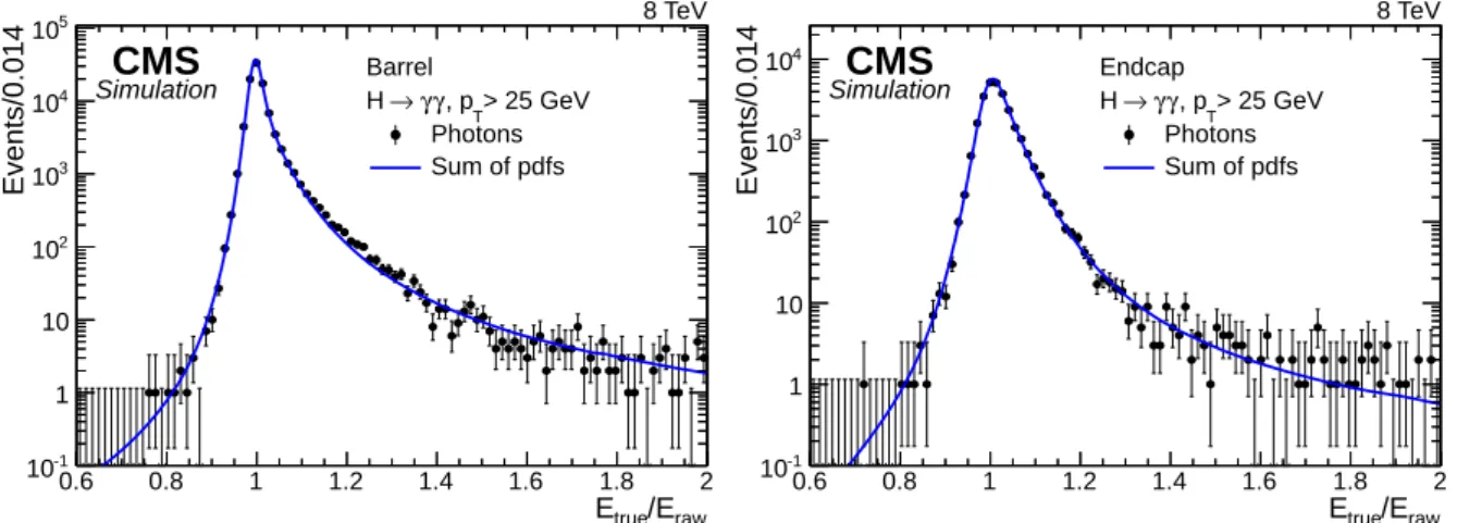
indi-vidual crystal energies in a supercluster. After training, the regression predicts the full proba-bility density function (pdf) for the inverse response, Etrue/Eraw, for each individual photon. In

Fig. 2 the sum of predicted distributions for photons with pT > 25 GeV in simulated H → γγ events is compared to the observed distribution of Etrue/Eraw. The agreement is excellent,

al-though there are deviations, e.g. in the barrel at Etrue/Eraw ≈ 1.2, that are larger than can be

explained by the statistical uncertainties, and although at Etrue/Eraw ≈ 1.2 the probability is

down by more than two orders of magnitude from the peak the deviation points to the exis-tence of systematic effects in the event-by-event estimate of the tails of the energy response. The prediction of the pdf for the inverse response is used in the H → γγanalysis to estimate the mass resolution of individual diphoton systems, which assists in the classification of diphoton events, and is shown here for information. The energy of photon superclusters is taken to be the most probable value of the pdf, and the performance of this specific assignment, which is probed by the assessment of the resolution in Section 4.5, is therefore independent of the details of the pdf. raw /E true E 0.6 0.8 1 1.2 1.4 1.6 1.8 2 Events/0.014 -1 10 1 10 2 10 3 10 4 10 5 10 8 TeV

CMS

Simulation Barrel _{> 25 GeV}

T , p γ γ → H Photons Sum of pdfs raw /E true E 0.6 0.8 1 1.2 1.4 1.6 1.8 2 Events/0.014 -1 10 1 10 2 10 3 10 4 10 8 TeV

CMS

Simulation Endcap _{> 25 GeV}

T , p γ γ → H Photons Sum of pdfs

Figure 2: Comparison of the distribution of the inverse response, Etrue/Eraw, in simulated

events (points with error bars) with the sum of the pdfs predicted by the regression (curve). The comparison is made using a set of simulated photons independent of the training sample, in the (left) ECAL barrel and (right) endcap.

4.4 Fine tuning of calibration and simulated resolution

In the H→ γγanalysis the final calibration of the energy measurement in data and the mod-elling of the energy resolution in simulation were fine-tuned. Electron showers from rather pure samples (the background contribution is<0.1%) of Z bosons decaying to electrons were reconstructed as photons, using only the information in the ECAL and without using any in-formation from the tracker. The dielectron invariant mass was then calculated using the vertex position obtained from the electron tracks, and its distribution compared to that obtained in simulated events.

The corrections required are small. They comprise a correction to the energy scale for the data, and a correction to the energy resolution of the MC simulation (achieved by adding a Gaussian distributed random contribution to the energy reconstructed in simulated events). Before the fine-tuning the data have already been corrected for variations of crystal transparency, and the individual crystals have been intercalibrated. The simulation of the showers in the ECAL includes these uncertainties. The increase of the energy-equivalent noise during the data-taking period is also simulated. The noise variation is due to a gradual increase of the leakage current in the silicon avalanche photodiodes used in the ECAL barrel region, and due to response loss in the endcap, with the amount of variation depending on η.

Three explanations have been suggested for the need of an additional smearing of the energy estimate in simulated events to achieve complete agreement with the data. The slightly worse energy resolution may be explained by

(i) the presence of more tracker material in the detector, between the interaction point and the ECAL, than in the simulation,

(ii) underestimation of the uncertainty in the individual crystal calibration—although it would be difficult to reconcile a significant underestimation with the fact that the individual crystal calibration uncertainties have been obtained by detailed comparisons among dif-ferent methods of intercalibration,

(iii) residual differences between the actual ECAL geometry and the one implemented in the simulation so that the energy correction estimates, obtained by multivariate regression from simulated events, are suboptimal for data.

Measurements (discussed in Section 4.6) show that there is, indeed, more tracker material present in the detector than is simulated, and this results in worse energy resolution for pho-tons that convert in the tracker, and an increase in their number. This fact, however, does not account for all the observed resolution discrepancies, which include the need to worsen the simulated resolution of showers for which the R9variable has a high value (corresponding to

photons that convert late or not at all). The other two factors listed above represent further contributions in addition to that from mismodelling of tracker material, although their rela-tive magnitude is not known [17]. While additional intercalibration errors would increase the constant term in the fractional energy resolution, the contributions of the other effects have an energy dependence. As described below, the applied smearing is allowed to have an energy-dependent component.

The supercluster energy scale is tuned and corrected by varying the scale in the data to match that observed in simulated events. Two procedures have been used to obtain these corrections: the “fit method” and the “smearing method”. The fit method uses an analytic fit to the Z boson invariant mass peak, with a convolution of a Breit–Wigner distribution with a Crystal

4.4 Fine tuning of calibration and simulated resolution 9

Ball function. Distributions obtained from data and from simulated events are fitted separately and the results are compared to extract a scale offset. The Breit–Wigner width is fixed to that of the Z boson: ΓZ = 2.495 GeV [27]. The parameters of the Crystal Ball function, which gives

a reasonable description of the calorimeter resolution effects and of bremsstrahlung losses in front of the calorimeter, are left free in the fit. The smearing method uses the simulated Z-boson invariant mass shape as a probability density function in a maximum likelihood fit. All the known detector effects, reconstruction inefficiencies, and the Z-boson kinematics are taken into account in the simulation. The residual discrepancy between data and simulation is described by an energy smearing function. A Gaussian smearing applied to the simulated response has been found to be adequate to describe the data in all the categories of events examined. A larger number of electron shower categories can be handled by the smearing method as compared to the fit method.

The procedure implemented to fine-tune the energy scale has three steps for the barrel, and two steps for the endcap calorimeters. In each step, the parameters defining the scale and the width are both allowed to float in the fit, and corrections to the scale are extracted. Only in the final step, the third step for the barrel and the second step for the endcaps, are energy smearing corrections extracted for application to simulated events.

The first step corrects for possible time dependencies during data taking by extracting, with the fit method, the scale correction to be applied to the data for each data-taking epoch (51 epochs defined by ranges of run numbers), and for each region in absolute pseudorapidity (4 bins, two in the barrel and two in the endcaps). This step was originally introduced to account for possible imperfections in the transparency corrections. However the transparency corrections obtained from the laser monitoring system during 8 TeV data taking are of quality such that there is very little variation to correct. This can be seen from Fig. 3, which shows the ratio of the energy measured by the ECAL over the momentum measured by the tracker, E/p, for electrons selected from W→ eν decays, as a function of the date at which they were recorded. The magnitudes of the energy scale corrections extracted in the first step of the fine-tuning procedure are thus small, generally<0.1% in the barrel and<0.2% in the endcaps.

The second step derives corrections for effects mainly related to the material in front of the calorimeter, and uses the smearing method. Showers are classified in two R9bins in each of two

barrel and two endcap pseudorapidity regions, yielding eight shower categories. Combining different pairs of shower categories, 36 Z→e+e−invariant mass distributions are constructed for both data and simulated events. The shower energies in simulated events are modified by applying a Gaussian multiplicative random factor with a mean value 1+∆P and a standard

deviation ∆σ. The method maximizes the likelihood of the fit between the invariant mass distributions as a function of the 16 parameters (∆P and ∆σ for each shower category), for the full Z→e+e−data sample, including events where the two showers are in different categories. The energy scale discrepancies found in this step are shown in Table 1 together with their uncertainties. The corrections that must be applied to the data are the reciprocals of these values.

The large Z → e+e−data sample provides sufficient statistical precision for the third step to be performed in the barrel. This step introduces ET-dependent corrections to the energy scale

using 20 bins defined by ranges in|η|, R9, and ET using the smearing method as in the second

step. In this step the smearing procedure is iterated because the value of the corrections applied can change the ETbin into which a photon falls. Convergence is achieved after three iterations.

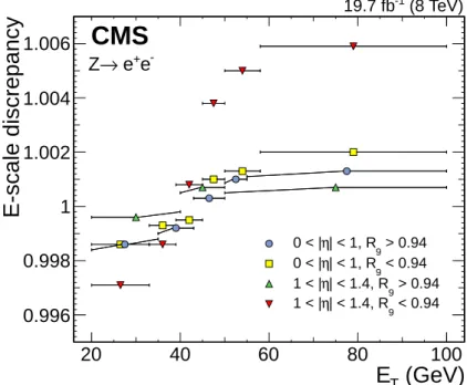
The residual discrepancies measured in this final step are shown, as a function of ET, in Fig. 4,

date (day/month)

19/04 19/05 18/06 18/07 17/08 16/09 16/10 15/11

Relative E/p scale

0.93 0.94 0.95 0.96 0.97 0.98 0.99 1 1.01 1.02

without laser monitoring correction with laser monitoring correction

CMS ECAL barrel (8 TeV) -1 19.7 fb 0 100 200 Mean 1 RMS 0.0009 Mean 0.95 RMS 0.011 date (day/month) 19/04 19/05 18/06 18/07 17/08 16/09 16/10 15/11

Relative E/p scale

0.7 0.75 0.8 0.85 0.9 0.95 1 1.05 1.1

without laser monitoring correction with laser monitoring correction

CMS ECAL endcap (8 TeV) -1 19.7 fb 0 50 100 150 Mean 1 RMS 0.0028 Mean 0.82 RMS 0.037

Figure 3: Ratio of the energy measured by the ECAL over the momentum measured by the tracker, E/p, for electrons selected from W → eν decays, as a function of the date at which they were recorded. The ratio is shown both before (red points), and after (green points), the application of transparency corrections obtained from the laser monitoring system, and for both the barrel (upper plot) and the endcaps (lower plot). Histograms of the values of the measured points, together with their mean and RMS values are shown beside the main plots.

Table 1: Energy scale discrepancies, and associated statistical uncertainties, found in the second step of the fine-tuning procedure. The corrections that must be applied to the data are the reciprocals of these values.

Category Scale deviation Uncertainty

|η| <1, R9 ≥0.94 1.0021 0.42×10-4 R9 <0.94 0.9993 0.33×10-4 1< |η| <1.44, R9 ≥0.94 1.0097 2.06×10-4 R9 <0.94 0.9987 0.63×10-4 1.57< |η| <2, R9 ≥0.94 1.0058 2.27×10-4 R9 <0.94 0.9989 1.05×10-4 2< |η| <2.5, R9 ≥0.94 1.0023 1.26×10-4 R9 <0.94 0.9973 1.52×10-4

4.4 Fine tuning of calibration and simulated resolution 11

used for photons with ET >100 GeV. It can be seen from the figure that the largest corrections

obtained in the third and final step are for photons with R9 <0.94 and|η| >1.

The energy scale corrections finally applied to the data are the product of the corrections ex-tracted in the steps described above. The smearing to be applied to the simulated energy res-olution, extracted in the second step for the endcaps and in the third step for the barrel, is modelled by an amplitude and a mixing angle specifying the sharing of this amplitude be-tween a constant term and a 1/√E term, providing thereby an extra degree of freedom to the energy resolution uncertainty. The uncertainties and correlations from the fit contribute to the systematic uncertainty in the energy resolution. In the endcaps, it is not possible to determine the sharing between a constant and energy dependent term, and therefore the smearing is taken to be constant, not varying with energy. The corrections to the resolution of the simulated pho-tons range from≈0.7 (1)% to 1 (2)% in the barrel for high (low) R9, respectively, and from 1.6

to 2.0% in the endcaps. In the barrel, the uncertainties in these values are about 10% of the values themselves. In the endcaps the uncertainties are about 15% for the two most relevant photon categories, and up to 50% for the categories which contribute few event to the H→γγ analysis. The uncertainties are assessed by (i) examining the variation of the R9distribution as

a function of η and comparing it to what is observed for photons, (ii) changing the R9 value

used for categorization, (iii) using an energy estimate for the electron showers based on an electron-trained regression rather than the photon regression, (iv) changing the pTthreshold of

the sample used, and (v) changing the identification criteria used to select the electrons. The effect of these systematic uncertainties on the Higgs boson mass determination is <10 MeV, and they have little impact (<1%) on the significance of the signal.

(GeV)

E

E-scale discrepancy

CMS

Figure 4: Residual discrepancies in the photon energy scale obtained for the barrel in the final step of the fine-tuning procedure, as a function of ET, for different η and R9 categories. The

statistical uncertainties in these values are negligible. The horizontal error bars indicate the ranges of the ET bins. The reciprocals of these values are applied as corrections to the energy

4.5 Photon energy resolution

Figure 5 shows the electron pair invariant mass reconstructed in Z→e+e−events in the 8 TeV data and simulated events where the electrons are reconstructed as photons, and the full set of photon corrections and smearings is applied. The resulting distributions are shown separately for the case where both showers are in the barrel, and for the case where at least one of the showers is in an endcap. The distributions of simulated events are normalized to match the distributions in data. In the panels beneath the main plots, the ratio of the number of events in data to the number of simulated events in each bin is shown, together with a band obtained by propagating the uncertainties in the simulated energy resolution, and the energy scale in data, to the dielectron masses obtained. There is excellent agreement between the simulation and data in the cores of the distributions. A slight discrepancy is present in the low-mass tail in the endcaps, where the Gaussian smearing cannot account for some noticeable non-Gaussian effects. Since the electron showers are reconstructed as photons, the mass peaks do not appear at the true Z-boson mass, both in data and in the simulation. This is because the fraction of the original particle energy contained in a supercluster is, on average, a little smaller for electrons than for photons, and consequently the photon energy regression imperfectly estimates the energy of electron showers. With respect to the uncorrected distributions, the corrections to the data shift the peak by about−0.5 GeV for the case where both the showers are in the barrel, and by about−1 GeV if either of the showers is in an endcap. In addition, the distributions obtained from data are slightly narrower after the corrections. The distributions for the simulated events after the correction procedure are wider, because of the applied smearing.

Events/0.5 GeV 0 2 4 6 8 10 12 14 16 18 20 After correction Data (MC) -e + e → Z 4 10 ×

CMS

CMS

Figure 5: Reconstructed invariant mass distribution of electron pairs in Z → e+e− events in data (points) and in simulation (histogram). The electrons are reconstructed as photons and the full set of photon corrections and smearings are applied. The comparison is shown for (left) events with both showers in the barrel and (right) the remaining events. For each bin, the ratio of the number of events in data to the number of simulated events is shown in the panels beneath the main plot. The band shows the systematic uncertainty in the ratio originating in the systematic uncertainty in the simulated energy resolution, and in the data energy scale.

4.5 Photon energy resolution 13

The single-photon energy resolution in Z → e+e− events where the electron showers are re-constructed as photons has been measured in both data and simulated events using a method similar to, but independent of, that used to obtain the corrections and smearings. The data and simulated event samples are the same as those used to obtain the corrections and smearings. The fitting methodology allows the resolution and energy scale for single showers to be ex-tracted in fine bins of chosen variables, but with the limitation that the energy resolution for each bin is parameterized as a Gaussian distribution. Figure 6 shows the resolution measured in small bins of η, taken as the position of the shower in the ECAL, for showers with R9 ≥0.94

and R9 < 0.94, for data and simulated events. The vertical dashed lines show the barrel

mod-ule boundaries, where the resolution is somewhat degraded, and the grey band at |η| ≈ 1.5 marks the barrel-endcap transition region excluded from the photon fiducial region used in the H → γγ analysis. The simulated resolution matches the resolution observed in data as a function of η very well. There is a small systematic difference in the endcap, particularly for the photons with R9 <0.94, with the simulated photons showing worse energy resolution than

the photons in data. This is understood as being a result of the methodology used to determine the resolution, which focuses on the Gaussian core of the distribution. In this region, the Gaus-sian smearing added to the simulation in the fine-tuning step is larger than elsewhere, and the smearing truly required here would have a non-Gaussian tail.

Figure 6 demonstrates the very good agreement between simulation and data achieved for the resolution of electron showers reconstructed as photons. This is an important achievement, but it does not provide a measurement of the energy resolution of photons. Electron showers tend to have worse energy resolution than photon showers of the same energy since all elec-trons radiate to some extent in the material of the tracker, even those with high values of R9.

Furthermore, the fitting technique used to obtain the resolution shown in Fig. 6, parameterizes the resolution as a Gaussian distribution and thus tends to be more sensitive to the core of the resolution function and less sensitive to its non-Gaussian tail. Additionally, it is of particu-lar interest to examine the energy resolution achieved for photons resulting from the decay of Higgs bosons, which are on average more energetic than the electrons resulting from the decay of Z bosons.

Since there is excellent agreement between data and simulation for electron showers, the energy resolution of photons in simulated events provides an accurate estimate of their resolution in data. Figure 7 shows the distribution of reconstructed energy divided by the true energy, Emeas/Etrue, of photons in simulated H→γγevents that pass the selection requirements given in Ref. [2], in a narrow η range in the barrel, 0.2< |η| <0.3. The distribution for photons with R9 ≥ 0.94 is shown on the left, and that for photons with R9 < 0.94 is shown on the right.

The width of the distribution is parameterized in two ways: by the half-width of the narrowest interval containing 68.3% of the distribution, σeff, and by the full-width-at-half-maximum of the

distribution divided by 2.35, σHM. These parameters are both equal to the standard deviation in

the case of a purely Gaussian distribution. Since σHMmeasures the width of the Gaussian core

of the distribution, the values are smaller, particularly where non-Gaussian tails make a larger contribution: for example, for R9<0.94 and at the intermodule boundaries. Figure 8 shows the

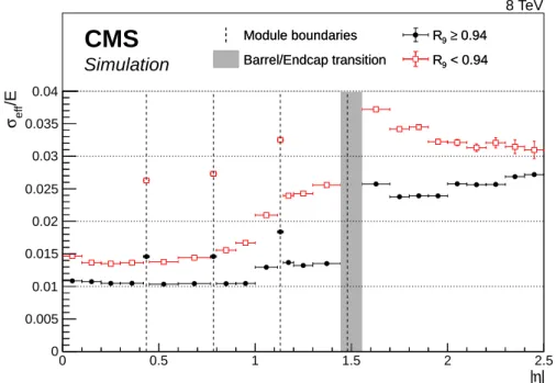
fractional energy resolution, parameterized as σ_eff/E, as a function of η, in simulated H→ γγ events that pass the analysis selection requirements. A bin size of 0.1 in η has been used, with adjustments to allow a small bin of width 0.03 centred on the barrel module boundaries where it can be seen that the resolution is locally degraded.

| η Supercluster | 0 0.5 1 1.5 2 2.5 / E σ 0 0.01 0.02 0.03 0.04 0.05 0.06 (8 TeV) -1 19.7 fb CMS (8 TeV) -1 19.7 fb CMS 0.94 ≥ 9 MC , R 0.94 ≥ 9 Data, R | η Supercluster | 0 0.5 1 1.5 2 2.5 / E σ 0 0.01 0.02 0.03 0.04 0.05 0.06 (8 TeV) -1 19.7 fb CMS (8 TeV) -1 19.7 fb CMS < 0.94 9 MC , R < 0.94 9 Data, R

Figure 6: Relative photon energy resolution measured in small bins of absolute supercluster pseudorapidity in Z → e+e−events, for data (solid black circles) and simulated events (open squares), where the electrons are reconstructed as photons. The resolution is shown for (upper plot) showers with R9 ≥ 0.94 and (lower plot) R9 < 0.94. The vertical dashed lines mark the

module boundaries in the barrel, and the vertical grey band indicates the range of|η|, around the barrel/endcap transition, removed from the fiducial region.

4.5 Photon energy resolution 15 true /E meas E 0.8 0.85 0.9 0.95 1 1.05 1.1 Events/0.0025 0 500 1000 1500 2000 2500 3000 3500 4000 4500 | < 0.3 η | ≤ 0.2 0.94 ≥ 9 R = 0.010 eff σ = 0.009 HM σ 8 TeV CMS Simulation | < 0.3 η | ≤ 0.2 0.94 ≥ 9 R = 0.010 eff σ = 0.009 HM σ (MC) γ γ → H true /E meas E 0.8 0.85 0.9 0.95 1 1.05 1.1 Events/0.0025 0 200 400 600 800 1000 1200 1400 1600 | < 0.3 η | ≤ 0.2 < 0.94 9 R = 0.013 eff σ = 0.011 HM σ 8 TeV CMS Simulation | < 0.3 η | ≤ 0.2 < 0.94 9 R = 0.013 eff σ = 0.011 HM σ (MC) γ γ → H

Figure 7: Distribution of measured over true energy, Emeas/Etrue, for photons in simulated

H → γγ events, in a narrow η range in the barrel, 0.2 < |η| < 0.3, (left) for photons with R9≥0.94, and (right) R9<0.94. | η | 0 0.5 1 1.5 2 2.5 /E e ff σ 0 0.005 0.01 0.015 0.02 0.025 0.03 0.035 0.04 Module boundaries R9≥ 0.94 Barrel/Endcap transition R9 < 0.94 Module boundaries R9≥ 0.94 Barrel/Endcap transition R9 < 0.94 8 TeV

CMS

Figure 8: Relative energy resolution, σeff/E, as a function of|η|, in simulated H→ γγ events, for photons with R9≥0.94 (solid circles) and photons with R9<0.94 (open squares). The

verti-cal dashed lines mark the module boundaries in the barrel, and the vertiverti-cal grey band indicates the range of|η|, around the barrel/endcap transition, removed from the fiducial region.

4.6 Energy scale uncertainty

The photon energy scale has been checked with photons in Z→ µ+µ−γevents. After a selec-tion of events ensuring a pure and unbiased sample of photons, there is agreement between the measured photon energy and that predicted from the known Z-boson mass and measured muon momenta. The overall energy scale difference between data and simulation found with the Z→µ+µ−γevents (using the fine-tuning corrections, obtained as described in Section 4.4) is 0.25%±0.11% (stat)±0.17% (syst). The study is made for photons with pT >20 GeV, and the

mean pTof the photons selected is 28 GeV. When binned in pT(so as to probe possible

nonlin-earities), and in R9and η (according to the known dependencies of the ECAL), the agreement

of the measurements with the defined energy scale remains good, although the uncertainties in individual bins are, at best, between 0.2 and 0.3%. Thus this check does not provide a very strong constraint on the uncertainty in the Higgs boson mass arising from the uncertainty in the photon energy scale. An additional limitation is that the check is for a range of photon energies that has only a limited overlap with that used in the Higgs boson analysis. For these reasons the uncertainty in the Higgs boson mass arising from the uncertainty in the photon energy scale has been analysed as described below.

There are three main sources of systematic uncertainty in the energy scale that is defined by the fine-tuning described in Section 4.4. These uncertainties are the main contributions to the systematic uncertainty in the measured mass of the Higgs boson in the diphoton decay chan-nel [2]. The largest uncertainties are due to the possible imperfect simulation of (i) differences in detector response to electrons and photons, and (ii) energy scale nonlinearity. Finally there is an uncertainty resulting from the procedure and methodology described in Section 4.4. These uncertainties are discussed in detail in Ref. [2] and summarized below together with additional results and information.

Since the energy scale has been obtained using electron showers reconstructed as photons, an important source of uncertainty in the photon energy scale is the imperfect modelling of the difference between electrons and photons by the simulation. The most important cause of the imperfect modelling is an inexact description of the material between the interaction point and the ECAL. Figure 9 shows the thickness of the tracker material in terms of radiation lengths, as inferred from data, relative to what is inferred from simulated events, as a function of|η|. The two methods used to infer the material thickness employ the energy loss of electrons in Z →

e+e−events and the energy loss of low transverse momentum, 0.9 < pT < 1.1 GeV,

charged-hadron tracks, where the momentum loss is computed from the change in the track curvature between the beginning and end of the track. The measurement using low-pT charged hadrons

is difficult to implement in the regions of the tracker at large η, and no values are available beyond|η| =2, but for|η| <1.6 the two methods give results that are in good agreement. In addition, there is no charged-hadron measurement for the bin centred at|η| =0.95 where the transition between the tracker barrel and endcap results in few tracks with the number of hits required to make a good measurement.

The difference between data and simulation in the material thickness of the tracker is almost certainly due to mismodelling of specific structures and localized regions. This hypothesis is supported by studies of the location of low-pT (down to pT ≈ 1 GeV) photon conversion

ver-tices, as shown in Ref. [28]. The results shown in Fig. 9, however, assume a simple scaling of the overall thickness. The effect of changes in the amount of tracker material on the relative dif-ference between the electron and photon energy scales has been studied with events simulated using tracker models where the amount of material is increased uniformly by 10, 20, and 30%. Mismodelling of localized structures may affect the measurements used to infer thickness in

4.6 Energy scale uncertainty 17 | η | 0 0.5 1 1.5 2 2.5 MC / X data X 0.9 1 1.1 1.2 1.3 1.4 1.5 Electron track Hadron track (8 TeV) -1 19.7 fb

CMS

Figure 9: Tracker material thickness (in terms of radiation lengths) inferred in the data, Xdata,

relative to that inferred in simulated events, XMC, as a function of |η|, using electrons in Z →

e+e−events (circles), and low-momentum charged hadrons (squares).

Fig. 9 somewhat differently from the way it affects the relative difference between the electron and photon energies. Therefore it is necessary to be rather conservative in the assignment of a systematic uncertainty. It is assumed that the effects on the energy scale are covered by a 10% uniform deficit of simulated material in the region|η| < 1.0 and a 20% uniform deficit for|η| >1.0. The resulting uncertainty in the photon energy scale has been assessed using the simulated samples in which the tracker material is increased uniformly, and ranges from 0.03% in the central ECAL barrel up to 0.3% in the outer endcap.

Since the longitudinal profiles of energy deposition of electrons and photons differ, a further difference in response between electrons and photons which would result from imperfect simu-lation, is related to modelling of the varying fraction of scintillation light reaching the photode-tector as a function of the longitudinal depth in the crystal at which it was emitted. Ensuring adequate uniformity of light collection was a major accomplishment in the development of the crystal calorimeter and was achieved by depolishing one face of each barrel crystal. However, an uncertainty in the achieved degree of uniformity remains and, in addition, the uniformity is modified by the radiation-induced loss of transparency of the crystals. The uncertainty re-sults in a difference in the energy scales between electrons and unconverted photons that is not present in the standard simulation. The effect of the uncertainty, including the effect of radiation-induced transparency loss, has been studied.

A scaling as a function of depth, measured from the front face of the crystal, is applied to the deposited energy. In the standard simulation this scaling is uniformly equal to unity, i.e. flat, for all except the rearmost 10 cm of the crystal. To simulate nonuniformity of light collection, an appropriate slope is introduced based on laboratory light-collection efficiency measurements made on the crystals, and measurements of its dependence on crystal transparency. The slope of the light collection efficiency as a function of depth, at the time when the ECAL was con-structed, is taken to be−0.14±0.08%/X0[29, 30], for the front half of the crystal (“front

coef-ficient induced by irradiation measured in m−1,∆µ, and is given by ∆F= 0.4%×∆µ/X₀[31]. Finally, the induced absorption coefficient is related to the light-yield (LY) loss measured by the laser monitoring system,∆(LY/LY0), through∆µ = k×∆(LY/LY0), where k =0.02%/m (i.e.

taking the average value of the measurements reported in Refs. [32] and [33]).

The uncertainty in the slope is taken as the difference between the flat response used in the standard simulation and the average slope measured at the time of ECAL construction plus the slope change resulting from the maximum radiation-induced light loss in the barrel. The resulting magnitude of the uncertainty in the photon energy scale in the barrel is 0.04% for pho-tons with R9 > 0.94 and 0.06% for those with R9 < 0.94, but the signs of the energy shifts are

opposite since unconverted photons penetrate deeper into the crystal than electrons, whereas converted photons share their energy between two electrons, whose showers thus penetrate the crystal less than a single electron shower. In the endcaps, the magnitude of the uncertainty in the photon energy scale is taken to be the same as in the barrel, and the effect of the longi-tudinal uniformity has not been studied in detail, firstly because the uncertainty in the energy scale due to other effects is larger there, and secondly because these studies were done in the context of the H →γγ analysis where uncertainties in the endcap energy scale had very little impact on the overall mass scale uncertainty. For the diphoton mass in the H → γγ analysis the two anticorrelated uncertainties result in an uncertainty of about 0.015% in the mass scale. The effect of the tracker material uncertainty on this value, where a changed tracker material budget would change the number of photons that convert in the tracker material, is negligible. In assessing the systematic uncertainties for the H → γγmass measurement, differences be-tween MC simulation and data in the extrapolation from shower energies typical of electrons from Z → e+e− decays to those typical of photons from H → γγ decays, were also investi-gated. The linearity of the energy response was studied in two ways: by examining the depen-dence of the energy-momentum ratio, E/p, of isolated electrons from Z and W boson decays as a function of ET, and by looking at the invariant mass of dielectrons from Z boson decays as

a function of the scalar sum of the transverse energies of the two electron showers, HT. In both

cases, the energy or transverse energy of the electrons and the invariant mass of the dielectron, are those obtained when the ECAL showers are reconstructed as photons. The showers are required to satisfy ET > 25 GeV and the photon identification requirements of the H → γγ analysis (with the electron veto removed). The E/p distributions, obtained from simulated events for a number of bins in ET, and the dielectron invariant mass distributions, obtained for

a number of bins in HT, were fitted to the corresponding distributions obtained from events

in data. A scale factor was extracted from each fit, whose difference from unity measures the residual discrepancy of the energy response in data relative to that in simulated events. As a cross-check, an iterated truncated-mean method was used to estimate the E/p or dielectron invariant mass peak positions and gave consistent results.

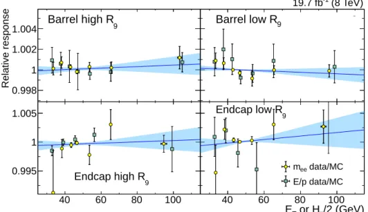
The results are shown in Fig. 10 for both the E/p and the dielectron invariant mass analyses. The points coming from the analysis of the dielectron mass are plotted as a function of HT/2.

The four panels show results for different η and R9 categories, with the dielectron analysis

restricted to events where both electron showers fall in the same category. The η categories correspond to the barrel and endcap regions. The horizontal error bars indicate the uncertainty in the mean ET or HT/2 for the bin, but for most bins that uncertainty is negligible and hidden

behind the plotted central value marker. In the endcaps for low R9the point corresponding to

ET = 95.4 GeV for the E/p analysis has a value of 1.0146 which does not fit in the plot scale,

although the lower vertical error bar, extending down below 1, can be seen. The differential nonlinearity is estimated from a linear fit through the points (shown by the lines). The uncer-tainties in the fit parameters of a linear response model, shown by the bands, are extracted after

4.6 Energy scale uncertainty 19

scaling the uncertainties such that the χ2per degree of freedom of the fits is equal to unity. The stability of the result has been checked by removing the points of the dielectron mass analysis that have very small statistical uncertainties (i.e. where HT/2 is about half the Z-boson mass).

40 60 80 100 Relative response 0.998 1 1.002 1.004 Barrel high R9 40 60 80 100 CMS (8 TeV) -1 19.7 fb 9 Barrel low R 40 60 80 100 0.995 1 1.005 9 Endcap high R /2 (GeV) T or H T E 40 60 80 100 9 Endcap low R data/MC ee m E/p data/MC

Figure 10: Residual discrepancy of the energy response in data relative to that in simulated events as a function of transverse energy (for the E/p analysis, squares) and of HT/2 (for the

di-electron mass analysis, circles) in four η and R9categories. The dielectron analysis is restricted

to events where both the electron showers fall in the same η, R9category. The uncertainties in

the fit parameters of a linear response model are shown by bands—further details are given in the text.

A value of 0.1% was assigned to the uncertainty in the effect of differential nonlinearity for a diphoton mass around 125 GeV in all events except those in the class in which the diphoton transverse momentum is particularly high, so that the highest transverse momentum photon in the event typically has pT >100 GeV. For this event class the uncertainty is set at 0.2%.

The digitization of the ECAL signals uses 12-bit analogue-to-digital-converters (ADCs) and, to increase the dynamic range, three different preamplifiers with different gains are used for each crystal, each with its own ADC, and the largest unsaturated digitization is recorded together with two bits coding the ADC number [1]. The possibility that imperfect matching between the different “gain ranges” introduces an uncertainty in the energy of the measured photons was investigated. The effect of switching preamplifiers for digitizing large signals, E & 200 GeV in the barrel and ET & 80 GeV in the endcaps, was found to be negligible for photons from

Higgs boson decays. The fraction of photons for which the lower-gain preamplifiers are used is small (<2%) and the lower-gain preamplifiers appear to be very well calibrated to the high-gain preamplifiers.

A further small uncertainty arises from imperfect electromagnetic shower simulation. A sim-ulation made with a shower description using the Seltzer–Berger model for the bremsstrahlung energy spectrum [34], which represents an improvement over GEANT4 version 9.4.p03, changes the energy scale for both electrons and photons. The much smaller changes in the difference between the electron and photon energy scales, although mostly consistent with zero, are in-terpreted as a limitation on our knowledge of the correct simulation of the showers, leading to a further uncertainty of 0.05% in the mass of the Higgs boson.

The statistical uncertainties in the measurements used to set the energy scale are small, but the methodology, which is described in Section 4.4, has a number of systematic uncertainties related to the imperfect agreement between data and MC simulation. The uncertainties range from 0.05% for unconverted photons in the ECAL central barrel to 0.1% for converted photons in the ECAL outer endcaps.

Accounting for all the contributions, the uncertainty in the photon energy scale at pT ≈mZ/2,

where mZis the Z boson mass, is about 0.1% in the central barrel, 0.15% in the outer barrel, and

0.3% in the endcaps. These uncertainties are largely correlated. The exact values, their correla-tions in two R9times four η bins, together with the contribution from the residual nonlinearity

and from the uncertainties on the energy and mass resolution have been propagated to the signal model of the H→γγanalysis. Together with similar, and not entirely correlated, uncer-tainties in the 7 TeV data they contribute 0.14 GeV to the systematic uncertainty of 0.15 GeV in the Higgs boson mass measurement [2].

5

Conversion track reconstruction

Photons traversing the CMS tracker have a sizeable probability of converting into electron-positron pairs. Although converted photons are fully clustered in the ECAL as described in Section 4, and identified with good approximation by the R9shower-shape variable, additional

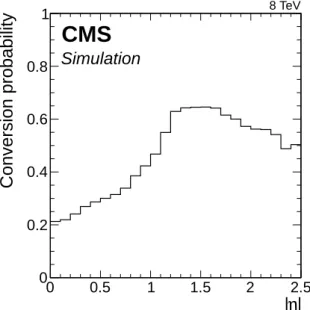
useful information is gained by reconstructing the associated e+e− track pairs. According to simulation, the fraction of photon conversions occurring before the last three layers of the tracker (reconstruction of conversion tracks requires at least three layers) is as high as about 60% in the pseudorapidity regions with the largest amount of tracker material in front of the ECAL (Fig. 11). Fully reconstructed conversions are used in the particle-flow reconstruction algorithm [35, 36]: the association of electron-track pairs with energy deposits in the ECAL avoids their being misidentified as charged hadrons, thus improving the determination of the photon isolation, as discussed in Section 6. The direction of the electron-track pair is also ex-ploited in assisting the determination of the longitudinal coordinate of the interaction vertex in the H→γγanalysis [2]. The aim of this section is to describe the methods used to reconstruct electron-track pairs and show the level of agreement between data and simulation in a very pure sample of photons.

Conversion reconstruction uses the full CMS tracking power [4]. Track reconstruction is based on an iterative tracking procedure. The first iteration aims at finding tracks originating from the interaction vertex while subsequent iterations aim at finding tracks from displaced (sec-ondary) vertices at increasing distance from the primary vertex. In addition, tracks starting from clusters in the ECAL and propagated inward into the tracker volume are sought, so as to reconstruct late-occurring conversions [37]. All tracks associated to the main electron recon-struction [18], as well as the subsample of the standard tracks which can be associated to energy deposits in the ECAL, are possible electron candidates and are refitted with the Gaussian sum filter method [38]. Tracks reconstructed as electrons are selected with basic quality require-ments on the minimum number of hits and goodness of the track fit. Tracks are then required to have a positive charged-signed transverse impact parameter (the primary vertex lies out-side the trajectory helix). Track-pairs of opposite charge are then filtered to remove tracks that might have resulted from conversions in the beam pipe, or could possibly consist of electrons originating from the primary vertex. Additional requirements on the track pair are meant to specifically identify the photon conversion topology. Photon conversion candidates can be dis-tinguished from massive meson decays, nuclear interactions or vertices from misreconstructed tracks by exploiting the fact that the momenta of the conversion electrons are approximately

21 | η | 0 0.5 1 1.5 2 2.5 Conversion probability 0 0.2 0.4 0.6 0.8 1 8 TeV

CMS

Figure 11: Fraction of photons converting before the last three layers of the tracker as func-tion of absolute pseudorapidity as measured in a simulated sample of H → γγ events. The conversion location is obtained from the simulation program.

parallel since the photon is massless. For this purpose, the angular separation of the track pair in the longitudinal plane, measured in terms of ∆ cot θ, is required to be less than 0.1. Also, the two-dimensional distance of minimum approach between the two tracks is required to be positive to remove intersecting helices. Finally, the point in which the two tracks are tangent is required to be well contained in the tracker volume.

Track pairs surviving the selection are fitted to a common vertex with a 3D-constrained kine-matic vertex fit. The 3D constraint imposes the tracks to be parallel in both transverse and longitudinal planes. The pair is retained if the vertex fit converges and the χ2 probability is greater than a given threshold. The transverse momentum of the pair is finally refitted with the vertex constraint.

Reconstructed conversions are required to satisfy a minimum transverse momentum threshold, meant to reduce accidental or poorly reconstructed pairs. The threshold on the converted pho-ton pTas measured by the tracks can vary depending on the application: in this paper, mainly

focussing on medium to high transverse momentum, the threshold is chosen to be 10 GeV. More than one conversion track-pair candidate can be reconstructed for the same superclus-ter. When such a case occurs, the optimal conversion is chosen by finding the best directional match between the momentum direction of the track pair and the position of the supercluster. The matching criterion is expressed in terms of the∆R=

√

∆η2_+∆φ2_{distance between the}

su-percluster direction and the conversion direction. The conversion candidate with minimum∆R is retained if∆R is less than 0.1. Both the conversion and supercluster directions are redefined with respect to the fitted conversion vertex position.

A sample of Z →µ+µ−γevents with a photon resulting from final-state radiation (FSR) is se-lected from dimuon-triggered data, together with a corresponding sample of simulated events. A very high photon purity (98%) is achieved in the selection, which is not reachable in any other sample. Events from Z → µ+µ−γ decays are selected by requiring the presence of two high-quality muon tracks reconstructed with both the muon detector and the tracker within

track is also required to be associated to small energy deposits in the hadron calorimeter. The dimuon invariant mass is required to be above 35 GeV.

Photon candidates are selected with loose identification criteria and with transverse momen-tum above 10 GeV, within|η| <2.5 (excluding the ECAL barrel-endcap transition region) and added to the dimuon system. The distance of the photon from the closest muon is required to satisfy∆R< 0.8, while the muon furthest from the photon must satisfy pT > 20 GeV. It is

re-quired that the track of the muon closest to the photon is not reconstructed also as an electron. Finally the three-body invariant mass, mµµγ, is required to satisfy 60< mµµγ<120 GeV. Figure 12 shows the µµγ invariant mass for events in which a conversion track pair, matched to the photon, has also been reconstructed. The invariant mass is calculated using the photon energy measured in the ECAL and taking the dimuon vertex. The distributions are normalized to the number of candidates in data and show good agreement between data and simulation.

Events / 1 GeV 0 500 1000 Data Simulation

Simulation: statistical uncertainty

γ µ µ → Z (8 TeV) -1 19.7 fb

CMS

(GeV)

m

Figure 12: Invariant mass for Z → µ+µ−γevents in which the photon is associated to a con-version track pair in data (points with error bars) and simulation (filled histogram).

An estimator of the quality of the conversion reconstruction is the matching between the en-ergy measured in the ECAL and the momentum measured from the track pair after refitting with the conversion vertex constraint. If the track pair is correctly reconstructed and associated to the right cluster in the calorimeter the ratio E/p must be close to one. As for single elec-trons [18], however, the distribution of the E/p shows tails around unity, because the elecelec-trons from conversions both emit bremsstrahlung along their trajectory through the tracker and the total track-pair momentum does not account for the total energy collected in the calorimeter. The distributions are shown in Fig. 13 for barrel and endcap separately, where the shape of the E/p distribution in data is compared to that in simulation. The distributions are normalized to the number of entries in data. Converted photons from the decay of neutral mesons in jets or accidental track pairs do not exhibit a E/p peak at unity.