A Work Project, presented as part of the requirements for the Award of a Master Degree in Management from the NOVA – School of Business and Economics
PARFOIS’ STOCK REPLENISHMENT SYSTEM – A NEW APPROACH
ANA BEATRIZ BENTO COELHO MARTINS DE CASTRO – 30156
A Project carried out on the Master in Management Program, under the supervision of: Paulo Faroleiro
2 Abstract
The fast fashion business model has transformed the retail industry. The incessant emergence of new trends makes it challenging to accurately forecast sales which results in inventory inaccuracies ultimately compromising sales.
The present work project proposes a new approach to the Parfois’ stock replenishment system, adding value to the company. Considering the characteristics of the environment in which Parfois operates, and since the company is a large fashion retailer, a different methodology was assessed and compared with the one currently in use by the company. The results suggest a new model proposal which may provide a better solution for the current Parfois’ stocking process.
3 1. Introduction
Parfois – Barata & Ramilo S.A, a women’s accessories label, was founded in 1994 by Manuela Medeiros. The Portuguese company, which operates in the fast fashion business model, is both a reference in the fashion industry, as well as the leader in the retail market of accessories in Portugal. Design, price and speed, associated to an extremely wide variety of items presented in one collection are the main competitive advantages of Parfois. The company operates mostly in two distinct models: own stores (exclusively managed by Parfois) and franchised stores (managed by partners).
The first store opened in Oporto and the chain rapidly expanded throughout the country. In 1999, the company initiated its internationalization through a franchised store in Cyprus. The expansion continued at a faster pace across the Middle East, the United Arab Emirates, Kuwait, and Saudi Arabia. In 2002, the company opened its first own store outside Portugal in Barcelona. Parfois’ website, created in 2011, gave rise to a new channel of sales: online.
The retailer is responsible for the complete design process in each collection. The products are manufactured in China, India or Cambodia. Due to its large expansion, a new distribution centre was created in 2014 in Hong Kong to serve the Asian market, adding to the existing one in Canelas (Portugal). Parfois has been growing 20% to 30% yearly. At the end of 2018, the company had approximately 1000 stores, and was present in 60 different countries. Its own stores account for 71% of the volume of sales, the franchised stores for 27%, and the online sales for 2%.
One of the main purposes of the fashion industry is to ensure that the right product is delivered in the right quantity in the right place at the right time. Therefore, in an unpredictable and ever-changing market such as the one in which Parfois operates, being able to quickly translate trends into products is crucial to a company’s success. In order to obtain accurate information about consumer preferences and behaviour, data collected from point-of-sales (POS) is combined with demand forecast methods, through inventory management systems. This requires the need to
4 continuously control inventory to guarantee the most accurate stock available for sale in retail stores. However, the lack of data together with errors from the information gathered leads to inaccurate information systems, which compromise critical processes in the company.
The current Parfois’ stock replenishment system is designed to manage each single item in each single store. The procedures used comprise a desired in-store inventory level forecasted through the combination of the analysis of historical data and average past days’ sales for each item. One of the company’s past projects concerned the incorporation of the out-of-stock rate of items in its current replenishment system, however, the continuous rise of new priorities in such dynamic environment meant that the project was left behind.
The present work project proposes an alternative item-store approach which addresses specific inaccuracy issues of Parfois’ replenishment system. The suggested new model takes into account the stock out probability of each tracked item to define the level of stock at which a reorder should be placed. The methodology was applied to a sample of selected items and compared to the current Parfois’ replenishment systems, through a comparison mechanism. The results obtained demonstrated the need for improvement in the current company procedures. Therefore, an implementation proposal for the new model to the company’s replenishment system was suggested, with the goal to be extended to the Parfois’ world.
2. Literature Review 2.1 Fast Fashion Industry
Retailers revolutionized the fashion industry by introducing a new fast fashion ‘strategy’, which caused profound changes in the retail market over the last decades (Čiarnienė and Vienažindienė, 2014). Fast fashion is a business strategy that aims to reduce the buying cycle process and lead times to get the latest fashion product into stores according to ‘real-time’ demand (Barnes and Lea-Greenwood, 2006). The concept of fast fashion encompasses short life-cycle products, short selling seasons and long replenishment lead times (Nenni et al., 2013). Thus, fashion products
5 are created to catch the mood resulting in the need to continuously introduce different product ranges in the market to satisfy consumer demand at its peak (Christopher et al., 2004).
The new trend led to an increase in the number of seasons in a year, which prompted great changes in replenishment lead times. Consequently, the fashion market place became highly competitive, with price being the key advantage of retailers, who began to source increasingly from low cost countries (Barnes and Lea-Greenwood, 2006). In spite of benefiting from cost advantages, the large geographical distance between sourcing and selling markets resulted in extensive and complex supply chains and long lead-times for fashion products (Christopher et al., 2004). Likewise, implications in the internal processes of the chain, both at the end and the import/export procedures in between, contributed to delays in the replenishment process (Christopher et al., 2004).
In addition, and due to the large influence of social media, the customer became more discerning about quality and choice (Christopher et al., 2004), and fashion retailers became aware of the need to be more responsive to the changing fashion trends. Accordingly, fast moving industries began to focus not only on price, but also on how to quickly respond to consumer demand (Barnes and Lea-Greenwood, 2006).
2.2 Forecast driven decisions
Changes in consumer lifestyle and the constant need for new fashion products resulted in a fashion environment of high volatility and low predictability in which it is extremely difficult to forecast consumer demand. Indeed, demand forecasting is one of the biggest challenges in the fast fashion industry (Nenni et al., 2013). Furthermore, the increasing number of stock keeping units (SKU’s) in each collection and the lack of historical data make it even more difficult to accurately predict sales (Thomassey, 2014). Thus, many fashion retailers have started to implement techniques to aggregate data in response to the wide variety and seasonality of fashion products. However, selecting the right level and criteria for such aggregation is a complex task
6 (Thomassey, 2014). Stock outs or high inventory, obsolescence and last-minute orders are the main effects of inaccurate forecasting which, ultimately, result in inefficient operation management planning (Nenni et al., 2013).
2.3 Inventory Management Systems
Many authors discuss the viability of demand forecasting decisions in a fast fashion market defending a more accurate strategy to cope with such uncertain market (Christopher, Lowson, and Peck 2004; Thomassey, 2014; Nenni et al., 2013). Therefore, the increasing need to optimize inventory management has become an issue that requires attention by the retail industry. In this dynamic environment, most fashion companies developed systems to collect data in order to automate inventory management processes (Kang and Gershwin, 2005). Ultimately, retailers rely on information systems when making critical decisions (Kang and Gershwin, 2005). Accordingly, the data is collected in the point-of-sales (POS), then analysed and taken into account to understand demand preferences and to determine replenishment requirements (Christopher et al., 2004). As a result, demand forecasting based on information systems will ensure a more accurate sales prediction, resulting in fashion products that better reflect the consumer demand (Christopher et al., 2004).
2.4 Stock Replenishment Systems
The wide range of products in a retail store led to the implementation of replenishment systems to manage in-store inventory (Evans, T.C., Gavrilovich, E., Mihai, R.C. and Isbasescu, I. et al., 2017). In fashion market retail, a season accounts for thousands of SKU’s, which need to be effectively and efficiently managed to prevent inventory inaccuracy. A replenishment system is an algorithm provided by a software which automatically tracks the number of in-store products and places orders according to in-store stock needs (Evans, T.C., Gavrilovich, E., Mihai, R.C. and Isbasescu, I. et al., 2017). Many systems work with a fixed quantity (Q) which is ordered when the total inventory for a specific item is equal to, or less than, a set reorder point (R) (Kang
7 and Gershwin, 2005). The total inventory comprises the in-store stock (the displayed stock and in the store warehouse stock) plus the in-transit stock, the formerly ordered stock that will arrive on a scheduled given day (Kang and Gershwin, 2005). At the start of each day, a reorder system accounts the inventory at the retail stores for each item, and requests that an order to be placed if the inventory accounted is at or below the set in-store stock level desired (Evans, T.C., Gavrilovich, E., Mihai, R.C. and Isbasescu, I. et al., 2017). The time between placing an order and its arrival at the store, is the lead time (L) (Kang and Gershwin, 2005). During this time period, new past orders can arrive at the store and should be taken into account by the system when computing the inventory at the start of each day (Evans, T.C., Gavrilovich, E., Mihai, R.C. and Isbasescu, I. et al., 2017).
3. Problem
Parfois operates in a challenging environment. The company, like most fast fashion retailers, relies on automatized information systems to make important decisions. The following sections focus on the description of the current Parfois’ replenishment system, as well as the potential problem which may derive from that system.
3.1 Parfois’ Replenishment System
The following procedures show variants depending on the specific business model to which the store and market belong, for example, if it is an own store or franchised store, and if it is a long, medium, or short-transit market. For a better understanding of the replenishment procedures used by Parfois, see Appendix 1 which explains the trajectory of the product from production until its placement at the retail store.
After the arrival of the first shipment to the stores, it is necessary to continue to provide the right set of items in the correct quantity until the end of the season. The current Parfois’ stock replenishment system consists of a single-item, single-store approach: the algorithm runs every day and suggests an individual replenishment quantity for each existing item in the store.
8 However, the system only suggests replenishing an item (identical items have the same reference) if there have been sales of that particular item.
During the replenishment phase, multipliers are used as an effective stock management tool. A multiplier is a forecasting indicator, used to apply a different seasonality from the one suggested by the item’ average past days’ sales, based on the corresponding period of the previous year. It consists of a value number which suggests, for each subcategory of product, an increase or decrease of the quantity proposed by the replenishment algorithm. For that purpose, counterparts (comparable items) are used to collect historical data to be used as the basis of the forecast indicator: a multiplier of 0,7 suggests replenishing 70% of the quantity proposed by the algorithm, whereas a multiplier of 1,7 suggests replenishing 70% over the replenishment quantity. Those suggestions are based on the seasonality observed in the past seasons which is given by a counterpart, an item from a previous season from which it is possible to forecast the behaviour of sales for similar items in the actual season. This management tool is useful to deal with a peak of sales, such as Black Friday, Christmas, or Mother’s Day.
For each item sold, the ideal in-store quantity is estimated through an algorithm which counts the average last days’ sales of the item. The period of analysis considered to obtain the average last days’ sales is seven days for an item tracked from an own store, and fourteen days for an item from a franchised store. In most cases, this is due to an own store receiving replenishment between four and six times a week, whereas a franchised store resets only once or twice a week. In addition, the algorithm also takes into account how long the item is supposed to last in the store until the next replenishment, by computing the objective rotation days (ORD). The ORD is calculated through the sum of a stated five base days (the same base days for any market and store); the interval between the arrival of shipments at the store, for each store; and the margin of shipment time for the specific market:
9 Some categories need to have a minimum quantity to be displayed in the store due to visual merchandising rules. If the quantity available in the store does not satisfy that minimum the item is not displayed, and consequently the store loses sales.
In effect, for each item in each store, the algorithm takes into consideration the minimum quantity displayed, the average last days’ sales of the item, the number of days it is supposed to last in the store until the next replenishment, and a specific multiplier based on a counterpart historical sale. The computation of the ideal stock (STKi) is presented below:
2. 𝐒𝐓𝐊𝐢= 𝐌𝐢𝐧 𝐄𝐱𝐩𝐨𝐬𝐮𝐫𝐞 +
𝐋𝐚𝐬𝐭 𝟕 𝐝𝐚𝐲𝐬 𝐬𝐚𝐥𝐞𝐬
𝟕 ∗ 𝐎𝐑𝐃 ∗ 𝐌
The replenishment quantity is computed through the difference between the ideal quantity of stock estimated for each item, for each store, and the current total stock available in the store (STKS) – both displayed and in the store warehouse – and the stock previously shipped to that
store (STKT). Thus, the equation for the replenishment quantity (Q) of an item is the following: 3. 𝐐 = 𝐒𝐓𝐊𝐢− 𝐒𝐓𝐊𝐬− 𝐒𝐓𝐊𝐓
In summary, the replenishment policy at Parfois relies on an ideal quantity to be had in a retail store. Accordingly, the replenishment system will always require a reorder whenever the in-store plus the in-transit stock is below the ideal stock.
3.2 Problem Description
As mentioned above, in most retail situations, deficient forecast methods result in incorrect information provided by inventory systems that may compromise the processes which depend on this specific information, such as the replenishment system. Ultimately, inadequate predictions may result in inaccurate levels of inventory in the stores, the main cause of stock outs or unnecessary stock. Considering the challenges of the business model in which Parfois operates, and considering that it is a big fashion retailer, the need to address this subject within the company’s context becomes evident.
10 4. Research Methodology
The methodology used in the research process comprised literature review and deep exploration of the company’s operational practices. During that time, it became evident that there is room for improving the replenishment process, since inaccuracies of stock in the retail store is an ongoing problem. Therefore, this suggests the need for a more accurate system to streamline the current Parfois’ stocking process.
Accordingly, different replenishment methods were researched in order to assess an alternative replenishment model potentially offering better results than the one currently in use by Parfois. Simultaneously, the method chosen needed to be comparable to the current procedures used by the company. By ‘comparable’ it is meant that the results of the alternative method can be weighed against the outcomes obtained by the Parfois’ system. Once the academic research was concluded, a model was selected. The methodology is from a patent application developed by Kevin Lee McCormick, published in 2017. The invention (described in Section 5.1) provides a method of managing a stock replenishment system, in a way that explicitly controls the in-stock rate at retail store through the stock out probability. The methodology used in this new model was applied to a sample of items, selected as explained in Section 5.2. Subsequently, a comparison mechanism (described in 5.3) was developed to contrast the new model with the current company’s system. In chapter 6, the results of the comparison analysis performed are shown. Thanks to the improvement opportunities perceived – higher accuracy of inventory at retail stores associated with a potential optimization of logistics and cost reduction processes – a proposal for the implementation of the new model to the current Parfois’ replenishment system is suggested in Section 6.2.
5. Proposal
The present project aims to propose a new model to improve the company’s replenishment system, by addressing the inaccuracy of inventory problems discussed in Section 3.2. As
11 described in the previous sections, Parfois’s inventory objective is to ensure an in-store level of stock, for each item and store. In contrast, the new model proposed here defines the point at which an order should be placed, based on the stock out probability of each item for each store. The new approach is similar to the current Parfois’ system since it uses counterparts to predict the behaviour of items. The proposal’s ultimate goal is to provide value to the Parfois, effectively improving its replenishment system.
5.1 Model’s Description
This section describes the methodology used by the model selected. For a better understanding, see Appendices 2 to 6. The new model consists of a developed method of controlling stock replenishment system at retail store through the out-of-stock rate. The replenishment system will only require a reorder, for a given item, if the in-store inventory level is at or below a set reorder point. The procedures used to achieve that point of order were applied to different items (references) individually. For each item selected, a single-store single-item approach was taken. The model starts by defining an ‘acceptable’ out-of-stock probability (π) for a selected item in a specific store for any given day. That is, a probability value upon which each item is likely to go out of stock is defined. According to the model, the stock out probability defined is commonly set between 0,1% and 1,0%. For the purpose of the present work and based on the characteristics of the sample selected, it is considered that the chance of going out-of-stock on any given day, for each item chosen, is 1,0%. From the stock out probability, it is possible to calculate the in-stock rate, which is equal to one minus the former (1-π).
Thereafter, the data from the point-of-sales is collected for the selected item and store and used to model multiple-day retail sales. Since Parfois’ products have a seasonal profile, the time period considered is set equal to the item’s life-cycle – from the day the item enters the store until its last sale. Once different items are selected to apply this model, the period of time is distinct from item to item.
12 According to the model, a shopper is someone who actually purchases the item in analysis. Thus, from the data of POS, for a selected item, in a store, over a specific time period, information is obtained about the volume of sales per day, the number of shoppers per day and the number of items purchased by each shopper on each day (see Appendix 2A). Subsequently, the data collected is used to obtain the average daily sales, and a statistical distribution of the number of items purchased by shopper, or just items-per-shopper, in the form of a histogram (see Appendix 2B). The statistical distribution of items-per-shopper represents the quantity purchased from the same item, by shoppers, per day. The histogram of items-per-shopper is then used to calculate the average items purchased per shopper (μ), and the standard deviation of items-per-shopper (σ) (see Appendix 2C).
The number of shoppers is presumed to be a random variable, since it varies from day to day. As with Parfois, in most retail situations, the frequency with which shoppers enter the store is relatively constant over time, and the products purchased by each shopper are independent from the products purchased by other shoppers. Therefore, the model suggests that the number of shoppers per day should behave according to a Poisson distribution with a single-parameter (λ) which is the mean of the distribution. Similarly, the number of items purchased from the selected product, by each shopper, is an independent, identically-distributed random variable (Xi), with a
density function characterized by fi (see Appendix 3). The sum of all items purchased by each shopper on a given day is equal to daily sales (St). The model asserts that the behaviour of the
distribution of items-per-shopper will determine which distribution to use to adequately model daily sales.
According to the model, if based upon a large-sample data, the average number of shoppers per day can be calculated through the average daily sales and the average items purchased per shopper as the following (see Appendix 4):
4. 𝑨𝒗𝒈 𝒔𝒉𝒐𝒑𝒑𝒆𝒓𝒔 𝒑𝒆𝒓 𝒅𝒂𝒚 = 𝑨𝒗𝒈 𝒅𝒂𝒊𝒍𝒚 𝒔𝒂𝒍𝒆𝒔
𝑨𝒗𝒈 𝒊𝒕𝒆𝒎𝒔 𝒑𝒆𝒓 𝒔𝒉𝒐𝒑𝒑𝒆𝒓 ⇔ 𝛌 = 𝑬(𝑺𝒕)
13 Regarding the Parfois business model, it is not likely that a single shopper purchases more than one or two items with the same reference. Nevertheless, the model already accounts for this situation, and therefore, in these cases, it classifies the items-per-shopper distribution (Xi) as a
Logarithmic probability distribution. Theoretically, a Logarithmic distribution is mostly concentrated on a f1 frequency value, having a very small frequency value for f2, and almost non-existent frequency values for f3 and f4 (see Appendix 5). In fact, this is the same scenario observed when analysing Parfois’ data. As mentioned above, the behaviour of daily sales depends on the underlying distribution of the items-per-shopper. The model states that, if the data collected from POS on the number of items purchased per shopper is adequately modelled by a Logarithmic distribution, the Negative Binomial distribution will adequately model the behaviour of daily sales.
The Negative Binomial distribution is a two-parameter distribution (p, k), well-designed to model a wide variety of random variables (see Appendix 6). The distribution is capable to describe multi-day sales with a simple adjustment of the parameters. The parameter, ‘p’, is static over time, and so it represents the number of items purchased per shopper distribution. As a result, ‘k’ is the Negative Binomial parameter that is a function of time and it is linear with the distribution shoppers per day (λ). In this sense, a single-store multi-day sales model is created, by multiplying the average shoppers per day by the lead time plus one day [(λ*(L+1)] (see Appendix 2D).
Subsequently, the distribution parameters calculated from the description above are used to compute the maximal volume of sales for a given item at a single store. This is the in-store level of stock at which the probability of selling more than that volume, over a specific time period, is lower than the probability π initially defined. Thus, the maximal volume of sales should be determined by the lead time plus one day, to ensure enough stock during the time the order is placed until it arrives in the store. In other words, the maximal volume of sales, for the lead time plus one day, will be equal to the smallest number of in-store inventory (x) for which the chance
14 of the item going out of stock is less than π. The desired level of in-store stock will be achieved using an iterative process, by assigning different values to x (x=0; x=1; x=2; x=3; …). Accordingly, a Microsoft Excel function – BETADIST – is used to find the smallest value of ‘x’ for a given ‘p’ and ‘k, that will return a function value, which represents the next lowest probability than the probability π of going out-of-stock (see Appendix 2E). The expression that illustrates this analysis is presented below:
5. 𝛑 ≥ 𝐁𝐄𝐓𝐀𝐃𝐈𝐒𝐓(𝟏 − 𝐩, 𝐱 + 𝟏, 𝐤)
The later approach is due to an identical behaviour between the Negative Binomial and Beta distributions. In Bayesian statistical inference, Beta is the conjugate priority distribution for the Negative Binomial, both belonging to the same probability distribution family. As a prior probability distribution, Beta infers an unconditional probability for a future event. Therefore, the Beta distribution is a suitable model for the random behaviour of percentages, as it is the case of the method described.
In this model, for each item-store approach, the smallest level of in-store inventory achieved that will cause a lower chance of stock out from the 1% probability initially defined is the reorder point (ROP) of the stock replenishment system (see Appendix 2F). As the reorder point is set according to the model, the quantities suggested by the automatic system are expected to be enough to cover the existing demand, and at the same time, to avoid retail stores carrying unnecessary inventory.
5.2 Sample Selection
In order to apply the model described, a specific and heterogenic sample composed by items with distinct characteristics was selected. The decision-making process described below were geared towards obtaining an accurate description of the world of Parfois and, at the same time, it also took into account its significance in terms of profitability for the company.
15 The lead time – one of the variables of the model – is changed when selecting more than one country to test it. Accordingly, Portugal and Poland were the selected countries, not only due to differences in lead time, but also because both countries belong to Parfois own market, the weightiest Parfois’ market. In this sense, the actions taken by the company do not depend on other partners following the normal procedures, especially in what concerns the replenishment process. The Portuguese market has a lead time equal to one day, whereas the polish market has six days of lead time.
One of the best stores was selected from each country. The rationality of this, as explained previously, is that each selected store offers enough data to be a truthful representation of other stores. Subsequently, it was decided which category of products the model should be applied to. The main driver of this decision was the distribution number of items per shopper, which suggests that, for a specific reference, at least one shopper buys more than one item during the time period considered. Therefore, to meet this suggestion, the price of the item played an important role. For that reason, jewellery was the first selected category. Since handbags is the weightiest category in the Parfois world, it was also placed into the set of categories selected. As forecast indicators under the current Parfois’ replenishment system are performed by subcategory, permanent and non-permanent (seasonal) jewellery items from the same subcategory were considered.
The majority of Parfois items have short life-cycles (around 90 days) and therefore, it is difficult to obtain a large sample-data. For that reason, a set of permanent items, which have longer life-cycles was also considered (around 200 days) enabling the collection of more information. The later set of items also behaves differently from the seasonal ones: as there is always the need to have permanent items in stock at the retail store, the replenishment is continuous, and therefore, there is a greater chance of having a higher in-store stock comparing with seasonal items. For the purpose of the analysis performed, the sales seasons (where items are sold at a discount) were not considered. This is due to the behaviour of distribution of shoppers per day – which is
16 supposed to be constant over time – and which would change rapidly under those circumstances. Nevertheless, concerning the specific set of items selected, these assumptions affected almost none of the data collected. This is because the seasonal items selected were best sellers, and thus do not last until sales seasons. Permanent items never go on sale, and as such there was no need to remove these specific periods from the data collected. The set of seasonal items considered were from the last season – Spring/Summer 18 – due to information accuracy reasons.
The final sample was composed by one store in Portugal, from Centro Comercial Colombo, where five permanent jewellery items, five fashion (seasonal) jewellery items, and two handbag items were tested. In the set of jewellery permanent items, four belong to hoop subcategory; in the set of fashion items, two belong to tassel subcategory. In the polish store, Warszawa Zlote Tarasy, the test included three permanent jewellery items, three fashion jewellery items, and two handbag items. Regarding the set of permanent jewellery items, the three of them belong to hoop subcategory (see Appendix 7).
5.3 Comparison Mechanism
To assess the application of the new model to the Parfois’ data, it needed to be contrasted with the current system used by the company. In this way, after achieving the reorder point according to the new model proposed, for each item and store, from the selected sample, the quantity of order was calculated (Q).
The model assumes that there is a fixed base order quantity – the minimum quantity that can be requested – for a given item. However, under Parfois’ system, a fixed base order quantity is not considered, which hinders the evaluation of its system in the face of the new model. The absence of a minimum base order quantity in the company’ system led to the development of a mechanism through which it was possible to compare the model with the current Parfois’ system. For a better understanding of the mechanism of comparison developed see Appendix 8.
17 The mechanism comprised an iterative process to obtain the most optimal fixed replenishment quantity, for each of the items at each store, for each reorder point set by the model. In this sense, the data previously used to perform the average daily sales analysis was considered, namely the item’s life cycle and the respective volume of sales per day. Since the first shipment procedure is distinct from the replenishment process, it was defined that the initial quantity sent would be equal to the quantity proposed by Parfois (see Appendix 8A). Having the point at which reorders should be placed, the first shipment quantity and daily consumptions, each item was tracked from the day it enters the store until its last sale (see Appendix 8B). From this data, the stock at the beginning and at the end of each day, as well as the number of replenishments performed were calculated for each item and for each respective time period considered, as suggested in the new model. The quantity at the beginning of each day was computed through the sum of the stock at the end of the previous day and the stock formerly shipped (which arrived at the store at the beginning of that day). In consequence, the quantity at the end of each day was equal to the stock at the beginning of the day, minus the respective daily consumption. Accordingly, the replenishment occurred whenever the total inventory at the start of each day was at or below the reorder point set by the model, and if no order was placed during the corresponding lead-time. The above data collected was used to obtain the order quantity in light of the model applied. In this way, the replenishment quantity was varied in the mechanism to define what was the optimal fixed order quantity to set. The main decisional parameter used to determine this quantity was the stock out occurrences. That is, at least the order quantity selected had to ensure that there were no stock breaks during each item’s life-cycle. After achieving the quantity from which there was no stock outs, the minimum displayed quantity required by merchandise rules was taken into account, for the categories of items that owned that specificity (see Appendix 8B). Regarding the selected sample, the jewellery category presents a minimum of exposure of four items for the permanent and two items for the non-permanent, whereas handbag category does not own that specificity. Subsequently, the order quantity which enabled the lowest in-store
18 inventory possible was observed, that is, the average in-store stock, during the item’s life cycle. This is because storage space is a common problem in almost every Parfois’ store.
After defining the optimal fixed quantity to send whenever an order is placed, the company’s actual data for each item tracked was requested to compare the outcomes of the mechanism developed with Parfois’s current system. The comparison was performed for each specific item based on the number of stock outs occurrences, the average in-store stock, and the number of replenishments made during the period considered. Thus, the in-store daily stock on-hand (used to obtain the stock out occurrences and the average store stock) and the daily stock in-transit (use to calculate the number of replenishments performed) were gathered (see Appendix 8C). By assessing the parameters used, it was possible to obtain results which verify the successful application of the new model (see Appendix 8D).
6. Results
6.1 Comparative Analysis
Firstly, the analysis was performed individually, for each item selected, at the respective store (see appendix 9). As mentioned above, the comparison between both systems was achieved by assessing the variation of the parameters analysed, namely the number of stock outs, the average in-store stock and the number of replenishments performed. For each parameter, the rate of change was calculated in the face of the current Parfois’ system. For clarity, the same variation in absolute value was also obtained, to make the rate of change more understandable. The analysis was then extended to clusters of items by aggregating the permanent jewellery items, the fashion jewellery items and the handbag items for each store. Therefore, the average rate of change and the average absolute value for each aggregation of items was calculated, with regard to Parfois’ values. The aim of the analysis was to take significant conclusions per cluster to prove that the new model could be used to improve the current company’ system, proposing a new approach to be implemented at the core of the system.
19 As mentioned before, under the comparison mechanism developed all stock breaks were eliminated from the items in which they occurred. That is, 100% of the stock breaks were eliminated in each existing cluster. For that reason, to compute each cluster’s average change of stock outs, only the items in which stock breaks occurred were considered. The results obtained for the remaining parameters were a consequence of the elimination of all existing stock breaks. The following tables present the results obtained from the comparison performed, as well as variables from the model which were crucial for the conclusions drawn per cluster.
• Colombo store:
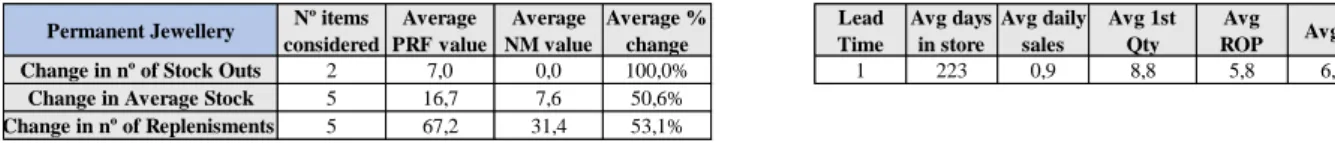
Table 1: Comparative analysis of the set of Permanent Jewellery items in Colombo store.
Regarding the permanent jewellery cluster in Colombo store, the results shown in table 1 demonstrate that in average, the in-store inventory is excessively high, and that it can be reduced in an average absolute value of less 9,1 items, for the set of five items selected. By eliminating the existing stock breaks, it is also possible to reduce in approximately 36 the average number of replenishments, for the time period considered.
Table 2: Comparative analysis of the set of Fashion Jewellery items in Colombo store.
For the set of fashion jewellery items, by reducing 100% of the stock out occurrences, the in-store stock can be reduced in an average of 1,2 items. A lower value than the one obtained for the permanent items was already expected, since both set of items present different profiles in a store. That is, fashion items are the newness of the season, and therefore, it is uncommon (specially for the set of best sellers selected) to accumulate excess in-store stock. As it can be seen in table 2, the average number of replenishments also presents a lower reduction when compared to the permanent cluster mostly due to the differences in the time period considered. In addition, the higher value obtained for the permanent items' average daily sales is also
Permanent Jewellery Nº items considered Average PRF value Average NM value Average % change Lead Time Avg days in store Avg daily sales Avg 1st Qty Avg ROP Avg Q
Change in nº of Stock Outs 2 7,0 0,0 100,0% 1 223 0,9 8,8 5,8 6,6
Change in Average Stock 5 16,7 7,6 50,6%
Change in nº of Replenisments 5 67,2 31,4 53,1%
Fashion Jewellery Nº items considered Average PRF value Average NM value Average % change Lead Time Avg days in store Avg daily sales Avg 1st Qty Avg ROP Avg Q
Change in nº of Stock Outs 2 6,5 0,0 100,0% 1 82 0,5 13,2 4,2 5,0
Change in Average Stock 5 7,2 6,0 15,1%
20 responsible for the discrepancy observed in the number of replenishments made. Since fashion items showed a lower volume of sales per day, it is likely to cause a reduction in replenishments. Moreover, the average point at which reorders are placed for the fashion set of items is also lower: it will take longer for a replenishment to be placed when compared to the permanent set of items.
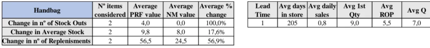
Table 3: Comparative analysis of the set of Handbag items in Colombo store.
The results observed in table 3 for the two handbag items show similarities to the previous set of items. Although the two items are seasonal, its average life-cycle is closer to the set of permanent jewellery items selected. Nevertheless, its seasonality is responsible for an average absolute in-store change value of 1,8, identical to the same parameter value obtained for the set of fashion jewellery items. The average reduction in the number of replenishments made is closer to the permanent jewellery value obtained, which is also mainly related to the proximity of the in-store duration, as well as the average daily sales values.
Table 4: Comparative analysis of the set of all items in Colombo store.
In general, for the set of twelve items analysed from the Colombo store, by considering an average sale of 0,8 items per day, the new model sets an average reorder point of 5,1 items. Subsequently, ordering the average quantity of 6,0 items eliminates 35 stock breaks. This reduces the store stock by 30,3% on average, which means 4,6 items less when compared to the in-store inventory verified through the Parfois’ system, for the set of items considered, as seen in table 4. This suggests that the unnecessary in-store stock at Parfois’ retail stores is unable to cover the existing stock breaks. Therefore, the product provided to stores may not be the right product to satisfy consumers’ demand. Moreover, the Parfois’ system of replenish in the face of an ideal quantity, originates a massive quantity of shipments that can be reduced by 50,2% with
Handbag Nº items considered Average PRF value Average NM value Average % change Lead Time Avg days in store Avg daily sales Avg 1st Qty Avg ROP Avg Q
Change in nº of Stock Outs 2 4,0 0,0 100,0% 1 205 0,8 9,0 5,5 7,0
Change in Average Stock 2 9,8 8,0 17,6%
Change in nº of Replenisments 2 56,5 24,5 56,9% TOTAL Nº items considered Average PRF value Average NM value Average % change Lead Time Avg days in store Avg daily sales Avg 1st Qty Avg ROP Avg Q
Change in nº of Stock Outs 6 5,8 0,0 100,0% 1 161 0,8 10,7 5,1 6,0
Change in Average Stock 12 11,6 7,0 30,3%
21 the new model for the set of items considered. This reduction means almost a month’s worth of shipments for the almost six months period considered.
• Warszawa Zlote Tarasy store:
Table 5: Comparative analysis of the set of Fashion Jewellery items in Warszawa Zlote Tarasy store.
In what concerns the set of the three fashion jewellery items selected, under the new model, it is possible to decrease by 72,2% the average number of replenishments made, which prompts a reduction of approximately 20 shipments. At the same time, table 5 shows that the average number of in-store stock increases by 0,9 items for the sample of three items taken. This means that, in this case, the new model enables a reduction of the average number of shipments by increasing the quantity of order of each replenishment.
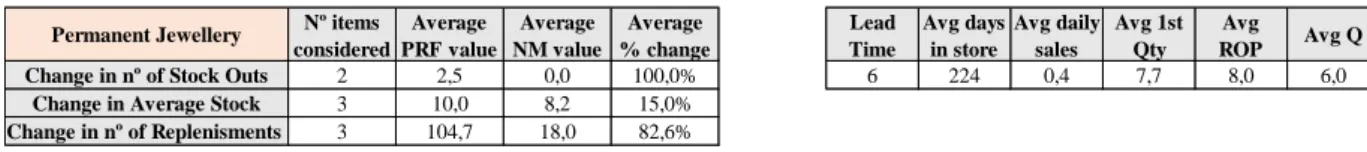
Table 6: Comparative analysis of the set of Jewellery Permanent items in Warszawa Zlote Tarasy store.
From the permanent set of items, the value parameter that stands out is the average number of shipments performed, as seen in table 6. As mentioned above, under the Parfois’ system, the number of orders is expected to be always higher than the value obtained from the model used. In the polish market, the new model defines that a replenishment of an item occurs whenever the in-store stock is at or below a set reorder point and if no order is placed during the six previous days. Thus, the new approach will always suggest less replenishments than a system that responds directly to sales. In comparison to the set of fashion items, as explained for Colombo’ set of items, the longer time period considered is the main cause for the value of replacements obtained, a reduction of approximately 87 replenishments.
Fashion Jewellery Nº items considered Average PRF value Average NM value Average % change Lead Time Avg days in store Avg daily sales Avg 1st Qty Avg ROP Avg Q
Change in nº of Stock Outs 2 1,5 0,0 100,0% 6 113 0,2 5,0 5,0 4,3
Change in Average Stock 3 4,4 5,3 -31,6%
Change in nº of Replenisments 3 27,3 6,0 72,2%
Permanent Jewellery Nº items considered Average PRF value Average NM value Average % change Lead Time Avg days in store Avg daily sales Avg 1st Qty Avg ROP Avg Q
Change in nº of Stock Outs 2 2,5 0,0 100,0% 6 224 0,4 7,7 8,0 6,0
Change in Average Stock 3 10,0 8,2 15,0%
22
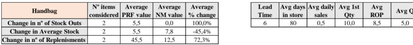
Table 7: Comparative analysis of the set of Handbag items in Warszawa Zlote Tarasy store.
The two handbag items considered present a similar scenario to the set of fashion jewellery items which implies a reduction in the number of replenishments performed by increasing the quantity of replenishment, as a consequence of the elimination of the total existing stock breaks (see table 7).
Table 8: Comparative analysis of the set of Handbag items in Warszawa Zlote Tarasy store.
For the set of eight items selected from Warszawa Zlote Tarasy, for an average sale of 0,4 items per day, the model defines an average point of order of 7,0 items. The average order quantity of 5,1 items avoids approximately 19 stock breaks. This results in an average reduction of 77% in replacements, achieved by increasing the in-store inventory in approximately 20% as table 8 shows. The large reduction is due to Parfois’ system which by responding directly to sales is able to replenish between 4 and 6 times a week. Thus, in the Polish market, where an order takes six days to arrive at the store, if a specific item is sold every day, the company’ system will suggest replenishing the sold quantity each day.
As shown in the Colombo and Warszawa stores example, the results obtained under the new model demonstrate that it is possible to improve the current replenishment system at Parfois. Both markets showed distinct results which reveals that Portugal and Poland have different needs, as a consequence of different characteristics. However, the model addressed each market and provided opportunities for improvement in both, offering a higher accuracy of inventory in retail stores through the elimination of all existing stock breaks. In addition, the company’s logistics processes may also be optimized by decreasing the number of shipments performed. As
Handbag Nº items considered Average PRF value Average NM value Average % change Lead Time Avg days in store Avg daily sales Avg 1st Qty Avg ROP Avg Q
Change in nº of Stock Outs 2 5,5 0,0 100,0% 6 80 0,5 10,0 8,5 5,0
Change in Average Stock 2 5,5 7,8 -45,4%
Change in nº of Replenisments 2 45,5 12,5 72,3% TOTAL Nº items considered Average PRF value Average NM value Average % change Lead Time Avg days in store Avg daily sales Avg 1st Qty Avg ROP Avg Q
Change in nº of Stock Outs 6 3,2 0,0 100,0% 6 157 0,4 7,3 7,0 5,1
Change in Average Stock 8 6,7 7,3 -19,5%
23 a result, positive outcomes in cost efficiency can be achieved when extending the new model to the Parfois’ world of products.
6.1 Parfois’ Implementation Proposal
The improvement perceived led the present work project to suggest how the model could be implemented in the context of Parfois, as a proposal for a new item-store approach.
In this way, a forecast of the variables of the model was performed for the sample. Under the new proposal, the average point at which reorders should be placed, the average quantity to send for the first shipment and the average order quantity of each replenishment are defined for each selected store, by each subcategory of product. The values presented in table 9 are a representation of the variables of the model, related to the past season’s sales of each respective subcategory. The use of a subset of counterparts to forecast items’ sales behaviour must be adjusted to the corresponding desired time period. The forecast indicators are essentially used for the beginning of the item’s life cycle, as well as for peak of sales, in order to predict sales more accurately.
Table 9: The new proposal forecast indicators
In this proposal, the item is tracked after it is sent to the store for the first time and the variables of the model must be adjusted on a daily basis. That is, the performance of each item regarding the past days’ sales must be taken into account, as it is done in the current Parfois’ system. Since the reorder point is the variable that can reflect sales’ behaviour through the average daily sales, the number of items purchased per shopper, as well as the number of shoppers per day – it is this variable which must fluctuate. Accordingly, in this new approach, the point at which reorders should be placed will increase or decrease as a reflection of sales. Therefore, the new approach must be accompanied by an ongoing process to accurately respond to sales behaviour. Additionally, the ‘acceptable’ probability of out-of-stock (π) must be adjusted according to the
Store Fashio type Family Nº items considered
Avg 1st
Qty Avg ROP Avg Q
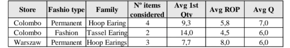
Colombo Permanent Hoop Earing 4 9,3 5,8 7,0
Colombo Fashion Tassel Earing 2 14,0 4,5 6,0
24 performance of each item in the store. This ensures the right level of inventory without unnecessary stock at retail stores, while the stock out probability of each item is controlled by the replenishment system. Although the sales seasons were not accounted in the performed analysis, and since the forecast of those periods under the Parfois’ system is mainly done by the increment of multipliers (based on the corresponding period of the previous year) the new approach proposes to do so in the same way: by increasing the value of the reorder point based on past seasons’ sales for each subcategory of items.
Even though positive results were obtained as discussed in Section 6, the new proposal would need to be tested in each item-store situation to fully assess its advantages in the Parfois’ context.
7. Limitations and Conclusions
Fast fashion is an unpredictable business model where new trends are always coming and going. In such extremely dynamic environment, it is very difficult to accurately predict sales. Therefore, there will always be room for improving the replenishment system of an ever-changing product. According to the new model, the replenishment system defines a minimum in-store level of stock – the reorder point – for which the probability of stock out is known and can be controlled. To implement the proposal that this work project puts forward, this point of order would be adjusted through the distinct variables of the model to better reflect the behaviour of sales.
As discussed throughout this thesis, the alternative approach to the company’s replenishment system was successfully applied to the selected heterogenic sample. Several limitations were identified. Firstly, the selected sample only represents a fraction of the Parfois’ world of products. Secondly, as mentioned in Section 5.1, the model takes into account the fact that a single shopper is not expected to purchase more than one or two items of the same reference and therefore, it classifies items-per-shopper as a Logarithmic probability distribution. However, the model does not account for a reference which does not exhibit more than one item purchased per shopper (at least per one shopper). Accordingly, the distribution items-per-shopper will only
25 present frequency values for f1, and consequently, the standard deviation of items-per-shopper distribution will be equal to zero. As a result, it is not possible to estimate the negative binomial parameters which are used to determine the reorder point. Thirdly, and since the rate at which shoppers enter the store is assumed to be relatively constant over time, the new model does not consider atypical periods such as sales seasons, which implies an effective assessment of the application of the new proposal to sales season periods presented in 6.2. Lastly, the volatile business model in which Parfois operates intensifies the constrains which derive from the new model proposal.
The implementation of the new proposal could bring great advantages for the company regarding the accuracy of inventory in retail stores, as well as in terms of logistics and costs reduction. The large decrease of replenishments verified could be significantly higher if the model were to be applied to a much wider sample. Although it was not possible to obtain information about the individual cost of each item selected, it is expected that a larger sample of data would confirm the benefit of costs reduction for the company. In addition, this proposal may provide a solid basis for the continuation of the company’s past project related to the incorporation of the out-of-stock rate of items in its replenishment system.
In conclusion, the present work project offers a new proposal for the current company’ stock replenishment system which would add significant value to Parfois.
8. References
Barnes, Liz, and Gaynor Lea-Greenwood. 2006. “Fast Fashioning the Supply Chain: Shaping the Research Agenda.” Journal of Fashion Marketing and Management: An International Journal 10 (3): 259–71. doi:10.1108/13612020610679259.
Christopher, Martin, Robert Lowson, and Helen Peck. 2004. “Creating Agile Supply Chains in the Fashion Industry.” International Journal of Retail & Distribution Management 32 (8): 367–76. doi:10.1108/09590550410546188.
26 Čiarnienė, Ramunė, and Milita Vienažindienė. 2014. “Agility and Responsiveness Managing Fashion Supply Chain.” Procedia - Social and Behavioral Sciences 150: 1012–19. doi:10.1016/j.sbspro.2014.09.113.
Evans, T.C., Gavrilovich, E., Mihai, R.C. and Isbasescu, I., Easyg Llc, Darryl Thelen, J A Martin, S M Allen, and Slane SA. 2017. “( 12 ) Patent Application Publication ( 10 ) Pub . No .: US 2006 / 0222585 A1 Figure 1” 002 (15): 354. doi:10.1037/t24245-000.
Kang, Yun, and Stanley B. Gershwin. 2005. “Information Inaccuracy in Inventory Systems: Stock Loss and Stockout.” IIE Transactions (Institute of Industrial Engineers) 37 (9): 843–59. doi:10.1080/07408170590969861.
Nenni, Maria Elena, Luca Giustiniano, and Luca Pirolo. 2013. “Demand Forecasting in the Fashion Industry: A Review.” International Journal of Engineering Business Management 5 (SPL.ISSUE). doi:10.5772/56840.
Thomassey, Sébastien. 2014. “Intelligent Fashion Forecasting Systems: Models and Applications.” In Intelligent Fashion Forecasting Systems: Models and Applications, 9–28. doi:10.1007/978-3-642-39869-8.
27 9. Appendices
Appendix 1 – Product Trajectory
A new season begins when designers from different categories (jewellery, handbags, apparel, footwear, and hair accessories for example) present the product to each respective purchasing department, who must choose the set of items to incorporate in the new collection according to the stipulated budget. After defining the collection plan, purchasers are in charge of ‘betting’ on the product: they decide on the quantity of items that must be purchased. There are four different levels of bet: M3, M2, M1 and SB (Super Bet), from the lowest to the highest. If purchasers bet SB on a specific subcategory, it means that they believe the item is highly commercial and therefore, it will be a best seller. In contrast, when there is a huge uncertainty related with the performance of a subcategory, i.e., because it is too trendy, purchasers would bet M3.
After product betting, the production order is sent to at least two of the manufacturers, in China, India or Cambodia. The manufacturing process is followed by the company until the product arrives in Portugal. The collection is shipped according to each market lead time, starting from the long-transit to the short-transit markets. The first shipment quantity follows a distinct procedure than the one used in the replenishment system. It is based on a matrix of quantities which consists of an algorithm that forecasts the initial quantity of each item to send to each store, based on the historical data of a counterpart (identical item), by subcategory of product. It is stipulated that no more than 60% of the total quantity of a new collection is sent in the first shipment in order to keep at least 40% of the stock in the warehouse for future replenishments.
Appendix 2 – POS data
Data from one selected item (119148_TKU) is used in the following appendix, as well as in Appendix 9.
Appendix 2A – Daily sales, Number of shoppers per day, Number of items purchased by each shopper on each day
28 For a specific reference (119148_TKU) during a specific time period considered
Time period
considered Daily sales
Time period
w/ sales Shoppers per Day
Items- per-Shopper 21/02/2018 0 2018-02-24 1G1X-246663 2 22/02/2018 0 2018-02-25 1G2Z-2866 1 23/02/2018 0 2018-02-26 1G2X-273960 1 24/02/2018 2 2018-02-27 1G2X-274159 1 25/02/2018 1 2018-02-28 1G2X-274356 1 26/02/2018 1 2018-03-01 1G1X-246879 1 27/02/2018 1 2018-03-01 1G2X-274646 1 28/02/2018 1 2018-03-01 1G2X-274668 1 01/03/2018 3 2018-03-02 1G3X-79851 1 02/03/2018 1 2018-03-03 1G1X-246946 1 03/03/2018 1 2018-03-04 1G2X-275329 1 04/03/2018 1 2018-03-05 1G1X-247111 1 05/03/2018 2 2018-03-05 1G2X-275492 1 06/03/2018 1 2018-03-06 1G2X-275718 1 07/03/2018 1 2018-03-07 1G2X-275738 1 08/03/2018 0 2018-03-09 1G2X-276283 1 09/03/2018 1 2018-03-10 1G2X-276495 1 10/03/2018 3 2018-03-10 1G2X-276512 1 11/03/2018 2 2018-03-10 1G2X-276547 1 12/03/2018 0 2018-03-11 1G1X-247314 1 13/03/2018 0 2018-03-11 1G2X-276605 1 14/03/2018 1 2018-03-14 1G1X-247409 1 15/03/2018 2 2018-03-15 1G2X-277306 1 16/03/2018 1 2018-03-15 1G2X-277366 1 17/03/2018 0 2018-03-16 1G1X-247463 1 18/03/2018 0 2018-03-19 1G2X-278339 1 19/03/2018 1 2018-03-20 1G2X-278445 1 20/03/2018 3 2018-03-20 1G2X-278458 1 21/03/2018 2 2018-03-20 1G2X-278518 1 22/03/2018 1 2018-03-21 1G2X-278593 1 23/03/2018 3 2018-03-21 1G2X-278686 1 24/03/2018 3 2018-03-22 1G2X-278879 1 25/03/2018 0 2018-03-23 1G2X-278957 1 26/03/2018 0 2018-03-23 1G2X-279099 1 27/03/2018 1 2018-03-23 1G2X-279146 1 28/03/2018 0 2018-03-24 1G2X-279204 1 29/03/2018 3 2018-03-24 1G2X-279220 2 30/03/2018 4 2018-03-27 1G2X-280062 1 31/03/2018 0 2018-03-29 1G2X-280437 1 01/04/2018 0 2018-03-29 1G2X-280533 1 02/04/2018 0 2018-03-29 1G2X-280592 1 03/04/2018 0 2018-03-30 1G1X-248019 1
29 04/04/2018 0 2018-03-30 1G2X-280762 1 05/04/2018 1 2018-03-30 1G2X-280801 1 06/04/2018 2 2018-03-30 1G2X-280855 1 07/04/2018 2 2018-04-05 1G2X-281968 1 08/04/2018 1 2018-04-06 1G2X-282277 1 09/04/2018 1 2018-04-06 1G2X-282289 1 10/04/2018 2 2018-04-07 1G1X-248351 1 11/04/2018 3 2018-04-07 1G2X-282421 1 12/04/2018 0 2018-04-08 1G2X-282588 1 13/04/2018 1 2018-04-09 1G2X-282956 1 14/04/2018 1 2018-04-10 1G2X-283071 1 15/04/2018 0 2018-04-10 1G2X-283137 1 16/04/2018 0 2018-04-11 1G1X-248468 1 17/04/2018 0 2018-04-11 1G2X-283270 1 18/04/2018 0 2018-04-11 1G2X-283298 1 19/04/2018 0 2018-04-13 1G2X-283641 1 20/04/2018 0 2018-04-14 1G2X-283879 1 21/04/2018 0 2018-04-25 1G2X-286249 1 22/04/2018 0 2018-04-27 1G2X-286644 1 23/04/2018 0 2018-04-28 1G2Z-3243 1 24/04/2018 0 2018-04-29 1G2X-287276 1 25/04/2018 1 2018-04-29 1G2X-287280 1 26/04/2018 0 2018-04-30 1G2X-287548 1 27/04/2018 1 2018-05-01 1G1X-249523 1 28/04/2018 1 2018-05-05 1G1X-249856 1 29/04/2018 2 2018-05-06 1G1X-250087 1 30/04/2018 1 2018-05-06 1G1X-250112 1 01/05/2018 0 2018-05-06 1G2X-289044 1 02/05/2018 0 2018-05-09 1G2X-289621 1 03/05/2018 0 2018-05-09 1G2X-289726 1 04/05/2018 0 2018-05-09 1G2X-289739 1 05/05/2018 1 2018-05-09 1G2X-289745 1 06/05/2018 3 2018-05-09 1G2Z-3422 1 07/05/2018 0 2018-05-10 1G2X-289823 1 08/05/2018 0 2018-05-11 1G1X-250425 1 09/05/2018 5 2018-05-12 1G2X-290399 1 10/05/2018 1 2018-05-13 1G1X-250577 1 11/05/2018 1 2018-05-14 1G1X-250619 1 12/05/2018 1 2018-05-14 1G2X-290831 1 13/05/2018 1 2018-05-14 1G2X-290937 1 14/05/2018 3 2018-05-15 1G2X-291016 1 15/05/2018 2 2018-05-15 1G2X-291179 1 16/05/2018 2 2018-05-16 1G1X-250728 1 17/05/2018 1 2018-05-16 1G1X-250865 1 2018-05-17 1G2X-291303 1
30 Appendix 2B – Average daily sales and Items-per-shopper Histogram
Appendix 2C – Average Items-per-shopper and Standard deviation of Items-per-shopper
Appendix 2D – Average shoppers per day, Single-store multi-day sales model and Negative Binomial parameters (p, k)
Appendix 2E – Maximal volume of sales, Next lowest probability, Acceptable probability initially defined
Appendix 2E – Reorder point
Avg daily sales
1,02 Xi fi fi/Sum fi Xi*(fi/Sum fi)
1 85 0,98 0,98 2 2 0,023 0,046 Items-per-shopper Histogram μ 1,02 σ 0,15 λ λ*(L+1) 1,00 2,00 p 0,96 k 45,53 x Stock Out % π 0 86,49% 1% 1 60,04% 1% 2 33,56% 1% 3 15,52% 1% 4 6,10% 1% 5 2,09% 1% 6 0,63% 1% 7 0,17% 1% 8 0,04% 1% 9 0,01% 1% 10 0,00% 1% 6 ROP
31 Appendix 3 – Items-per-shopper distribution
The mean and standard deviation of the Xi distribution are:
Mean = E(𝑋𝑖) = μ
Variance = V(𝑋𝑖) = σ2
Appendix 4 – Average daily sales and Shoppers per day
The sum of all products purchased on a given day t by the N shoppers is equal to daily sales: 𝑆𝑡= 𝑋𝑖+ ⋯ + 𝑋𝑁
The sum of all random variables (Xi) gives the number of shoppers per day (λ). The mean and
variance of 𝑆𝑡 can be written in terms of the mean and variance of the 𝑋𝑖 as:
Mean = E(𝑆𝑡) = λμ
Variance = V(𝑆𝑡) = λ(σ2+ 𝜇2)
By rearranging the relationship, the number of shoppers per day is:
𝜆 =E(𝑆𝑡) μ Appendix 5 – Logarithmic Distribution
The Logarithmic density function is:
𝑓𝑗= Pr(𝑋𝑖= 𝑗) = 𝑐 𝑞 𝑗 𝑗 𝑐 = − 1 ln (1 − 𝑞) 0 < 𝑞 < 1 𝑗 𝜖 {1,2, . . . }
The density function decreases as j increases. For small values of the parameters q, the decrease is steep. The limiting case is the exclusively-one-item-per-shopper situation:
lim
𝑞→0𝑓(𝑋𝑖) =
1 𝑗 = 1 0 𝑗 > 1
Appendix 6 – Negative Binomial Parameters The Negative Binomial distribution is defined below:
32 Pr(X = x) = P(k + x) P(k) P(x + 1) p k(1 − p) x ∈ {0,1, 2,…} k ≥ 0 0 < p <1
The mean and variance are defined by the equations:
Mean = E(X) = k1 − p p Variance = V(X) = k1 − p
p2 Solving for k and p in terms of the mean and variance gives:
p =E(x) V(x)
k = (E(x))
2
V(x) − E(x)
By substituting the mean and variance of 𝑆𝑡 for E(X) and V(X) respectively gives the
Method-of-Moments fit of the Negative Binomial to the distribution of 𝑆𝑡, which defines p and k as:
p = λμ λ(σ2+ μ2) = μ σ2+ μ2 k = (λμ) 2 λ(σ2+ μ2) − λμ = λμ2 σ2+ μ2− μ
33 Appendix 7 – Selected Sample
The selected sample of items is shown in the following table:
Country Store Category Fashion Type Subcategory Reference
Portugal Centro Comercial Colombo Jewellery Fashion Tassel 149693_PUU
Tassel 158517_BMU
Stud 119148_TKU
Drop 158833_BMU
Dangle 1309622HMU
Jewellery Permanent Hoop 138911_GDU
Hoop 160206_SVU
Hoop 1601861SVU
Hoop 160186_GDU
Drop 160202_BGU
Handbag Fashion Backpack 154247_BKM
Shopper 154952_CAL
Poland WARSZAWA Zlote Tarasy Jewellery Fashion Tassel 149693_PUU
Stud 119148_TKU
Drop 158818_PMU
Jewellery Permanent Hoop 138911_GDU
Hoop 160172_GDU
Hoop 160161_GDU
Handbag Fashion Cross 156359_LGM
34 Appendix 8 – Comparison Mechanism
Appendix 8B – New Model Data Appendix 8D – Parfois Data
Time period considered In-store Stock beginning day Daily sales In- store Stock end day
Replenishments Date SOH SIT
STK total (only for accuracy) 21/02/2018 14 0 14 0 20/02/2018 0 14 14 22/02/2018 14 0 14 0 21/02/2018 14 0 14 23/02/2018 14 0 14 0 22/02/2018 14 0 14 24/02/2018 14 2 12 0 23/02/2018 12 0 12 25/02/2018 12 1 11 0 24/02/2018 11 0 11 26/02/2018 11 1 10 0 25/02/2018 10 0 10 27/02/2018 10 1 9 0 26/02/2018 9 0 9 28/02/2018 9 1 8 0 27/02/2018 8 1 9 01/03/2018 8 3 5 0 28/02/2018 6 0 6 02/03/2018 5 1 4 6 01/03/2018 5 8 13 03/03/2018 4 1 3 0 02/03/2018 4 8 12 04/03/2018 9 1 8 0 03/03/2018 3 8 11 05/03/2018 8 2 6 0 04/03/2018 1 10 11 06/03/2018 6 1 5 6 05/03/2018 8 6 14 07/03/2018 5 1 4 0 06/03/2018 7 7 14 08/03/2018 10 0 10 0 07/03/2018 12 2 14 09/03/2018 10 1 9 0 08/03/2018 13 1 14 10/03/2018 9 3 6 0 09/03/2018 10 1 11 11/03/2018 6 2 4 6 10/03/2018 8 1 9 12/03/2018 4 0 4 0 11/03/2018 8 1 9 13/03/2018 10 0 10 0 12/03/2018 9 6 15 14/03/2018 10 1 9 0 13/03/2018 8 6 14 15/03/2018 9 2 7 0 14/03/2018 12 0 12 16/03/2018 7 1 6 0 15/03/2018 11 2 13 17/03/2018 6 0 6 6 16/03/2018 11 2 13 18/03/2018 6 0 6 0 17/03/2018 11 2 13 19/03/2018 12 1 11 0 18/03/2018 12 0 12 20/03/2018 11 3 8 0 19/03/2018 9 0 9 21/03/2018 8 2 6 0 20/03/2018 7 4 11 22/03/2018 6 1 5 6 21/03/2018 10 0 10 23/03/2018 5 3 2 0 22/03/2018 7 0 7 24/03/2018 8 3 5 0 23/03/2018 4 0 4 25/03/2018 5 0 5 6 24/03/2018 4 0 4 26/03/2018 5 0 5 0 25/03/2018 4 15 19 27/03/2018 11 1 10 0 26/03/2018 18 0 18 28/03/2018 10 0 10 0 27/03/2018 18 0 18 29/03/2018 10 3 7 0 28/03/2018 15 0 15 30/03/2018 7 4 3 0 29/03/2018 11 0 11 31/03/2018 3 0 3 6 30/03/2018 11 0 11
35 01/04/2018 3 0 3 0 31/03/2018 11 0 11 02/04/2018 9 0 9 0 01/04/2018 11 3 14 03/04/2018 9 0 9 0 02/04/2018 14 0 14 04/04/2018 9 0 9 0 03/04/2018 14 0 14 05/04/2018 9 1 8 0 04/04/2018 13 1 14 06/04/2018 8 2 6 0 05/04/2018 12 0 12 07/04/2018 6 2 4 6 06/04/2018 10 0 10 08/04/2018 4 1 3 0 07/04/2018 9 0 9 09/04/2018 9 1 8 0 08/04/2018 8 0 8 10/04/2018 8 2 6 0 09/04/2018 6 0 6 11/04/2018 6 3 3 6 10/04/2018 3 0 3 12/04/2018 3 0 3 0 11/04/2018 3 0 3 13/04/2018 9 1 8 0 12/04/2018 2 0 2 14/04/2018 8 1 7 0 13/04/2018 1 0 1 15/04/2018 7 0 7 0 14/04/2018 1 0 1 16/04/2018 7 0 7 0 15/04/2018 1 0 1 17/04/2018 7 0 7 0 16/04/2018 1 0 1 18/04/2018 7 0 7 0 17/04/2018 1 0 1 19/04/2018 7 0 7 0 18/04/2018 1 13 14 20/04/2018 7 0 7 0 19/04/2018 14 0 14 21/04/2018 7 0 7 0 20/04/2018 14 0 14 22/04/2018 7 0 7 0 21/04/2018 14 0 14 23/04/2018 7 0 7 0 22/04/2018 14 0 14 24/04/2018 7 0 7 0 23/04/2018 14 0 14 25/04/2018 7 1 6 0 24/04/2018 13 0 13 26/04/2018 6 0 6 6 25/04/2018 13 0 13 27/04/2018 6 1 5 0 26/04/2018 12 0 12 28/04/2018 11 1 10 0 27/04/2018 11 0 11 29/04/2018 10 2 8 0 28/04/2018 9 0 9 30/04/2018 8 1 7 0 29/04/2018 8 0 8 01/05/2018 7 0 7 0 30/04/2018 8 0 8 02/05/2018 7 0 7 0 01/05/2018 8 2 10 03/05/2018 7 0 7 0 02/05/2018 10 1 11 04/05/2018 7 0 7 0 03/05/2018 11 0 11 05/05/2018 7 1 6 0 04/05/2018 10 0 10 06/05/2018 6 3 3 6 05/05/2018 7 0 7 07/05/2018 3 0 3 0 06/05/2018 7 2 9 08/05/2018 9 0 9 0 07/05/2018 9 0 9 09/05/2018 9 5 4 0 08/05/2018 4 0 4 10/05/2018 4 1 3 6 09/05/2018 3 9 12 11/05/2018 3 1 2 0 10/05/2018 11 0 11 12/05/2018 8 1 7 0 11/05/2018 10 0 10 13/05/2018 7 1 6 0 12/05/2018 9 0 9 14/05/2018 6 3 3 6 13/05/2018 6 0 6 15/05/2018 3 2 1 0 14/05/2018 4 1 5 16/05/2018 7 2 5 0 15/05/2018 3 0 3 17/05/2018 5 1 4 6 16/05/2018 2 0 2
36 Appendix 8A – First shipment quantity
Appendix 8C – Optimal order quantity
Appendix 8D – New Model (NM) vs. Parfois’ System (PRF)
Appendix 9 – Comparative Analysis
The results obtained by the same analysis for each the remaining items from the selected sample are shown below:
Colombo Store:
• Fashion Jewellery item - 149693_PUU 14
1st Shipment Q
2
Order Q Nº Stock Outs Avg In-Store Stock Nº replenishments
2 36 1,79 36 3 3 5,05 26 4 2 5,58 20 5 1 5,92 16 6 0 6,58 14 7 0 7,29 12 8 0 7,16 10 9 0 7,73 9 Minimum Displayed Q
Order Q Nº Stock Outs Avg In-Store Stock Nº replenishments
6 0 6,58 14
Ideal Stock Nº Stock Outs Avg In-Store Stock Nº Replenishments
PRF STKi 0 8,57 27 x Stock Out % π 4 0 42,83% 1% 17 1 15,76% 1% 2 5,43% 1% 3 1,80% 1% 4 0,58% 1% 5 0,19% 1% 6 0,06% 1% 7 0,02% 1% 8 0,01% 1% 9 0,00% 1% 1st Shipment Q ROP
37 • Fashion Jewellery item - 158833_BMU
• Fashion Jewellery item - 158517_BMU
2
Order Q Nº Stock Outs Avg In-Store Stock Nº replenishments
3 7 5,10 13 4 3 5,46 10 5 3 6,75 8 6 1 5,83 7 7 3 7,69 6 8 1 8,56 5 9 0 6,36 5 10 0 9,30 4 Minimum displayed Q
Ideal Stock Nº Stock Outs Avg In-Store Stock Nº Replenishments
PRF STKi 1 6,44 16 x Stock Out % π 3 0 49,96% 1% 12 1 16,45% 1% 2 4,14% 1% 3 0,86% 1% 4 0,16% 1% 5 0,03% 1% 6 0,00% 1% 1st Shipment Q ROP 2
Order Q Nº Stock Outs Avg In-Store Stock Nº Replenishments
1 14 3,26 21 2 2 4,60 11 3 1 4,48 7 4 0 5,81 6 5 1 6,61 5 6 0 7,03 4 7 0 5,28 3 Minimum Displayed Q
Ideal Stock Nº Stock Outs Avg In-Store Stock Nº Replenishments
PRF STKi 12 5,75 32
ROP Stock Out % π 5
0 74,04% 1% 11 1 40,01% 1% 2 16,76% 1% 3 5,74% 1% 4 1,68% 1% 5 0,43% 1% 6 0,10% 1% 7 0,02% 1% 8 0,00% 1% ROP 1st Shipment Q