Control and Model Identification of a Mobile Robot's Motor based in Least Squares and Instrumental Variable methods

Texto

(1)MMAR 11th IEEE International Conference on Methods and Models in Automation and Robotics ê Poland 2 0 0 5 29 August - 1 September 2005, Miedzyzdroje,. Control and Model Identification of a Mobile Robot’s Motors based in Least Squares and Instrumental Variable Methods. Andr´e Scolari Concei¸c˜ao1 , Paulo J. Costa and A. Paulo Moreira Department of Electrical and Computer Engineering University of Porto - Porto - Portugal. [scolari,paco,amoreira]@fe.up.pt. Abstract. When no exact measurements are available the task of solving the differential equations describing the dynamics of mobile robot can be hard and inefficient. In this paper we propose a procedure for dynamic model identification and control of the process (motor + reduction + encoder) of a omni-Directional Mobile Robot’s Motors. Our techniques are based in Least Squares Methods and Instrumental Variable Methods for linear dynamic systems. Notably, the approach used here is applicable to any robot with DC motors, or, more generally, to any process with DC motor with encoder and PWM control made by a microcontroller. Key Words. Dynamic model Identification, mobile robots, control systems. 1.. INTRODUCTION. In this paper we focus attention on a omnidirectional mobile robot with four motors, as shown in 1, built for the 5dpo-2005 Robotic Soccer team from the Department of Electrical and Computer Engineering at the University of Porto at Porto, Portugal. We are particularly interested in the motor+reduction+encoder process represented in Fig. 2. This process consists on the relation between the voltage and the velocities of the robot’s motors. The dynamics of this process is complex and may be nonlinear due to the mechanic architecture of the robot which may add perturbations like attrition due to the interaction between the robot components. The task of solving the differential equations modeling the dynamics of this process may be a hard one or even be inefficient not only because of the nonlinearities but also because no exact measurements of the parameters are known. The design and simulation of controllers (as for example, the discrete PID controller implemented in the microcontroller of the robot) for the navigation of the robot require the identification of a dynamic model for this process. Here we present the identification of a discrete system (see Fig. 1) for the motor+reduction+ encoder process. This is a first step towards the dynamic model identification of the whole robot. We. consider a discrete linear model and we use techniques based on Least Square Methods and Instrumental Variable methods to estimate a transfer function for the process. This procedure is not only confined to our mobile robot. It can be applied to any robot with DC motors, or, more generally, to any process with DC motor with encoder and PWM control made by a microcontroller.. Figure 1: Mobile robot - motors.. Figure 2: Discrete dynamic system. The robot’s control and communication structure is as sketched in Fig. 3. The computer (PC) controls all the actions of the robot. The communication with the microcontroller is done through the serial port (RS232). It controls the motors using signals of PWM and a drive of power. The. 1 Supported by the Program Alβan, the European Union Program of High Level Scholarships for Latin America, scholarship n.E04D028256BR. IEEE Conference Number: 10351. 479.

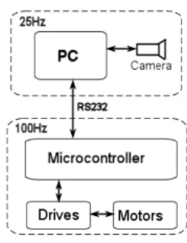
(2) software of control in PC works in a frequency of 25Hz, from the camera. However, and in order to control efficiently the motors of the robot, the microcontroller has a discrete PID controller that works in a frequency of 100Hz.. where the numerator polynomial B(z) and denominator polynomial A(z) are defined as: B(z) = b0 z n + b1 z n−1 + ... + bn ,. (4). A(z) = z n + a1 z n−1 + ... + an .. (5). For the design of a computer-controlled system like the one in Fig. 2, the model (1) must describe the dynamical behavior of the control loop between the input of the D/A converter and the output of the A/D converter. A general model for a large class of single-input, single-output systems proposed in [6] and [4], is y(k) = H1 (z)u(k) + H2 (z)ξ(k),. (6). Figure 3: Robot’s control and communication structure. This paper is structured in the following way. In section 2. we give a brief description of a deterministic model and we determine a Least Square Estimator. In section 3. we apply the Least Squares estimator to the process for the motor 1 (front) of the mobile robot. An Instrumental variable estimator is presented in section 4.. The estimation results for motors 2, 3 and 4 of the mobile robot is presented in Section 5.. The design of PID controller for Robot’s Motors is showed in section 6.. Finally, the conclusion and future works is drawn in section 7... where y(k) and u(k) are the output and input sequences, respectively, and ξ(k) is a gaussian white noise sequence with variance σ 2 and zero mean. Parameterizing H1 (z) and H2 (z) respectively as B(z) 1 A(z) and A(z) where B(z) and A(z) are defined in (4) and (5), (1) can be expressed as,. 2.. where. DETERMINISTIC MODEL AND LEAST SQUARES ESTIMATOR. In general, a linear time-invariant discrete-time system with input sequence u(k) and output sequence y(k) can be represented by an nth-order difference equation relating the input and output ([3]),. A(q −1 )y(k) = B(q −1 )u(k) + ξ(k) where q is the operator of unit delay q y(k − 1) yielding −1. y(k). =. = x(k)T θ + ξ(k). θT x(k)T. y(k) = −. ai y(k − i) +. i=1. nb X. bi u(k − i),. (1). (1 + a1 z −1 + ... + an z −n ) U (z) = , Y (z) (bo + b1 z −1 + ... + bn z −n ). H(z) =. 480. Y (z) B(z) = , U (z) A(z). (3). (10). (11). where Y T = [y(1), ..., y(N )], X T = [x(1), ..., x(N )],. (12) (13). ΞT = [ξ(1), ..., ξ(N )].. (14). Applying the Least Square Method to (11) suggests that the resulting estimator for θ is, θb = [X T X]−1 X T Y. 3.. Multiplying both sides of (2) by z and rearrange it to obtain the transfer function of the discrete-time system,. (8). Equation (8) can be expressed in vector form for N samples, as. (2). n. y(k) =. = (a1 , ..., ana , b0 , ..., bnb ) (9) = (−y(k − 1), ..., −y(k − na)... u(k), ..., u(k − nb)).. i=0. where k is the time variable, and n is a fixed integer called the order of the difference equation. The Z-transform of the difference equation (1) leads to. (7). −a1 y(k − 1)... − ana y(k − na) + ... b0 u(k)... + bnb u(k − nb) + ξ(k). Y = Xθ + Ξ na X. −1. (15). APPLICATION OF LEAST SQUARES ESTIMATOR. Now we apply the excitation signal in Fig. 4(a) to the process to obtain the curve of speed of robot’s motor 1 (front), in meters per second, as is shown in Fig. 4(b)..

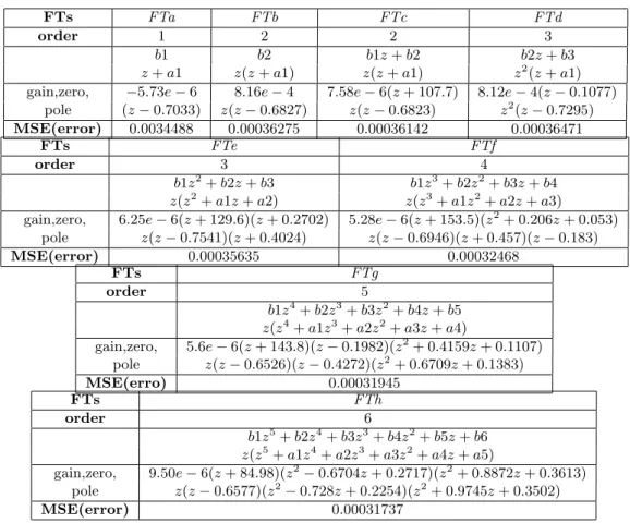
(3) 0.5. White Gaussian Noise. White gaussian noise −3. 4.5. 0.45. 250. 4. 3.5. 0.35. 200 3. 0.3. MSE(erro). speed[m/s]. 200. 150. 150. 0.25. 0.2 100. 100. 0.15. 50. 0.5. 0.05. 0. 0. 100. 150. 200. 250. samples. 300. 0. 350. 2. 1. 50. 50. 2.5. 1.5. 0.1. 0 0. x 10. 250. 0.4. 50. 100. 250. 200. 150. 300. 350. 0 0. samples. 50. a. 100. 150. samples 200. 250. 300. b. 350. c. d. e. f. g. Type. (a) Signal 1 - Gaussian (b) Curve of speed - motor white noise. 1.. (a) Signal 2 - Gaussian (b) Results of validation for white noise eight TFs. Figure 4: Signal of excitation 1 and response of motor 1. We test the efficiency of the Least Square Estimator (15) for eight different transfer functions(TF). Table 3 shows the results of the Least Squares estimation for those eight TFs: the estimation error, value of the gain, poles and zeros are presented for each TF. Fig.5(a) shows the measured and estimated speed for robot’s motor 1, with the transfer function type F T b. The estimation values can be seen in table 3. The error in table 3 is calculated by MSE (Mean Square Error),. Figure 6: Signal of excitation 2 and results of validation. Type TF order MSE(error) FTa 1 0.0042402 FTb 2 0.0010013 FTc 2 0.00099887 FTd 3 0.00099609 FTe 4 0.00099436 FTf 5 0.00099183 FTg 6 0.00099442. M SE() =. PN b 2 1 [(Φ − Φ) ] , N. (16). It calculates the sum of squared errors between b the vector of estimated speeds(Φ) b = [b Φ y (1), ..., yb(N )]T ,. and the vector of measured speeds (Φ) of the motor, Φ = [y(1), ..., y(N )]T . where N is the number of samples. 0.15. 0.2. measured speed estimated speed. measured speed simulated speed. 0.15. 0.1. 0.1. 0.05 0.05. 0 0. −0.05 −0.05. −0.1 −0.1. −0.15. −0.20. −0.15. 50. 100. 150. 200. 250. samples. 300. −0.20. 50. 100. 150. 200. 250. 300. samples. (a) Measured and esti- (b) Measured and estimated speeds with F T b - mated speeds with T F b motor 1. (Validation).. Figure 5: Speeds - motor 1. 3.1.. Table 1: Results of validation for eight TFs. Analyzing the errors in the validation in table 1, we conclude that a TF type T F b, order two, is a good approximation of the process, because the system in Fig. 2 has one delay from the loop of communication, represented by the pole at the origin in transfer function T F b. The process of DC motor can be approximated by one first-order system, considering inductance of motor null. Notice that the error with T F g is greater that with T F f , so the best order is 5. The T F b has order two, hence it is simpler to use when designing the controller in general. Moreover the difference between the error of T F b and the others TFs is small. Taking all this into account, we chose T F b. Observe that the transfer function T F a does not have a satisfactory result. The T F d was tested to verify the estimation with two delays (two poles at the origin), but the estimation error is greater than the TFs with one delay.. VALIDATION. To validate the Least square estimation, we apply another excitation signal to the process and estimated transfer functions, shown in Fig 6(a). In Table 1 and Fig.6(b) we present the MSE of error for the eight TFs for the second excitation signal. Fig.5(b) shows the curves of measured speed and simulated speed, for the transfer function of type F T b.. 4.. INSTRUMENTAL VARIABLE. The Least Squares estimators are not in general consistent when the sequence ξ(k), in (8), is correlated. Since Instrumental variable estimators are weakly consistent (see [6]and [4]) we implemente it and compare with results from the Least Squares Estimator. Our Instrumental variable estimator is θ = [Z T X]−1 Z T Y the matrix Z being constructed using the auxiliary model Z(k)T = [−b y (k − 1), −b y (k − 2), .... (17). −b y (k − n), u(k), u(k − 1), ..., u(k − n)]. (18). 481.

(4) where. b y (k) = B(z)u(k) b A(z)b. b b In the above A(z), B(z) are polynomials in z −1 . b b A(z) and B(z) are obtained from an initial least squares fit. Table 2 presents results of estimation with Instrumental variable(IV) and Least squares(LS), for the transfer function type T F b. After three iterations, the values of poles and gain stabilize. FTs LS IV 3a Iteration b1 0.00081626 0.00081538 z(z + a1) z(z − 0.6827) z(z − 0.7051) M SE(error) 0.0010013 0.00098799 Table 2: Estimated values. Analyzing the auto-correlation of error, calculated as b cy(k − 1) + b1u(k yb(k) = −a1 − 2),. 0.6. Sample Autocorrelation. Sample Autocorrelation. 0.6. 0.4. 0.2. 0. 0.4. 0.2. 0. −0.2 0. 10. 20. 30. 40. 50 Lag. 60. 70. 80. (a) Least Squares. 90. 100. −0.2 0. 10. 20. 30. 40. 50 Lag. 0.05. 0.05. 0. 0. −0.05. −0.05. −0.1. −0.1. −0.15. −0.15. 50. 100. 150. 200. 250. 300. −0.20. 50. 100. Samples. 150. 200. 60. 70. 80. 90. 100. 250. 300. Samples. (a) Motor 1 - front wheel. (b) Motor 3 - back wheel. Figure 8: Motors 1 and 3. Measured Estimated. Sample Autocorrelation Function (ACF). 0.8. 0.1. −0.20. Measured Estimated. 0.15. 0.1. (20). where yb(k) is the output estimated, y(k) is the output measured and u(k) the input signal, we can calculate the correlation of residuals. In Fig.7 we present the auto-correlation for the estimation with Least Squares and Instrumental Variable, for 100 samples. For the Least Square estimator the mean of de error Error (k), (see (20)) is 5.2879e − 4 and for Instrumental variable estimator is 5.2554e − 4. It is possible to verify that the auto-correlation of error Error for the Least Squares estimator is similar to auto-correlation of the a white noise. This is the reason why it does not have a significant improvement when we use the Instrumental variable estimator. Sample Autocorrelation Function (ACF). Measured Estimated. 0.15. (19). Error (k) = yb(k) − y(k).. 0.8. Differences between robot’s motors estimation are not surprising. They are due to irregular distribution of the weight on base of mobile robot. The transfer function of the motor 4 has a slower pole. This is because of the position of battery on the base of the robot which adds weight to wheel 4. In Fig. 8 and 9 we present the measured and estimated speeds for robot’s motors using the transfer function type T F b.. Measured Estimated. 0.1. 0.1. 0.05. 0.05. 0. 0. −0.05. −0.05. −0.1. −0.1. −0.15. −0.15. −0.20. 50. 100. 150. Samples. 200. 250. 300. (a) Motor 2 - left wheel. 0 −0.2. 50. 100. 150. Samples. 200. 250. 300. (b) Motor 4 - right wheel. Figure 9: Motors 2 and 4. 6.. PID CONTROLLER FOR ROBOT’S MOTORS. To choose appropriated values for parameters of the PID controller (Kc , T i and T d), we use the close-loop pole locations for an nth-order plant using prototype Bessel systems (see [3]). Equation (21) shows the transfer function chosen to process, obtained from the IV estimator, detailed in section 4... (b) Instrumental variable. G(z) =. 0.00081538 b1 = (z − 0.7051) z − a1. (21). Figure 7: Auto-correlation of error. 5.. OTHERS RESULTS WITH ROBOT’S MOTORS. In the previous sections we show the procedure for transfer function estimation of the motor 1 of the mobile robot. Now, we present the estimation results of the motors 2, 3 and 4 of the mobile robot. For these motors the estimation results using LS and IV estimators are shown in table 4. The mobile robot into consideration has left and right wheels (2 and 4) larger than the front and back (1 and 3) wheels. The estimated gains of motors 2 and 4 in table 4 reflect this difference.. 482. The pole of the origin is ignored since it represents one delay from the loop of communication. The equivalent continuous of the process (21) can be calculated as in is [3]. It is G(s) = for. K , τs + 1. b1 1 + a1 1 τ= |ps|. K=. pz = eT ps ..

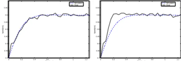
(5) where ps is the pole in S-plane and pz is the pole in Z-plane. The continuous transfer function is 0.002765 G(s) = (22) 0.1145s + 1 A PI (Proportional + Integral) controller is represented as Kc (T is + 1) Gc(s) = (23) T is We choose a PI controller (T d = 0), because the process has characteristics of a first-order system. The open-loop system GM A is Kc (T is + 1) K . T is τs + 1 (24) The close-loop system with unit feedback, from GM A (s), is. In Fig.10(a) we show the results of PI controller with the desired settling time (Ts = 0.6(seg)). In order to improve this result, we introduce a Feedforward gain f from the reference input to the process input. This gain cannot affect the stability of the control system because it does not alter the close-loop poles (see [3]). However, this gain may improve the transient response of the system. We chose the value of the parameter f to be 200, the choice being made based on simulations. Fig.10(b) shows the response of system with gain f . The reference input is a step with amplitude of 0.3(m/s) (from 0.3(m/s) to 0.6(m/s)).. GM A (s) = Gc (s).G(s) =. GM F (s) =. KKc KKc s Ti τ + τ (1+KKc )s c 2 s + + KK τ Ti τ. −(p1 + p2 ) =. (26). 0.55. 0.55. Speed[m/s]. Speed[m/s]. 0.6. 0.5. 0.5. 0.45. 0.4. 0.4. 0.35. 0.35. 0.3 0. 0.2. 0.4. 0.6 Time[seg]. 0.8. 1. 1.2. 0.3 0. 0.2. 0.4. 0.6 Time[seg]. 0.8. 1. 1.2. (a) Close-loop system with- (b) Close-loop system with out the Feedforward gain f . the Feedforward gain f .. Figure 10: Response of Close-loop system. 7.. CONCLUSION WORKS. AND. FUTURE. In this paper we identify a discrete system, shown in Fig. 2, of the a mobile robot. We use Least Squares and Instrumental Variable estimator. These estimations permit the selection of appropriate values for PI controller, implemented in the mobile robot. This is the first step for the identification of a dynamic model for the whole mobile robot considering it as a multi-variable system and using the dynamic models estimated in this work. REFERENCES 1. G.F. Franklin and J.D. Powell and M. Workman, Digital control of dynamic systems, Addison Weley Longman, Inc,1997.. and for Ti , KKc (p1 p2 ) = Ti τ KKc Ti = τ p 1 p2. Simulated Real. 0.65. 0.6. 0.45. (25). With the transfer function of the close-loop system, which is a second-order system, the procedure for choosing close-loop pole locations is as follows. Let the desired settling time be called Ts . We determine the desired settling time (Ts = 0.6seg) of the close-loop system based on performance of robot and taking into account the limitations of the system hardware. Considering the table of normalized Bessel polynomials[3], we divide the roots of the second-order polynomials p1s = −4.0530 ± j2.3400 by Ts to obtain the desired close-loop s-plane pole locations. This yields poles at p0.6s = −6.7550 ± j3.9000. The value for Kc is given by, (1 + K ∗ Kc ) τ −τ ∗ (p1 + p2 ) − 1 Kc = K. Simulated Real. 0.65. (27). 2. J.L. Martins De Carvalho, Dynamical Systems and Automatic Control, Prentice Hall, 1993.. where p1 = −6.7550+j3.9000 and p2 = −6.7550− j3.9000. The result TF is given by(28),. 3. R. J. Vaccaro, Digital Control - A State-Space Approach, McGraw-Hill, 1995.. 4.775s + 0.3747 . (28) s2 + 13.51s + 60.84 Equations (29) and (30) are, respectively, the continuous PI transfer function and the discrete PI transfer function, invariant to step responses (ZOH-zero-order hold) [1], for a sample period of 10ms: 197.68(0.07848s + 1) Gc(s) = (29) 0.07848s 197.68(z − 0.8726) Gc(z) = (30) (z − 1) GM F (s) =. 4. A. P. G. M. Moreira and P. J. G. Costa and P. J. Lopes dos Santos, Introdu¸c˜ ao ` a Identifica¸c˜ ao de Modelos Discretos para Sistemas Dinˆ amicos, Sebenta FEUP,www.fe.up.pt/amoreira, 2002. 5. K. J. Astr˜ om and T. H˜ agglund, PID controllers : Theory, design, and tuning, International Society for Measurement and Con, 1995. 6. G. C. Goodwin and R. L. Payne, Dinamic System Identification, Academic Press, 1997.. 483.

(6) FTs order. FTa 1 b1 z + a1 −5.73e − 6 (z − 0.7033) 0.0034488. FTb FTc FTd 2 2 3 b2 b1z + b2 b2z + b3 z(z + a1) z(z + a1) z 2 (z + a1) gain,zero, 8.16e − 4 7.58e − 6(z + 107.7) 8.12e − 4(z − 0.1077) pole z(z − 0.6827) z(z − 0.6823) z 2 (z − 0.7295) MSE(error) 0.00036275 0.00036142 0.00036471 FTs FTe FTf order 3 4 b1z 2 + b2z + b3 b1z 3 + b2z 2 + b3z + b4 z(z 2 + a1z + a2) z(z 3 + a1z 2 + a2z + a3) gain,zero, 6.25e − 6(z + 129.6)(z + 0.2702) 5.28e − 6(z + 153.5)(z 2 + 0.206z + 0.053) pole z(z − 0.7541)(z + 0.4024) z(z − 0.6946)(z + 0.457)(z − 0.183) MSE(error) 0.00035635 0.00032468 FTs FTg order 5 b1z 4 + b2z 3 + b3z 2 + b4z + b5 z(z 4 + a1z 3 + a2z 2 + a3z + a4) gain,zero, 5.6e − 6(z + 143.8)(z − 0.1982)(z 2 + 0.4159z + 0.1107) pole z(z − 0.6526)(z − 0.4272)(z 2 + 0.6709z + 0.1383) MSE(erro) 0.00031945 FTs FTh order 6 b1z 5 + b2z 4 + b3z 3 + b4z 2 + b5z + b6 z(z 5 + a1z 4 + a2z 3 + a3z 2 + a4z + a5) gain,zero, 9.50e − 6(z + 84.98)(z 2 − 0.6704z + 0.2717)(z 2 + 0.8872z + 0.3613) pole z(z − 0.6577)(z 2 − 0.728z + 0.2254)(z 2 + 0.9745z + 0.3502) MSE(error) 0.00031737. Table 3: Results of estimation for TFs with Least Squares.. Least Squares b1 z(z + a1) Instrumemtal Variable b1 z(z + a1). Motor 1 front 0.0008163 z(z-0.6827) Motor 1 front 0.00081538 z(z-0.7051). Motor 2 left 0.00044521 z(z-0.6425). Motor 3 back 0.00075587 z(z-0.677). Motor 4 right 0.00037482 z(z-0.7448). Motor 2 left 0.00044513 z (z-0.6734). Motor 3 back 0.00075507 z (z-0.6953). Motor 4 right 0.0003748 z (z-0.7565). Table 4: Estimation with Least Squares and Instrumental Variable for Robot’s Motors.. 484.

(7)