Tensor , alternating least squares and other tales

Tensor Decompositions, Alternating Least Squares

and other Tales

P. Comon, X. Luciani and A. L. F. de Almeida

Special issue,

Journal of Chemometrics

in memory of R. Harshman

August 16, 2009

Abstract

This work was originally motivated by a classification of tensors proposed by Richard Harshman. In particular, we focus on simple and multiple “bot-tlenecks”, and on “swamps”. Existing theoretical results are surveyed, some numerical algorithms are described in details, and their numerical complexity is calculated. In particular, the interest in using the ELS enhancement in these algorithms is discussed. Computer simulations feed this discussion.

Journal of Chemometrics, vol.23, pp.393–405, Aug. 2009

1

Introduction

Richard Harshman liked to explain Multi-Way Factor Analysis (MFA) as one tells a story: with words, sentences, appealing for intuition, and with few formulas. Sometimes, the story turned to a tale, which required the belief of participants, because of the lack of proof of some strange –but correct– results.

MFA has been seen first as a mere nonlinear Least Squares problem, with a simple objective criterion. In fact, the objective is a polynomial function of many variables, where some separate. One could think that this kind of objective is easy because smooth, and even infinitely differentiable. But it turns out that things are much more complicated than they may appear to be at first glance. Nevertheless, the Alternating Least Squares (ALS) algorithm has been mostly utilized to address this minimization problem, because of its programming simplicity. This should not hide the inherently complicated theory that lies behind the optimization problem.

Note that the ALS algorithm has been the subject of much older tales in the past. In fact, it can be seen as a particular instance of the nonlinear Least Squares problem addressed in [28], where variables separate. The latter analysis gave rise in particular to the Variable Projection algorithm, developed by a great figure of Numerical Analysis, who also passed away recently, barely two months before Richard.

1

Tensors play a wider and wider role in numerous application areas, much be-yond Chemometrics. Among many others, one can mention Signal Processing for Telecommunications [55] [23] [21], and Arithmetic Complexity [35] [62] [8], which are two quite different frameworks. One of the reasons of this success is that MFA can often replace Principal Component Analysis (PCA), when available data measure-ments can be arranged in a meaningful tensor form [57]. When this is not the case, that is, when the observation diversity is not sufficient (in particular when a 3rd or-der tensor has proportional matrix slices), one can sometimes resort to High-Oror-der Statistics (HOS), allowing to build symmetric tensors of arbitrarily large order from the data [17].

In most of these applications, the decomposition of a tensor into a sum of rank-1 terms (cf. Section 2) allows to solve the problem, provided the decomposition can be shown to be essentially unique (i.e. unique up to scale and permutation). Necessary and sufficient conditions ensuring existence and essential uniqueness will be surveyed in Section 2.3. The main difficulty stems from the fact that actual tensors may not exactly satisfy the expected model, so that the problem is eventually an approximation rather than an exact decomposition.

Richard Harshman was very much attached to the efficiency of numerical algo-rithms when used to process actual sets of data. He pointed out already in 1989 [36] that one cause of slow convergence (or lack of convergence) can be attributed to “degeneracies” of the tensor (cf. Section 2.2). Richard Harshman proposed the following classification:

1. Bottleneck. A bottleneck occurs when two or more factors in a mode are almost collinear [49].

2. Swamp. If a bottleneck exists in all the modes, then we have what has been called by R. Harshman and others a “swamp” [43] [52] [49].

3. CP-degeneracies may be seen as particular cases of swamps, where some fac-tors diverge and at the same time tend to cancel each other as the goodness of fit progresses [36] [47] [30].

CP-degeneracies occur when one attempts to approximate a tensor by another of lower rank, causing two or more factors to tend to infinity, and at the same time to almost cancel each other, giving birth to a tensor of higher rank (cf. Section 2.2). The mechanism of these “degeneracies” is now rather well known [47] [63] [58] [59] [14], and has been recently better understood [56] [33]. If one dimension is equal to 2, special results can be obtained by viewing third order tensors as matrix pencils [60]. According to [56], the first example of a rank-rtensor sequence converging to a tensor of rank strictly larger thanrwas exhibited by D.Bini as early as the seventies [3]. CP-degeneracies can be avoided if the set in which the best approximate is sought is closed. One solution is thus to define a closed subset of the set of lower-rank tensors; another is to define a superset, yielding the notion of border rank [62] [4] [8].

On the other hand, swamps may exist even if the problem is well posed. For example, Paatero reports in [47] precise examples where the trajectory from a well

conditioned initial point to a well-defined solution has to go around a region of higher rank, hence a “swamp”. In such examples, the convergence to the minimum can be slowed down or even compromised.

One solution against bottlenecks that we developed together with R. Harshman just before he passed away was the Enhanced Line Search (ELS) principle [49], which we subsequently describe. This principle, when applied to the Alternating Least Squares (ALS) algorithm, has been shown in [49] to improve significantly its performances in the sense that it would decrease the risk to terminate in a local minimum, and more importantly also need an often much smaller number of iterations. Also note that an extension to the complex case has been recently proposed [45].

However, the additional computational cost per iteration was shown to be neg-ligible only when the rank was sufficiently large compared to the dimensions; see condition (9). Nevertheless, we subsequently show that this condition is not too much restrictive, since one can always run a prior dimensional reduction of the ten-sor to be decomposed with the help of a HOSVD truncation, which is a compression means that many users practice for several years [24] [55] [7].

The goal of the paper is two-fold. First we give a summary of the state of the art, and make the distinction between what is known but attributed to usual practice, and thus belongs to the world of conjectures, and what has been rigorously proved. Second, we provide details on numerical complexities and show that ELS can be useful and efficient in a number of practical situations.

Section 2 defines a few notations and addresses the problems of existence, unique-ness, and genericity of tensor decompositions. Section 3 gathers precise update expressions appearing in iterative algorithms used in Section 5. We shall concen-trate on Alternating Least Squares (ALS), Gradient descent with variable step, and Levenberg-Marquardt algorithms, and on their versions improved with the help of the Enhanced Line Search (ELS) feature, with or without compression, the goal be-ing to face bottlenecks more efficiently. Section 4 gives orders of magnitude of their computational complexities, for subsequent comparisions in Section 5. In memory of Richard, we shall attempt to give the flavor of complicated concepts with simple words.

2

Tensor decomposition

2.1

Tensor rank and the CP decomposition

Tensor spaces. LetV(1)_,V(2)_,V(3) _{be three vector spaces of dimensionI,J and}

K respectively. An element of the vector spaceV(1)⊗V(2)⊗V(3), where⊗ denotes

the outer (tensor) product, is called a tensor. Let us choose a basis{e(_iℓ)}in each of the three vector spacesV(ℓ)_{. Then any tensor}T of that vector space of dimension

IJK has coordinatesTijk defined by the relation

T =

I

X

i=1

J

X

j=1

K

X

k=1

Tijk e(1)i ⊗e

(2)

j ⊗e

(3)

k

Multi-linearity. If a change of basis is performed in spaceV(ℓ)_{, defined bye}(ℓ)

i =

Q(ℓ)_e′

i(ℓ), for some given matricesQ(ℓ), 1≤ℓ≤dthen the new coordinatesTpqr′ of

tensorT may be expressed as a function of the original ones as

Tpqr′ = I X i=1 J X j=1 K X k=1 Q(1)pi Q

(2)

qj Q

(3)

rk Tijk

This is a direct consequence of the construction of tensors spaces, which can be read-ily obtained by merely pugging the exporession ofe′

i(ℓ)in that ofT. By convention,

this multilinear relation between arrays of coordinates is chosen to be written as [56] [14]:

T′= (Q(1),Q(2),Q(3))·T

CP decomposition. Any tensorT admits a decomposition into a sum of rank-1 tensors. This decomposition takes the form below in the case of a 3rd order tensor:

T =

F

X

p=1

a(p)⊗b(p)⊗c(p) (1)

wherea(p),b(p) andc(p) denote vectors belonging to spacesV(1)_,V(2)_, V(3)_.

DenoteAip(resp. BjpandCkp) the coordinates of vectora(p) in basis{e

(1)

i ,1≤

i≤I}, (resp. b(p) in{e(2)_j ,1≤j ≤J} andc(p) in{e_k(3),1≤k≤K}). Then one can rewrite this decomposition as

T = F X p=1 ( I X i=1

Aipe(1)i )⊗( J

X

j=1

Bjpe(2)j )⊗( K

X

k=1

Ckpe(3)k )

or equivalently

T =X

ijk

(

F

X

p=1

AipBjpCkp)e(1)i ⊗e

(2)

j ⊗e

(3)

k

which shows that arrays of coordinates are related by

Tijk= F

X

p=1

AipBjpCkp (2)

One may see this equation as a consequence of the multi-linearity property. In fact,

if one denotes by I the F ×F ×F three-way diagonal array, having ones on its

diagonal, then (2) can be rewritten as

T= (A,B,C)·I

Note that, contrary to (1), equation (2) is basis-dependent.

Tensor rank. The tensor rank is the minimal number F of rank-1 terms such that the equality (1), or equivalently (2), holds true. Tensor rank always exists and is well defined. This decomposition can be traced back to the previous century with the works of Hitchcock [32]. It has been later independently referred to as the

Canonical Decomposition (Candecomp_{) [9] orParallel Factor(}Parafac_{) [29] [31].}

We shall simply refer to it via the acronym CP, as usual in this journal.

Points of terminology. Theorder of a tensor is the number of tensor products appearing in its definition, or equivalently, the number of its ways, i.e. the number of indices in its array of coordinates (2). Hence a tensor of orderdhasddimensions. In Multi-Way Factor Analysis, the columnsa(p) of matrixAare calledfactors[57]

[34]. Another terminology that is not widely assumed is that ofmodes[34]. A mode

actually corresponds to one of the dlinear spacesV(ℓ)_{. For instance, according to}

the classification sketched in Section 1, a bottleneck occurs in the second mode if

two columns of matrix Bare almost collinear.

2.2

Existence

In practice, one often prefers to fit a multi-linear model of lower rank,F <rank{T },

fixed in advance, so that we have to deal with an approximation problem. More

precisely, it is aimed at minimizing an objective function of the form

Υ(A,B,C) =||T −

F

X

p=1

a(p)⊗b(p)⊗c(p)||2 ₍₃₎

for a given tensor norm defined inV(1)⊗V(2)⊗V(3). In general, the Euclidean norm

is used. Unfortunately, the approximation problem is not always well posed. In fact, as pointed out in early works of R.Harshman [36] [30], the infimum may never be reached, for it can be of rank higher thanF.

CP-degeneracies. According to the classification proposed by Richard Harsh-man and sketched in Section 1, CP-degeneracies can occur when one attempts to approximate a tensor by another of lower rank. Let us explain this in this section, and start with an example.

Example. Several examples are given in [56] [14], and in particular the case of a rank-2 tensor sequence converging to a rank-4 tensor. Here, we give a slightly

more tricky example. Let x, y andz be three linearly independent vectors, inR3

for instance. Then the following sequence of rank-3 symmetric tensors

T(n) =n2(x+ 1

n2y+

1

nz)

⊗3

+n2(x+ 1

n2y−

1

nz)

⊗3

−2n2x⊗3

converges towards the tensor below, which may be proved to be of rank 5 (despite its 6 terms) as ntends to infinity:

T(∞) =x⊗x⊗y+x⊗y⊗x+y⊗x⊗x+x⊗z⊗z+z⊗x⊗z+z⊗z⊗x

Rank 5 is the maximal rank that can achieve third order tensors of dimension 3. To conclude, tensorT(∞) can be approximated arbitrarily well by rank-3 tensorsT(n), but the limit is never reached since it has rank 5. Note that this particular example cannot be directly generated by Leibniz tensors described in [56], which could have been used equally well for our demonstration (note however thatT(∞) can probably be expressed as a Leibnitz operator after a multilinear change of coordinates).

Classification of third order tensors of dimension 2. Contrary to symmetric tensors in the complex field, whose properties have been studied in depth [5] [2] [20] [14] (see also Section 2.3) and utilized in various applications including Signal Pro-cessing [16], much less is known concerning non symmetric tensors [62] [8], and even less in the real field. However, the geometry of 2-dimensional 3rd order asymmetric tensors is fully known (symmetric or not, real or not). Since the works of Bini [3], other authors have shed light on the subject [63] [58] [47], and all the proofs can now be found in [26] [56]. Since the case of 2-dimensional tensors is rather well

understood, it allows to figure out whatprobably happens in larger dimensions, and

is worth mentioning.

The decomposition of 2×2×2 tensors can be computed with the help of matrix

pencils if one of the 2d= 6 matrix slices is invertible (one can show that if none of them is invertible, then the tensor is necessarily of rank 1). But hyperdeterminants can avoid this additional assumption [56], which may raise problems in higher di-mensions. Instead of considering the characteristic polynomial of the matrix pencil,

det(T1+λT2), one can work in the projective space by considering the

homoge-neous polynomialp(λ1, λ2) = det(λ1T1+λ2T2). This does not need invertibility

of one matrix slice. It can be shown [56] to take the simple form:

p(λ1, λ2) =λ21detT1+ λ1λ2

2 (det(T1+T2)−det(T1−T2)) +λ

2 2detT2

It turns out that the discriminant ∆(T1,T2) of polynomialp(λ1, λ2) is nothing else

but Kruskal’s polynomial mentioned in [63] [58] [47], which itself is due to Cayley [10]. As pointed out in [56], the sign of this discriminant is invariant under changes of bases, and tells us about the rank ofT: if ∆<0, rank{T }= 3, and if ∆ >0, rank{T }= 2.

Thus the variety defined by ∆ = 0 partitions the space into two parts, which hence have a non zero volume. The closed set of tensors of rank 1 lies on this hypersurface ∆ = 0. But two other rare cases of tensors of rank 2 and 3 share this hypersurface: in particular, this is where tensors of rank 3 that are the limit of rank-2 tensors are located.

How to avoid degeneracies. In [56] [58] [33], it has been shown that CP-degeneracies necessarily involve at least two rank-1 terms tending to infinity. In addition, if all rank-1 terms tend to infinity, then the rank jump is the largest pos-sible. In our example, all the three tend to infinity, and almost cancel with each other. This is the residual that gives rise to a tensor of higher rank.

If cancellation between diverging rank-1 tensors cannot occur, then neither CP-degeneracy can. This is in fact what happens with tensors with positive entries.

Thus, imposing the non negativity during the execution of successive iterations is one way to prevent CP-degeneracy, if tensors with non negative entries are concerned [40].

In order to guarantee the existence of a minimum, the subset of tensors of rank

F must be closed, which is not the case of tensors with free entries, except ifF≤1 [14]. Should this not be the case, one can perform the minimization either over a closed subset (e.g. the cone of tensors with positive entries [40]) or over a closed superset. The most obvious way to define this superset is to define the smallest closed subset containing all tensors of rankF, i.e. their adherence; such a superset

is that of tensors with border rank at mostF [62] [4] [8]. Another idea proposed

in [44] is to add a regularization term in the objective function, which avoids the permutation-scale ambiguities to change when iterations progress. The effect is that swamps are better coped with.

However, no solution is entirely satisfactory, as pointed out in [56], so that this problem remains open in most practical cases.

2.3

Uniqueness

The question that can be raised is then: why don’t we calculate the CP decomposi-tion forF= rank{T }? The answer generally given is that the rank ofT is unknown. This answer is not satisfactory. By the way, if this were the actual reason, one could chooseF to be larger than rank{T }, e.g. an upper bound. This choice is not made, actually for uniqueness reasons. In fact, we recall hereafter that tensors of large rank do not admit a unique CP decomposition.

Typical and generic ranks. Suppose that the entries of a 3-way array are drawn

randomly according to a continuous probability distribution. Then thetypical ranks

are those that one will encounter with non zero probability. If only one typical rank exists, it will occur with probability 1 and is called generic.

For instance, in the 2×2×2 case addressed in a previous paragraph, there are two typical ranks: rank 2 and rank 3. In the complex field however, there is only one: all 2×2×2 tensors generically have rank 2.

In fact the rank of a tensor obtained from real measurements is typical with

probability 1 because of the presence of measurement errors with a continuous prob-ability distribution. And we now show that the smallest typical rank is known, for any order and dimensions.

With the help of the so-called Terracini’s lemma [68], sometimes attributed to

Lasker [38] [16], it is possible to compute the smallest typical rank for any given

order and dimensions, since it coincides with the generic rank (if the decomposition were allowed to be computed in the complex field) [42] [18] [5]. The principle consist of computing the rank of the Jacobian of the map associating the triplet (A,B,C)

to tensorTdefined in (2) [18]. The same principle extends to more general tensor

decompositions [19]. The resulting ranks are reported in Tables 1 and 2. Values

reportedin boldcorrespond to smallest typical ranks that are now known only via

this numerical computation.

K 2 3 4

J 2 3 4 5 3 4 5 4 5

2 2 3 4 4 3 4 5 4 5

3 3 3 4 5 5 5 5 6 6

4 4 4 4 5 5 6 6 7 8

5 4 5 5 5 5 6 8 8 9

6 4 6 6 6 6 7 8 8 10

I 7 4 6 7 7 7 7 9 9 10

8 4 6 8 8 8 8 9 10 11

9 4 6 8 9 9 9 9 10 12

10 4 6 8 10 9 10 10 10 12

11 4 6 8 10 9 11 11 11 13

12 4 6 8 10 9 12 12 12 13

Table 1: Smallest typical rank for some third order unconstrained arrays. Frame: finite number of solutions. Underlined: exceptions to the ceil rule.

I 2 3 4 5 6 7 8 9

d 3 2 5 7 10 14 19 24 30

4 4 9 20 37 62 97

Table 2: Smallest typical rank for unconstrained arrays of orderd= 3 andd= 4 and

with equal dimensionsI. Frame: finite number of solutions. Underlined: exceptions

to the ceil rule.

One could believe that this generic rank could be computed by just counting the number of degrees of freedom in both sides of decomposition (2). If we do this job

we find IJK free parameters in thelhs_{, andF(I+J+K−2) in the}rhs_{. So we}

can say that the “expected rank” of a generic tensor would be

¯

F =

_IJK

I+J+K−2

(4)

Now notice that the values given by (4) do not coincide with those given by Tables 1 and 2; generic ranks that differ from expected values are underlined. These values are exceptions to the ceil rule. For instance, the rowd= 3 in Table 2 shows that there is a single exception, which is consistent with [39, p.110]. We conjecture that the “ceil rule” is correct almost everywhere, up to a finite number of exceptions. In fact, this conjecture has been proved in the case of symmetric tensors [14], thanks to Alexander-Hirschowitz theorem [2] [5]. In the latter case, there are fewer exceptions than in the present case of tensors with free entries. Results of [1] also tend to support this conjecture.

Another open problem is the following: what are the other typical ranks, when they exist? For what values of dimensions can one find several typical ranks, and indeed how many can there be? Up to now, only two typical ranks have been proved to exist for some given dimensions [65] [64] [67] [66] [56], not more.

Number of decompositions. These tables not only give the most probable ranks, but allow to figure out when the decomposition may be unique. When the ratio in (2) is an integer, one can indeed hope that the solution is unique, since there are as many unknowns as free equations. This hope is partially granted: if the rank

¯

F is not an exception, then it is proved that there is afinite number of

decompo-sitions with probability 1. These cases are shown in a framebox in Tables 1 and

2. In all other cases there are infinitely many decompositions. In the symmetric

case, stronger results have been obtained recently and prove that the decomposition is essentially unique with probability 1 if the dimension does not exceed the order [42]. In the case of non symmetric tensors, such proofs are still lacking.

So why do we go to the approximation problem? In practice, imposing a smaller rank is a means to obtain an essentially unique decomposition (cf. Section 2.4). In fact, it has been proved that symmetric tensors of any orderd≥3 and of dimension 2 or 3 always have an essentially unique decomposition with probability 1 if their rank is strictly smaller than the generic rank [12]. Our conjecture is that this also holds

true for non symmetric tensors: all tensors with a sub-generic rank have a unique

decomposition with probability 1, up to scale and permutation indeterminacies.

Another result developed in the context of Arithmetic Complexity has been obtained by Kruskal in 1977 [35]. The proof has been later simplified [61] [37],

and extended to tensors of order d higher than 3 [54]. The theorem states that

essential uniqueness of the CP decomposition (equation (2) for d= 3) is ensured if

the sufficient condition below is satisfied:

2F+d−1≤

d

X

ℓ=1

min(Iℓ, F)

whereIℓ denotes theℓth dimension. It is already known that this condition is not

necessary. Our conjecture goes in the same direction, and our tables clearly show

that Kruskal’s condition on F above is much more restrictive than the condition

thatF is strictly smaller than generic. Another interesting result has been obtained in [22] for tensors having one large dimension. The condition of uniqueness is then less restrictive than the above.

2.4

Dimension reduction

When fitting a parametric model, there is always some loss of information; the fewer parameters, the larger the loss. Detecting the optimal number of free parameters to assume in the model, for a given data length, is a standard problem in parameter estimation [53]. If it is taken too small, there is a bias in the model; but if it is too large, parameters suffer from a large estimation variance. At the limit, if the variance of some parameters are infinite, it means that uniqueness is lost for the corresponding parameters. In our model (1), the number of parameters is controlled

by the rankF and the dimensions. If the rankF is taken too small, the factors are

unable to model the given tensor with enough accuracy; if it is too large, factors are poory estimated, or can even become non unique even if the permutation-scale ambiguity is fixed.

It is clear that assuming that the rank F is generic will lead either to large

errors or to non unique decompositions. Reducing the rank is a means to eliminate part of the estimation variance, noise effects and measurement errors. Restoring the essential uniqueness of the model by rank reduction may be seen as a limitation of the estimation variance, and should not be seen as a side effect.

In this section, we propose to limit the rank to a subgeneric value and to reduce the dimensions. Statistical analyses leading to the optimal choices of dimensions and rank are out of our scope, and only numerical aspects are subsequently considered.

Unfolding matrices and multilinear rank. One way to reduce the dimensions

of the problem, and at the same time reduce the rank of T, is to truncate the

Singular Value Decomposition (SVD) of unfolding matrices of arrayT. Let’s see

how to do that. An order d arrayT admits d different unfolding matrices, also

sometimes calledflattening matrices (other forms exist but are not fundamentally

different). Take aI×J×K array. Forkfixed in the third mode, we have aI×J

matrix that can be denoted asT::k. The collection of theseKsuch matrices can be

arranged in a KI×J block matrix:

TKI×J =

        T::1 .. .

T::k

.. .

T::K

       

The two other unfolding matrices,TIJ×K andTJK×I, can be obtained in a similar

manner as TKI×J, by circular permutation of the modes; the latter contain blocks

of size J×K andK×I, respectively.

The rank of the unfolding matrix in modepmay be called the p-mode rank. It

is known that tensor rank is bounded below by every mode-prank [25]. Thed-uple

containing allp-mode ranks is sometimes called themultilinear rank.

Kronecker product. Let two matrices A and H, of size I×J and K×L

re-spectively. One defines the Kronecker productA⊗H as theIK×JL matrix [50]

[51]:

A⊗Hdef=

  

a11H a12H · · ·

a21H a22H · · ·

..

. ...

  

Now denote aj and hℓ the columns of matrices A and H. If A and H have the

same number of columns, on can define the Khatri-Rao product [50] as theIK×J

matrix:

A⊙Hdef= a1⊗h1 a2⊗h2 · · · .

The Khatri-Rao product is nothing else but the column-wise Kronecker product. Note that the Kronecker product and the tensor product are denoted in a similar manner, which might be confusing. In fact, this usual practice has some reasons:

A⊗His the array of coordinates of the tensor product of the two associated linear operators, in some canonical basis.

High-Order SVD (HOSVD). The Tucker3 decomposition has been introduced by Tucker [70] and studied in depth by L.DeLathauwer [24] [25]. It is sometimes referred to as the High-Order Singular Value Decomposition (HOSVD). A third

order array of sizeI×J×Kcan be decomposed into an all-orthogonalcore array

Tc of sizeR1×R2×R3by orthogonal changes of coordinates, whereRpdenote the

mode-pranks, earlier defined in this section. One can write:

T= (Q(1),Q(2),Q(3))·Tc ⇔ Tc= (Q(1)T,Q(2)T,Q(3)T)·T (5)

In order to compute the three orthogonal matrices Q(ℓ)_{, one just computes the}

SVD of the three unfolding matrices of T. The core tensor Tc is then obtained

by the rightmost equation in (5). Now the advantage of the SVD is that it allows to compute the best low-rank approximate of a matrix, by just truncating the

decomposition (setting singular values to zero, below some chosen threshold); this is the well-known Eckart-Young theorem. So one could think that truncating the HOSVD in every mode would yield a best lower multilinear rank approximate. It turns out that this is not true, but generally good enough in practice.

By truncating the HOSVD to some lower multilinear rank, say (r1, r2, r3) smaller

than (R1, R2, R3), one can reduce the tensor rank. But this is not under control,

since tensor rank may be larger than all mode-ranks: F ≥ ri. In other words,

HOSVD truncation may yield a sub-generic tensor rank, but the exact tensor rank will not be known. To conclude, and contrary to what may be found in some papers in the literature, there does not exist a generalization of the Eckart-Young theorem to tensors.

3

Algorithms

Various iterative numerical algorithms have been investigated in the literature, and aim at minimizing the fitting error (3). One can mention in particular the Conjugate Gradient [46], Gauss-Newton and Levenberg-Marquardt [69] algorithms.

Notations. It is convenient to define the vec operator that maps a matrix to

a vector: m = vec(M), meaning that m(i−1)J+j = Mij. Also denote by ⊡ the

Hadamard entry-wise matrix product between matrices of the same size. With this notation, the gradient of Υ with respect to vec(A) is given by:

gA = [I_A⊗(CTC⊡BTB)]vecAT−[I_A⊗(C⊙B)]TvecT_JK×I and other gradients are deduced by circular permutation:

gB = [I_B⊗(ATA⊡CTC)]vecBT−[I_B⊗(A⊙C)]TvecT_KI×J

gC = [I_C⊗(BTB⊡ATA)]vecCT−[I_C⊗(B⊙A)]TvecT_IJ×K Also define

p=

 

vecAT vecBT vecCT



, and g=  

gA

gB

gC

 

Lastly, we have the compact forms below for Jacobian matrices:

JA = I_A⊗(C⊙B)

JB = Π₁[I_B⊗(A⊙C)]

JC = Π2[IC⊗(B⊙A)]

whereΠ1 andΠ2are permutation matrices that put the entries in the right order.

The goal is to minimize the Frobenius norm of tensorT−(A,B,C)·I, which may be written in a non unique way as a matrix norm:

Υ(p)def= ||TJK×I −(B⊙C)AT||2 (6)

3.1

Gradient descent

The gradient descent is the simplest algorithm. The iteration is given by: p(k+1) =

p(k)−µ(k)g(k), whereµ(k) is a stepsize that is varied as convergence progresses. Even with a good strategy of variation of µ(k), this algorithm has often very poor convergence properties. But they can be dramatically improved with the help of ELS, as will be demonstrated in Section 5.4.

3.2

Levenberg-Marquardt (LM)

Taking into account the second derivative (Hessian) allows faster local convergence. An approximation using only first order derivatives is given by the iteration below, known as Levenberg-Marquardt:

p(k+ 1) =p(k)−[J(k)T_{J(k) +λ(k)}2_I]−1_g(k)

where J(k) denotes the Jacobian matrix [JA,JB, JC] at iteration k and λ(k)2 a

positive regularization parameter. There exist several ways of calculating λ(k)2_,

and this has an important influence on convergence. In the sequel, we have adopted the update described in [41]. Updates ofpandλ2_{are controlled by the gain ratioγ:}

γdef= Υ(k)−Υ(k+ 1)·( ˆΥ(0)−Υ(∆ˆ p(k)))−1

where ˆΥ(∆p(k)) is a second order approximation of Υ(p(k) + ∆p(k)). More pre-cisely, each new iteration of the algorithm follows this simple scheme:

1. Find the new direction ∆p(k) =−[J(k)H_{J(k) +λ(k)}2_I]−1_g(k),

2. Computep(k+ 1) and deduce Υ(k+ 1)

3. Compute ˆΥ(∆p(k))

4. Computeγ.

5. Ifγ≥0, thenp(k+ 1) is accepted,λ(k+ 1)2_=λ(k)2_∗max 1

3,1−(2γ−1)3

andν= 2. Otherwise,p(k+ 1) is rejected,λ(k+ 1)2_=νλ(k)2 _{andν ←2ν.}

3.3

Alternating Least Squares (ALS)

The principle of the ALS algorithm is quite simple. We recall here the various

versions that exist, since there are indeed several. For fixed B and C, this is a

quadratic form inA, so that there is a closed form solution forA. Similarly forB

and C. Consquently, we can write:

AT _{= (B⊙C)}†_T

JK×I

def

= fA(B,C)

BT _{= (C⊙A)}†_T

KI×J

def

= fB(C,A) (7)

CT _{= (A⊙B)}†_T

IJ×K

def

= fC(A,B)

where M† _{denotes the pseudo-inverse of M. When M is full column rank, we}

have M† _{= (M}T_M)−1_MT_{, which is the Least Squares (LS) solution of the}

over-determined linear system. But it may happen thatM is not full column rank. In

that case, not only there are more equations than unknowns, so that the system is impossible, but some equations are linked to each other so that there are also infinitely many solutions for some unknowns. The pseudo-inverse then gives the solution of minimal norm for those variables (i.e. null component in the kernel). In some cases, this may not be what we want: we may want to obtain full rank estimates of matrices (A,B,C).

Another well-known approach to singular systems is that of regularization. It

consists of adding a small diagonal matrixD, which allows to restore invertibility.

MatrixDis often taken to be proportional to the identity matrixD=ηI, η being

a small real number. This corresponds to define another inverse of the formM†₌

(MT_M+ηD)−1_MT_{. With this definition, we would have three other relations, with} obvious notation:

AT_{= ¯f}

A(B,C;D), BT= ¯fB(C,A;D), CT= ¯fC(A,B;D) (8)

Thus from (7) one can compute the updates below

ALS1. Bn+1=fB(Cn,An),Cn+1=fC(An,Bn),An+1=fA(Bn,Cn)

ALS2. Bn+1=fB(Cn,An),Cn+1=fC(An,Bn+1),An+1=fA(Bn+1,Cn+1),

ALS3. Bn+1= ¯fB(Cn,An;ηI),Cn+1= ¯fC(An,Bn+1;ηI),An+1= ¯fA(Bn+1,Cn+1;ηI)

Algorithm ALS1 is never utilized in practice except to compute a direction of search at a given point, and it is preferred to replace the values of the loading matrices by the most recently computed, as shown in ALS2. Algorithm ALS3 is the regularized

version of ALS2. If the tensorTto be decomposed is symmetric, there is only one

matrixAto find. At least two implementations can be thought of (more exist for

higher order tensors):

ALS4. Soft constrained: An+1=fA(An,An−1)

ALS5. Hard constrained: An+1=fA(An,An)

There does not exist any proof of convergence of the ALS algorithms, which may not converge, or converge to a local minimum. Their extensive use is thus rather unexplainable.

3.4

Enhanced Line Search (ELS)

The ELS enhancement is applicable to any iterative algorithm, provided the opti-mization criterion is a polynomial or a rational function. Let ∆p(k) be the direction obtained by an iterative algorithm, that is,p(k+ 1) =p(k) +µ∆p(k). ELS ignores

the value ofµthat the iterative algorithm has computed, and searches for the best

stepsizeµthat corresponds to theglobal minimum of (6):

Υ(p(k) +µ∆p(k)).

Stationary values ofµare given by the roots of a polynomial inµ, since Υ is itself a polynomial. It is then easy to find the global minimum once all the roots have

been computed, by just selecting the root yielding the smallest value of Υ [48]. Note that the polynomial is of degree 5 for third order tensors. The calculation of the

ELS stepsize can be executed every everypiteration,p≥1, in order to spare some

computations (cf. Section 4).

4

Numerical complexity

The goal of this section is to give an idea of the cost per iteration of various algo-rithms. In fact, to compare iterative algorithms only on the basis on the number of iterations they require is not very meaningful, because the costs per iteration are very different.

Nevertheless, only orders of magnitudes of computational complexities are given. In fact, matrices that are the Kronecker product of others are structured. Yet, the complexity of the product between matrices, the solution of linear systems or other matrix operations, can be decreased by taking into account their structure. And such structures are not fully taken advantage of in this section.

Singular Value Decomposition (SVD). Let the so-called reduced SVD of a

m×nmatrixM of rankr,m≥n≥r, be written as:

M=U Σ VT _=U

rΣrVrT

whereUandVare orthogonal matrices,Σism×ndiagonal,Uris am×rsubmatrix

ofU,UrTUr=Ir,Σrisr×rdiagonal andVrisn×r,VrTVr=Ir. The calculation

of the diagonal matrix Σ needs 2mn2_−2n3_{/3 multiplications, if matrices U and}

V are not explicitly formed, but kept in the form of a product of Householder

symmetries and Givens rotations [27]. Calculating explicitly matrices Ur and Vr

requires additional 5mr2_−r3_{/3 and 5nr}2_−r3_{/3 multiplications, respectively.}

For instance if r =n, the total complexity for computing Σ, Un and V is of

order 7mn2_{+ 11n}3_{/3. If m ≫ n, this complexity can be decreased to O(3mn}2₎

by resorting to Chan’s algorithm [11] [15]. Even if in the present context this improvement could be included, it has not yet been implemented.

High-Order SVD (HOSVD). Computing the HOSVD of a I×J ×K array

requires three SVD of dimensionsI×JK,J×KI andK×IJ respectively, where

only the left singular matrix is required explicitly. Assume that we want to compute

in modeithe reduced SVD of rankRi. Then the overall computational complexity

for the three SVDs is

2IJK(I+J+K)+5(R12JK+IR22K+IJR23)−2(I3+J3+K3)/3−(R13+R32+R33)/3

In addition, if the core tensor needs to be computed, singular matrices need to be contracted on the original tensor. The complexity depends on the order in

which the contractions are executed. If we assume I ≥ J ≥ K > Ri, then it is

better to contract the third mode first and the first mode last. This computation

requiresIR1JK+R1JR2K+R1R2KR3 additional multiplications. If Ri ≈F ≪

min(I, J, K) one can simplify the overall complexity as:

2IJK(I+J+K)−2(I3+J3+K3)/3 +IJKF

Alternating Least Square (ALS). Let’s look at the complexity of one iteration

for the first mode, and consider the linear system below, to be solved forAin the

LS sense:

M AT_=T

where the dimensions ofM,AandTarem×r,r×qandm×q, respectively. First,

matrixM=B⊙Cneeds to be calculated, which requires one Khatri-Rao product,

that is,JKF multiplications. Then the SVD of matrix M of size F×JK needs

7JKF2_{+ 11F}3_{/3 multiplications, according to the previous paragraph. Last, the}

productVFΣ−F1UFTTrepresentsF JKI+F I+F2Imultiplications.

The cumulated total of one iteration of ALS2 for the three modes is hence (JK +KI+IJ)(7F2_{+F) + 3F IJK+ (I+J+K)(F}2_{+F) + 11F}3_{, where the}

two last terms are often negligible. The complexity of ALS3 is not detailed here, but could be calculated following the same lines as LM in the next section.

Levenberg-Marquardt (LM). One iteration consists of calculating ∆p def= [JT_J+λ2_I]−1_{g where J is of size m×n, m} def_{= IJK, n} def_{= (I+J +K)F. Of} course, it is not suitable to compute the productJT_{J, nor the inverse matrix.} In-stead, one shall work with the (m+n)×nmatrixSdef= [J, λI]T_{, and consider the} linear systemST_S∆p=g.

As in ALS, the first step is to compute the Khatri-Rao products. Then each

of the three gradients requires (I+J+K)F2_{+IJKF multiplications. Next, the}

orthogonalization (QR factorization) of matrixSrequiresmn2_{multiplications, since}

making the orthogonal matrix explicit is not necessary. Finally, g is obtained by

solving two triangular systems, each requiring an order of n2_{/2 multiplications.}

Thus the overall complexity of one iteration of the algorithm is dominated by the orthogonalization step, which costs: IJK(I+J+K)2_F2 _{multiplications.}

Enhanced Line Search (ELS). Given a direction of search, the complexity of one ELS iteration is dominated by the calculation of the 6 coefficients of the

polynomial inµto be rooted. This complexity may be shown to be of order (8F+

10)IJK [49]. But the constant coefficient is not needed here so that we may assume

that (8F+ 9)IJK multiplications are required.

It is interesting to compare the complexity of ELS with those of ALS or LM. This gives simple rules of thumb. If the rank is smaller than the bound below, then the additional complexity of ELS is negligible compared to ALS2 [49]:

₁ I +

1

J +

1

K

F ≫1 (9)

Similarly, if 8≪(I+J+K)F, ELS is negligible compared to LM, which in practice always happens. These rules are extremely simplified, but they still show that the

larger the rank F, the more negligible ELS; they also have the advantage to give quite reliable orders of magnitude when dimensions are large enough (i.e. at least 10).

5

Computer results

5.1

Performance measure

Performance evaluation is carried out in terms of error between the calculated and actual factor matrices. The problem would be easy if there were not an indetermi-nation up to scale and permutation. In fact, it is well known that

(A,B,C)·I= (AΛAP,BΛBP,CΛCP)·I

For anyF×F invertible diagonal matricesΛA, ΛB, ΛC satisfyingΛAΛBΛC =I

and for anyF×F permutation matrixP. It is thus desirable that the performance

measure be invariant under the action of these four matrices. First, it is convenient to define a distance between two column vectorsuandv, which is invariant to scale. This is given by the expression below:

δ(u,v) =||u−v T_u

vT_vv|| (10)

Now we describe two ways of computing a scale-permutation invariant distance

between two matricesM and ˆM.

Optimal algorithm. For everyF×F permutationP, one calculates

∆(P) =

K

X

k=1

δ(u(k),v(k))

where u(k) andv(k) denote thekth column of matrices

 

A B C



P et ˆM def

=

 

ˆ

A

ˆ

B

ˆ

C  

respectively. The error retained is the minimal distance obtained over allF! possible permutations. Of course, this optimal algorithm is usable only for moderate values of

F, say smaller than 9. For larger ranks, one must resort to a suboptimal algorithm, as the one described below.

Greedy algorithm. The goal is to avoid to describe all permutations. For doing this, one selects an hopefully relevant subset of all possible permutations. One first selects the column ˆm(j1) of ˆMhaving the largest norm and one calculates its

distance δ(·) with the closest columnm(k1) ofM:

∆1= min

k1

δ(m(k1),mˆ(j1))

Then one deletes from matricesMand ˆMthe columnsk1andj1previously selected,

and one keeps going with the remaining columns. At iterationn, one has to compute

F−n+ 1 distances δ(m(kn),mˆ(jn)). AfterF iterations, one eventually obtains a

suboptimal distance ∆, defined either as

∆ =

K

X

k=1

∆k or as ∆2= K

X

k=1

∆2_k.

IfM isL×F, this greedy calculation of the error ∆ requires an order of 3F2_L/2

multiplications.

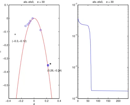
−0.4 −0.2 0 0.2 0.4

−0.5 −0.4 −0.3 −0.2 −0.1 0 0.1

(−0.3,−0.12)

(0.26,−0.34) als−els3, e = 30

d

h

0 50 100 150 200

10−6

10−5

10−4

10−3

als−els3, e = 30

Figure 1: First case treated by ALS with ELS at every 3 iterations. Left: symbols ‘+’, ‘o’ and ‘∗’ denote respectively the initial value, the successive iterations, and the global minimum, in the (d, h) plane. Right: value of the error as a function of iterations.

5.2

A

2

×

2

×

2

tensor of rank 2

Paatero gave in his paper [47] a nice example of a 2×2×2 tensor, fully parameter-izable, hence permitting reproducible experiments. We use here the same parame-terization. Its form is as follows:

T=

0 1 e 0

1 d 0 h

The discriminant defined in Section 2.2 is in the present case ∆ = 4h+d2_{e. As}

in [47], we represent the decompositions computed in the hyperplanee= 30. The

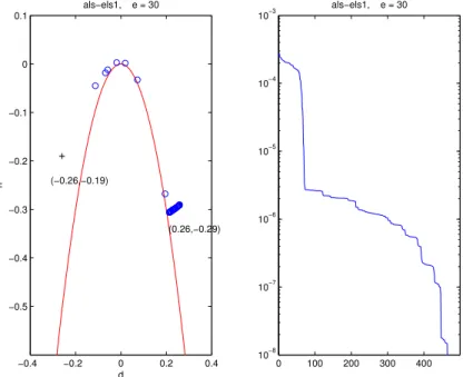
−0.4 −0.2 0 0.2 0.4 −0.5

−0.4 −0.3 −0.2 −0.1 0 0.1

(−0.26,−0.19)

(0.26,−0.29) als−els1, e = 30

d

h

0 100 200 300 400

10−8

10−7

10−6

10−5

10−4

10−3

als−els1, e = 30

Figure 2: Second case treated by ALS with ELS at every iteration. Left: symbols ‘+’, ‘o’ and ‘∗’ denote respectively the initial value, the successive iterations, and the global minimum, in the (d, h) plane. Right: value of the error as a function of iterations.

tensor to be decomposed are chosen to have a discriminant of ∆>0, so that they

have a rank 2, but they lie close to the variety ∆ = 0, represented by a parabola in the subsequent figures.

Case 1. First consider the tensor defined by (e, d, h) = (30,0.26,−0.34), and start with the initial value (e, d, h) = (30,−0.3,−0.12). In that case, neither the Gradient nor even LM converge towards the solution, and are stuck on the left side of the parabola. The ALS algorithm does not seem to converge, or perhaps does after a very large number of iterations. With the ELS enhancement executed every 3 iterations, ALS2 converges to a neighborhood of the solution (error of 10−6_{) within}

only 60 iterations, as shown in Figure 1. Then, the algorithm is slowed down for a long time before converging eventually to the solution; the beginning of this plateau

may be seen in the right graph of Figure 1. Note that itdoes not correspond to a

plateau of the objective function. In this particular example, the gain brought by ELS is very significant at the beginning. On the other hand, no gain is brought at the end of the trajectory towards the goal, where ELS cannot improve ALS2 because the directions given by ALS2 are repeatedly bad.

Case 2. Consider now a second (easier) case given by (e, d, h) = (30,0.26,−0.29), with the initial value (e, d, h) = (30,−0.26,−0.19). This time, the LM algorithm is

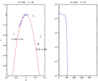
−0.4 −0.2 0 0.2 0.4 −0.5

−0.4 −0.3 −0.2 −0.1 0 0.1

(−0.26,−0.19)

(0.26,−0.29) lm−els0, e = 30

d

h

0 100 200 300 400

10−8

10−7

10−6

10−5

10−4

10−3

lm−els0, e = 30

Figure 3: Second case treated by LM. Left: symbols ‘+’, ‘o’ and ‘∗’ denote respectively the initial value, the successive iterations, and the global minimum, in the (d, h) plane. Right: value of the error as a function of iterations.

the most efficient and converges within 100 iterations, as shown in Figure 3. The fastest ALS2 algorithm is this time the one using the ELS enhancement at every iteration, and converges within 400 iterations (cf. Figure 2).

In the second case, ALS2 with the ELS enhancement could avoid being trapped in a kind of “cycling” about the goal, whereas it could not do it in the first example. This is a limitation of ELS: if the directions provided by the algorithm are bad, ELS cannot improve much on the convergence. The same has been be observed with case 1: ELS does not improve LM since directions chosen by LM are bad (LM is not represented for case 1). The other observation one can make is that executing ELS at every iteration is not always better than at everypiterations,p >1: this depends on the trajectory, and there is unfortunately no general rule. This will be also confirmed by the next computer experiments.

5.3

Random

30

×

30

×

30

tensor of rank 20

In the previous section, the computational complexity per iteration was not an issue, because it is so small. Now we shall turn our attention to this issue, with a

particular focus on the effect ofdimension reduction by HOSVD truncation. As in

the 2×2×2 case, the initial value has an influence on convergence; one initial point is chosen randomly, the same for all algorithms to be compared.

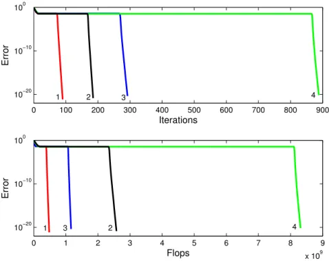
0 1 2 3 4 5 6 7 8 9 x 109 10−20

10−10 100

Flops

Error

0 100 200 300 400 500 600 700 800 900 10−20

10−10 100

Iterations

Error

4

4 3

2 1

1 3 2

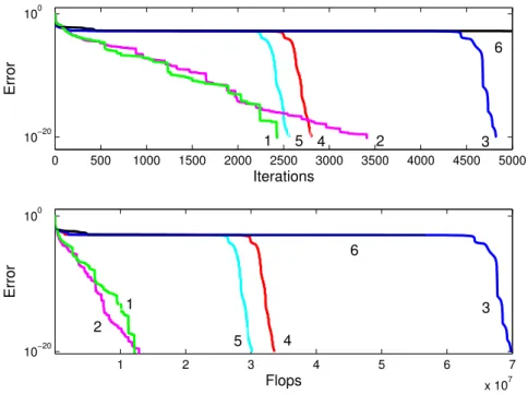
Figure 4: Reconstruction error of a 30×30×30 random tensor of rank 20 as a function of the number of iterations (top) or the number of multiplications (bottom), and for various algorithms. 1: ALS + HOSVD + ELS, 2: ALS + ELS, 3: ALS + HOSVD, 4: ALS.

The tensor considered here is generated by three 30×20 factor matrices whose

entries have been independently randomly drawn according to a zero-mean unit variance Gaussian distribution. In the sequel, we shall denote such a random draw-ing asA∼ N30×20(0,1), in short. The correlation coefficient (absolute value of the

cosine) between any pair of columns of these matrices was always smaller than 0.8, which is a way to check out that the goal to reach does not lie itself in a strong bottleneck.

The ALS algorithm is run either without ELS, or with ELS enhancement at every iteration. Figure 4 shows the clear improvement brought by ELS without dimension reduction (the computational complexity is 3 times smaller). If the dimensions are reduced to 20 by HOSVD truncation, we also observe a similar improvement: ALS runs better, but the additional complexity of ELS also becomes smaller (the rank is of same order as dimensions). Also notice by comparing top and bottom of Figure 4 that curves 2 and 3 do not appear in the same order: the dimension reduction gives the advantage to ALS in dimension 20 without ELS, compared to ALS with ELS in dimension 30. The advantage was reversed in the top part of the figure.

A reduction of the dimensions to a value smaller than 20, while keeping the rank equal to 20, is theoretically possible. However, we know that truncating the

HOSVD is not the optimal way of finding the best (20,20,20) multilinear rank

approximation. In practice, we have observed that truncating the HOSVD yields reconstruction errors if the chosen dimension is smaller than the rank (e.g. 19 in the present case or smaller).

5.4

Random

5

×

5

×

5

tensor of rank 4

The goal here is to show the interest of ELS, not only for ALS, but also for the Gra-dient algorithm. In fact in simple cases, the GraGra-dient algorithm may be attractive, if it is assisted by the ELS enhancement.

0 500 1000 1500 2000 2500 3000 3500 4000 4500 5000 10−20

100

Iterations

Error

1 2 3 4 5 6 7

x 107 10−20

100

Flops

Error

1 5 4 2 3

6

6

1 2

3

4 5

Figure 5: Reconstruction error of a 5×5×5 tensor of rank 4 as a function of the number of iterations (top) or the number of multiplications (bottom), and for various algorithms. 1: Gradient + ELS with period 2, 2: Gradient + ELS with period 5, 3: ALS + ELS with period 1 (every iteration), 4: ALS + ELS with period 5, 5: ALS + ELS with period 7, 6: ALS.

We consider the easy case of a 5×5×5 tensor of rank 4. The latter has

been built from three 5×4 Gaussian matrices drawn randomly as before, each

N5×4(0,1). Results are reported in figure 5, and show that ELS performs similarly

if executed every 2 iterations, or every 5. Results of the Gradient without ELS

enhancement are not shown, but are as poor as ALS. Convergence of the Gradient with ELS is reached earlier than ALS with ELS, but this is not always the case in general. The Gradient with ELS appears to be especially attractive in this example if computational complexity is considered.

5.5

Double bottleneck in a

30

×

30

×

30

tensor

Now more difficult cases are addressed, and we consider a tensor with two dou-ble bottlenecks (with R. Harshman terminology). The tensor is built from three

Gaussian matricesA,BandCof size 30×4, and we have created two bottlenecks

in the two first modes as follows. The first column a(1) of A is drawn randomly

as N30(0,1). Then the second column is set to be a(2) = a(1) + 0.5v(2), where

v(2) ∼ N30(0,1). The third and fourth columns of A are generated in the same

manner, that is,a(4) =a(3)+0.5v(4), wherea(3)∼ N30(0,1) andv(4)∼ N30(0,1).

MatrixB is independently generated exactly in the same manner. Vectors

belong-ing to a bottleneck generated this way have a correlation coefficient of 0.89. On the other hand, matrix C is independently N30×4(0,1), and its columns are not close

to dependent.

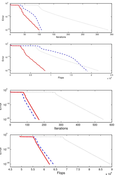
Results reported in Figure 6 show that even when the rank is moderate compared to dimensions, ELS brings improvements to ALS, despite the fact that its additional complexity is not negligible according to Equation (9). Surprisingly, a dimension reduction down to the rank value does not change this conclusion. As previously, ELS with period 1 cannot be claimed to be always better than ELS with period

p >1.

ALS with ELS enhancement at every 5 iterations (solid line in Figure 7) benefits from an important computational complexity improvement thanks to the dimension reduction down to 4: its convergences needs 6.106_{multiplications instead of 8.10}8_.

The improvement is even more impressive for ALS with ELS enhancement at every iteration (dashed line).

5.6

Swamp in a

30

×

30

×

30

tensor of rank 4

In this last example, we have generated a tensor with two triple bottlenecks, that is, a tensor that lies in a swamp. MatricesAandBare generated as in Section 5.5,

but matrixC is now also generated the same way.

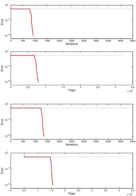
This tensor is difficult to decompose, and ALS does not converge after 5000 iterations. With the help of ELS every 5 iterations, the algorithm converges with about a thousand of iterations. This was unexpected since ELS is not always able to escape from swamps. The reduction of dimensions to 4 allows to decrease the computational complexity by a factor of 50, even if the number of iterations has slightly increased.

6

Conclusion

Our paper was three-fold. Firstly we have surveyed theoretical results, and pointed out which are still conjectures. Secondly we have described several numerical algo-rithms and given their approximate complexities for large dimensions. Thirdly, we have compared these algorithms in situations that Richard Harshman had classi-fied, and in particularmultiple bottlenecks andswamps. Several conclusions can be drawn.

First, one can claim that dimension reduction by HOSVD truncation is always improving the results, both in terms of speed of convergence and computational complexity, provided the new dimensions are not smaller than the rank of the tensor to be decomposed.

Second, ELS has been shown to be useful to improve ALS2 or the Gradient de-scent, either as an help to escape from a local minimum or to speed up convergence. ELS has been often efficient in simple or multiple bottlenecks, and even in swamps. Its help ranges from excellent to moderate. On the other hand, ELS has never been able to help LM when it was stuck.

Third, ALS2 can still progress very slowly in some cases where the objective function is not flat at all. This is a particularity of ALS, and we suspect that it is “cycling”. In such a case, ELS does not help because the directions defined by ALS2 are not good. One possibility would be to call for ALS1 to give other directions; this is currently being investigated.

Last, no solution has been proposed in cases of CP-degeneracies. In the later case, the problem is ill-posed, and the solution should be searched for by changing the modeling, i.e., either by increasing the rank or by imposing additional constraints that will avoid factor cancellations. Future works will be focussed on the two latter conclusions.

Acknowledgment. This work has been partly supported by contract ANR-06-BLAN-0074 “Decotes”.

References

[1] H. ABO, G. OTTAVIANI, and C. PETERSON. Induction for secant varieties

of Segre varieties, August 2006. arXiv:math/0607191.

[2] J. ALEXANDER and A. HIRSCHOWITZ. La methode d’Horace eclatee: ap-plication a l’interpolation en degre quatre.Invent. Math., 107(3):585–602, 1992.

[3] D. BINI. Border rank of a p×q×2 tensor and the optimal approximation

of a pair of bilinear forms. In Proc. 7th Col. Automata, Languages and

Pro-gramming, pages 98–108, London, UK, 1980. Springer-Verlag. Lecture Notes in Comput. Sci., vol. 85.

[4] D. BINI. Border rank of m×n×(mn−q) tensors. Linear Algebra Appl.,

79:45–51, 1986.

[5] M. C. BRAMBILLA and G. OTTAVIANI. On the Alexander-Hirschowitz

the-orem. Jour. Pure Applied Algebra, 212:1229–1251, 2008.

[6] R. BRO. Parafac, tutorial and applications.Chemom. Intel. Lab. Syst., 38:149– 171, 1997.

[7] R. BRO and C. A. ANDERSSON. Improving the speed of multiway algorithms.

part ii: Compression. Chemometrics and Intelligent Laboratory Systems,

42(1-2):105–113, 1998.

[8] P. B ¨URGISSER, M. CLAUSEN, and M. A. SHOKROLLAHI. Algebraic

Com-plexity Theory, volume 315. Springer, 1997.

[9] J. D. CARROLL and J. J. CHANG. Analysis of individual differences in mul-tidimensional scaling via n-way generalization of Eckart-Young decomposition.

Psychometrika, 35(3):283–319, September 1970.

[10] A. CAYLEY. On the theory of linear transformation. Cambridge Math. J.,

4:193–209, 1845.

[11] T. F. CHAN. An improved algorithm for computing the singular value

decom-position. ACM Trans. on Math. Soft., 8(1):72–83, March 1982.

[12] L. CHIANTINI and C. CILIBERTO. On the concept ofk−sectant order of a

variety. J. London Math. Soc., 73(2), 2006.

[13] P. COMON. Tensor decompositions. In J. G. McWhirter and I. K. Proudler,

editors, Mathematics in Signal Processing V, pages 1–24. Clarendon Press,

Oxford, UK, 2002.

[14] P. COMON, G. GOLUB, L-H. LIM, and B. MOURRAIN. Symmetric

ten-sors and symmetric tensor rank. SIAM Journal on Matrix Analysis Appl.,

30(3):1254–1279, 2008.

[15] P. COMON and G. H. GOLUB. Tracking of a few extreme singular values and vectors in signal processing.Proceedings of the IEEE, 78(8):1327–1343, August 1990. (published from Stanford report 78NA-89-01, feb 1989).

[16] P. COMON and B. MOURRAIN. Decomposition of quantics in sums of powers

of linear forms. Signal Processing, Elsevier, 53(2):93–107, September 1996.

special issue on High-Order Statistics.

[17] P. COMON and M. RAJIH. Blind identification of under-determined mix-tures based on the characteristic function. Signal Processing, 86(9):2271–2281, September 2006.

[18] P. COMON and J. ten BERGE. Generic and typical ranks of three-way arrays. InIcassp’08, Las Vegas, March 30 - April 4 2008.

[19] P. COMON, J. M. F. ten BERGE, L. DeLATHAUWER, and J. CASTAING.

Generic and typical ranks of multi-way arrays. Linear Algebra Appl., 2008.

submitted.

[20] D. COX, J. LITTLE, and D. O’SHEA. Ideals, Varieties, and Algorithms: An

Introduction to Computational Algebraic Geometry and Commutative Algebra. Undergraduate Texts in Mathematics. Springer Verlag, New York, 1992. 2nd ed. in 1996.

[21] A. L. F. de ALMEIDA, G. FAVIER, and J. C. M. MOTA. PARAFAC-based unified tensor modeling for wireless communication systems with application to blind multiuser equalization. Signal Processing, 87(2):337–351, February 2007.

[22] L. DeLATHAUWER. A link between canonical decomposition in multilinear

algebra and simultaneous matrix diagonalization. SIAM Journal on Matrix

Analysis, 28(3):642–666, 2006.

[23] L. DeLATHAUWER and J. CASTAING. Tensor-based techniques for the blind

separation of DS-CDMA signals. Signal Processing, 87(2):322–336, February

2007.

[24] L. DeLATHAUWER, B. de MOOR, and J. VANDEWALLE. A multilinear

singular value decomposition. SIAM Jour. Matrix Ana. Appl., 21(4):1253–

1278, April 2000.

[25] L. DeLATHAUWER, B. de MOOR, and J. VANDEWALLE. On the best

rank-1 and rank-(R1,R2,...RN) approximation of high-order tensors. SIAM

Jour. Matrix Ana. Appl., 21(4):1324–1342, April 2000.

[26] R. EHRENBORG. Canonical forms of two by two matrices. Jour. of Algebra,

213:195–224, 1999.

[27] G. H. GOLUB and C. F. VAN LOAN. Matrix computations. Hopkins Univ.

Press, 1989.

[28] G. H. GOLUB and V. PEREYRA. Differentiation of pseudo-inverses, separable nonlinear least square problems and other tales. In M. Z. Nashed, editor,

Generalized Inverses and Applications, pages 303–324. Academic Press, New York, 1976.

[29] R. A. HARSHMAN. Foundations of the Parafac procedure: Models and

con-ditions for an explanatory multimodal factor analysis. UCLA Working Papers

in Phonetics, 16:1–84, 1970. http://publish.uwo.ca/ harshman.

[30] R. A. HARSHMAN. An annoted bibliogrtaphy of articles on

degenerate solutions or decompositions, 2004. Unpublished,

http://publish.uwo.ca/∼harshman/bibdegen.pdf.

[31] R. A. HARSHMAN and M. E. LUNDY. Parafac: Parallel factor analysis.

Computational Statistics and Data Analysis, pages 39–72, 1994.

[32] F. L. HITCHCOCK. Multiple invariants and generalized rank of a p-way matrix or tensor. J. Math. and Phys., 7(1):39–79, 1927.

[33] W. P. KRIJNEN, T. K. DIJKSTRA, and A. STEGEMAN. On the non-existence of optimal solutions and the occurrence of degeneracy in the

Can-decomp/Parafac model. Psychometrika, 73(3):431–439, September 2008.

[34] P. KROONENBERG.Three mode Principal Component Analysis. SWO Press,

Leiden, 1983.

[35] J. B. KRUSKAL. Three-way arrays: Rank and uniqueness of trilinear

decom-positions. Linear Algebra and Applications, 18:95–138, 1977.

[36] J. B. KRUSKAL, R. A. HARSHMAN, and M. E. LUNDY. How 3-MFA data can cause degenerate Parafac solutions, among other relationships. In R. Coppi

and S. Bolasco, editors,Multiway Data Analysis, pages 115–121. Elsevier

Sci-ence, North-Holland, 1989.

[37] J. M. LANDSBERG. Kruskal’s theorem, 2008. private communication.

[38] E. LASKER. Kanonische formen. Mathematische Annalen, 58:434–440, 1904.

[39] T. LICKTEIG. Typical tensorial rank. Linear Algebra Appl., 69:95–120, 1985.

[40] L-H. LIM and P. COMON. Nonnegative approximations of nonnegative tensors.

J. Chemometrics, 2008. this issue.

[41] K. MADSEN, H. B. NIELSEN, and O. TINGLEFF. Methods for Non-Linear

Least Squares Problems. Informatics and mathematical Modelling. Technical University of Denmark, 2004.

[42] M. MELLA. Singularities of linear systems and the Waring problem. Trans.

Am. Math. Soc., 358(12), December 2006.

[43] B. C. MITCHELL and D. S. BURDICK. Slowly converging Parafac sequences:

Swamps and two-factor degeneracies. Jour. Chemometrics, 8:155–168, 1994.

[44] C. NAVASCA, L. De LATHAUWER, and S. KINDERMANN. Swamp

reduc-ing technique for tensor decomposition. In 16th European Signal Processing

Conference (Eusipco’08), Lausanne, August 25-29 2008.

[45] D. NION and L. DeLATHAUWER. An enhanced line search scheme for

complex-valued tensor decompositions. application in DS-CDMA. Signal

Pro-cessing, 88(3):749755, March 2008.

[46] P. PAATERO. The multilinear engine: A table-driven, least squares program for solving multilinear problems, including the n-way parallel factor analysis

model. Journal of Computational and Graphical Statistics, 8(4):854–888,

De-cember 1999.

[47] P. PAATERO. Construction and analysis of degenerate Parafac models. Jour. Chemometrics, 14:285–299, 2000.

[48] M. RAJIH and P. COMON. Enhanced line search: A novel method to accel-erate Parafac. InEusipco’05, Antalya, Turkey, Sept. 4-8 2005.

[49] M. RAJIH, P. COMON, and R. HARSHMAN. Enhanced line search : A novel

method to accelerate PARAFAC. SIAM Journal on Matrix Analysis Appl.,

30(3):1148–1171, September 2008.

[50] C. R. RAO. Linear Statistical Inference and its Applications. Probability and

Statistics. Wiley, 1965.

[51] C.R. RAO and S. MITRA. Generalized Inverse of Matrices and Its

Applica-tions. New York: Wiley, 1971.

[52] W. S. RAYENS and B. C. MITCHELL. Two-factor degeneracies and a stabi-lization of Parafac. Chemometrics Intell. Lab. Syst., 38:173–181, 1997.

[53] J. RISSANEN.Stochastic Complexity in Statistical Inquiry, volume 15 ofSeries in Computer Science. World Scientific Publ., London, 1989.

[54] N. D. SIDIROPOULOS and R. BRO. On the uniqueness of multilinear

decom-position of N-way arrays. Jour. Chemo., 14:229–239, 2000.

[55] N. D. SIDIROPOULOS, G. B. GIANNAKIS, and R. BRO. Blind PARAFAC

receivers for DS-CDMA systems. Trans. on Sig. Proc., 48(3):810–823, March

2000.

[56] V. De SILVA and L-H. LIM. Tensor rank and the ill-posedness of the best

low-rank approximation problem. SIAM Journal on Matrix Analysis Appl.,

30(3):1084–1127, 2008.

[57] A. SMILDE, R. BRO, and P. GELADI. Multi-Way Analysis. Wiley, 2004.

[58] A. STEGEMAN. Degeneracy in Candecomp/Parafac explained forp×p×2

arrays of rankp+ 1 or higher. Psychometrika, 71(3):483–501, 2006.

[59] A. STEGEMAN. Degeneracy in Candecomp/Parafac and Indscal explained for several three-sliced arrays with a two-valued typical rank. Psychometrika, 72(4):601–619, 2007.

[60] A. STEGEMAN. Low-rank approximation of generic pxqx2 arrays and

diverg-ing components in the Candecomp/Parafac model. SIAM Journal on Matrix

Analysis Appl., 30(3):988–1007, 2008.

[61] A. STEGEMAN and N. D. SIDIROPOULOS. On Kruskal’s uniqueness

con-dition for the Candecomp/Parafac decomposition. Linear Algebra and Appl.,

420:540–552, 2007.

[62] V. STRASSEN. Rank and optimal computation of generic tensors. Linear Algebra Appl., 52:645–685, July 1983.

[63] J. M. F. ten BERGE. Kruskal’s polynomial for 2×2×2 arrays and a

general-ization to 2×n×narrays. Psychometrika, 56:631–636, 1991.

[64] J. M. F. ten BERGE. The typical rank of tall three-way arrays.Psychometrika,

65(5):525–532, September 2000.

[65] J. M. F. ten BERGE. Partial uniqueness in CANDECOMP/PARAFAC. Jour.

Chemometrics, 18:12–16, 2004.

[66] J. M. F. ten BERGE and H. A. L. KIERS. Simplicity of core arrays in

three-way principal component analysis and the typical rank of pxqx2 arrays.Linear

Algebra Appl., 294:169–179, 1999.

[67] J. M. F. ten BERGE and A. STEGEMAN. Symmetry transformations for square sliced three way arrays, with applications to their typical rank. Linear Algebra Appl., 418:215–224, 2006.

[68] A. TERRACINI. Sulla rappresentazione delle forme quaternarie mediante

somme di potenze di forme lineari. Atti della R. Acc. delle Scienze di Torino, 51, 1916.

[69] G. TOMASI and R. BRO. A comparison of algorithms for tting the Parafac

model. Comp. Stat. Data Anal., 50:1700–1734, 2006.

[70] L. R. TUCKER. Some mathematical notes for three-mode factor analysis.

Psychometrika, 31:279–311, 1966.

0 50 100 150 200 250 300 350

10−20

10−10

100

Iterations

Error

0 0.5 1 1.5 2 2.5

x 108

10−20

10−10

100

Flops

Error

0 100 200 300 400 500 600 10−20

10−10 100

Iterations

Error

4.5 5 5.5 6 6.5 7 7.5 8 8.5 9 x 106 10−20

10−10 100

Flops

Error

Figure 6: Reconstruction error of a 30×30×30 tensor of rank 4 with 2 double bottlenecks as a function of the number of iterations or the number of multiplications, and for various algorithms. Solid: ALS + ELS with period 5, dashed: ALS + ELS with period 1 (at every iteration), dotted: ALS. Top: without dimension reduction, bottom: after reducing dimensions down to to 4.

0 500 1000 1500 2000 2500 3000 3500 4000 4500 5000

10−20

10−10

100

Iterations

Error

0 0.5 1 1.5 2 2.5 3 3.5

x 109

10−20

10−10

100

Flops

Error

0 500 1000 1500 2000 2500 3000 3500 4000 4500 5000

10−20

10−10

100

Iterations

Error

0 0.5 1 1.5 2 2.5 3 3.5 4 4.5

x 107

10−20

10−10

100

Flops

Error

Figure 7: Reconstruction error of a 30×30×30 of rank 4 with 2 triple bottlenecks as a function of the number of iterations (top) or the number of multiplications (bottom), and for various algorithms. Solid: ALS + ELS with period 5, dotted: ALS. Top: without dimension reduction, bottom: after reducing dimensions down to to 4.