Cooperative navigation of multiple Marine Robotic Vehicles

F

E

U

P

Cooperative navigation of multiple

Marine Robotic Vehicles

Nuno Alberto Moreira Maia

Mestrado Integrado em Engenharia Eletrotécnica e de Computadores Supervisor: António Pedro Aguiar

Resumo

Com a constante evolução da navegação e exploração, a humanidade sempre quis alcançar mais e elevar o conhecimento humano acerca do mundo para além dos seus limites. Tendo explorado cada continente, muito há ainda por descobrir no fundo dos oceanos. Devido a custos monetários e a ser pouco viável no que diz respeito a dispendiosos recursos humanos, a exploração de ambientes subaquáticos é feita através da utilização de veículos robóticos autónomos. Esta possibilidade não só é mais segura, não colocando em risco vidas humanas em territórios inóspitos, mas também é, em alguns aspectos, mais fácil de implementar. Como estes veículos são não tripulados, eles precisam de ser autónomos e vigiados à distância. Isto levou à importância do desenvolvimento de técnicas de navegação.

Em terra, esta navegação é possível através do sistema de posicionamento já bem conhecido, GPS. No entanto, debaixo de água é impossível usar este sistema devido ao facto de esses sinais não se propagarem bem neste meio. Há a necessidade de utilizar outro tipo de sinais, que neste momento são ondas acústicas pois se propagam bem nesse meio. Para calcular a localização do veículo subaquático, a ideia principal é usar o sistema de emissores/receptores que enviam e re-cebem do veículo o sinal acústico. Através da medida do tempo de viagem e sabendo a velocidade do sinal acústico, é então possível encontrar a localização do objecto. Em 2D (ou seja, sabendo a profundidade) só são necessários três emissores/receptores (assumindo certas condições espaci-ais) para descobrir a localização: um dá uma circunferência de possíveis localizações, dois dão duas circunferências interceptadas em dois pontos, o que significa duas localizações possíveis, e o terceiro intercepta uma destas localizações, que é a localização correta do veículo, este processo é designado trilateração. No entanto, o vasto número de emissores/receptores que são usados é dispendioso, sentindo-se a necessidade de encontrar uma maneira de calcular a localização de veículos utilizando menos emissores/receptores.

Com a utilização de apenas um emissor/receptor e implementando um algoritmo que calcula o deslocamento do veículo em diferentes tempos, é possível criar uma rede virtual de emissores/re-ceptores que vai ajudar a encontrar uma estimativa da posição do veículo. Esta estimativa da localização é mais tarde filtrada usando o filtro de Kalman. O papel deste filtro é, não só filtrar o ruido, mas também complementar o resultado da trilateraçao com informação da velocidade linear relativa obtida por um doppler e para lidar com possíveis perturbações desconhecidas tais como as correntes. De facto, testes foram feitos e mostraram que sem a utilização do filtro de Kalman e sob a influência destas correntes, o algoritmo utilizado diverge, não dando os resultados pretendidos.

Depois de ter o algoritmo de navegação implementado para um veículo, mais uma camada de complexidade foi adicionada ao incluir outro veículo com o papel de emissor/receptor (emis-sor/receptor com movimento) no sentido de tornar a navegação cooperativa. O veículo que fun-ciona como emissor/receptor para outros veículos pode ser um veículo robótico de superfície e por isso, deste modo, ser capaz de utilizar o sistema GPS. Pode também ser um veículo submarino robótico autónomo que serve de emissor/receptor a outros e dos quais a sua posição também pode ser calculada usando uma lógica semelhante à utilizada na navegação singular.

Abstract

With the increased evolution in navigation and exploration, mankind always aimed to go further and push the human knowledge of the world to its limits. Having explored every continent and land surface, much is still left to be discovered underneath the oceans. Due to monetary costs and not being viable due to being too costly in human resources, the exploration of underwater territories is being carried out through the use of autonomous robotic vehicles. This possibility not only is safer, not endangering human lives in inhospitable locations, but it also is in some aspects easier to implement. As these vehicles are unmanned, they need to be autonomous and surveyed from a distance. This led to the importance of the development of navigation techniques.

On land, this navigation is possible through the well-known GPS system. However, underwa-ter it is impossible to use this system due to the fact that those signals do not propagate well in such an environment. There is the need to use another type of signals, which presently turns out to be acoustic waves since these signals propagate well in this environment.

To compute the location of an underwater vehicle, the main idea is to use a system of transpon-ders/beacons that send to and receive from the vehicle an acoustic signal. By measuring the time of travel and knowing the speed of the underwater acoustic signal (AS) it is then possible to find the location of the object. In 2D, (which means knowing the depth) it only takes three beacons (under some spatial assumptions) to find out the location: one gives a circumference of possible locations, two give 2 circumferences which are intercepted in two places, which mean two possi-ble locations and the third one intercepts one of these locations, which is the right location of the vehicle, this process is called trilateration. However, the vast amount of transponders (beacons) that are used is very costly, so there is a need to find a way to compute the location of the vehicles using fewer resources.

With the use of only one beacon, and implementing an algorithm that computes the displace-ment of the vehicle in different times, it is possible to create a virtual net of beacons which will help finding out an estimate of the vehicle location.

This estimate of the location is later filtered using a Kalman Filter (KF). The role of this filter is to not only filter out the noise, but it is also to complement the result of the trilateration with the relative linear velocity information provided by a doppler and to deal with possible unknown underwater current disturbances. In fact, tests were done that showed that without using the KF and under the influence of currents, the algorithm would diverge, not producing the results intended.

After having the Single Beacon Navigation (SBN) for one vehicle implemented, one more layer of complexity was added by including another vehicle with the role of the beacon (moving beacon) in order to make the navigation cooperative. The vehicle that works as a beacon to the other vehicles can be an Autonomous Surface Craft (ASC) which floats at the surface of the sea and therefore uses the GPS system. It can also be an Autonomous Underwater Vehicle (AUV) which serves as a beacon to others and whose position is computed using a similar logic as the one in the SBN algorithm.

Acknowledgements

An enormous thank you to my supervisor António Pedro Aguiar, for his patience, support, guid-ance, and availability, despite always having a full schedule. It was important to have a good supervisor, since I knew little about this topic and programming was never my best skill (which is why this dissertation helped me so much in improving my skills and knowledge as I knew close to nothing about what to do).

A big cheers to my father, who was my -’at home’ supervisor, helping me understand some important aspects of what I had to do and helping me think when I couldn’t find the right way alone.

I would like to thank my family for their help, not only during this semester, while I was doing the dissertation, but also for supporting my choices, even if it meant going to Romania and Brazil for six months each.

Thanks to Agostinho Rocha, André Reis and José Oliveira, for their help in some aspects I needed to learn about in order to complete this dissertation.

And finally, thanks for these great years in college, Tiago Maia, Fabio Silva, Alexandre Santos, Miguel Ribeiro, Luciano Santos, Nuno Guimarães, Bruno Pereira, and the list goes on; without a doubt these years will be missed and remembered with the willingness to go back and relive it all.

Nuno Alberto Moreira Maia

”Life begins at the end of your comfort zone.”

Neale Donald Walsch

Contents

2 State of the Art 5 2.1 Some well-known historic examples . . . 5

2.1.1 Space . . . 5

2.1.2 Land . . . 6

2.1.3 Air . . . 7

2.1.4 Ocean . . . 8

2.2 Doppler Effect . . . 9

2.3 Current Underwater Navigation Systems . . . 12

2.3.1 Long Baseline . . . 12

2.3.2 Marine robotic platforms . . . 13

2.3.3 Recent Projects . . . 18

3 Navigation for single Marine Robotic Vehicles 21 3.1 System overview . . . 21

3.2 Kinematic vehicle model . . . 22

3.3 Trilateration . . . 22

3.3.1 Forming the Virtual Net of Beacons . . . 22

3.3.2 Optimization . . . 24

3.4 Kalman Filter . . . 27

3.4.1 About the filter . . . 27

3.4.2 Kalman filter implementation in this project . . . 29

4 Cooperative Navigation 33 4.1 CN between AUV and ASC . . . 34

4.2 CN between AUV and AUV . . . 35

5 Results and discussion 37 5.1 Single Navigation . . . 37

5.1.1 Straight Line Movement . . . 38

5.1.2 Circular Movement . . . 40

5.1.3 S Movement . . . 42

5.2 Cooperative Navigation - Between ASC and AUV . . . 44 ix

5.2.1 Straight Line Movement of the ASC . . . 45

5.2.2 Circular Movement of the ASC . . . 47

5.2.3 S Movement of the ASC . . . 50

5.2.4 N Movement of the ASC . . . 52

5.3 Cooperative Navigation - Between AUV and AUV . . . 54

6 Conclusions and Further Research 55 6.1 Summary . . . 55

6.2 Further Research . . . 55

A Appendix 1 57 A.1 Schematics and schemes . . . 57

A.2 MatLab blocks and modules code . . . 59

A.3 Some more simulation results . . . 72

List of Figures

1.1 AUV fleet in underwater exploration (Source: [1] ) . . . 1

1.2 Communication between AUV, ASC and station unit (Source: htt p : //goo.gl/Qrb2t) 2 2.1 MER exploring Mars surface (Source: htt p : //goo.gl/ILOzi) . . . 6

2.2 One of the first robotic volcanoes explorers (Source: htt p : //goo.gl/8T s6A) . . 7

2.3 Aerial robot explorer (Source: htt p : //goo.gl/8e f Bh) . . . 8

2.4 Underwater robotic explorer (Source: htt p : //goo.gl/CHX rl) . . . 9

2.5 Glider (Source: htt p : //goo.gl/V lS f a) . . . 9

2.6 Doppler explanation (Source: htt p : //goo.gl/k9 f zz) . . . 10

2.7 Doppler functioning (Source: htt p : //goo.gl/627KC) . . . 11

2.8 Dropping Sonobuoy (Source: htt p : //goo.gl/uI2Nm) . . . 11

2.9 LBL (Source: htt p : //goo.gl/VV BQa) . . . 13

2.10 Position obtained using 3 beacons trilateration (Source: http://goo.gl/uiXuX) . . 13

2.11 FEUP AUV MARES (Source: htt p : //goo.gl/pxa1B) . . . 14

2.12 Light Autonomous Underwater Vehicle (Source: htt p : //goo.gl/mrX ai) . . . . 15

2.13 ASV Zarco (Source: htt p : //goo.gl/pxa1B) . . . 17

2.14 Navigation Instrumentation Buoy (Source: htt p : //goo.gl/pxa1B) . . . 18

3.1 System block diagram . . . 21

3.2 Network of beacons creation (Source: [2]) . . . 23

3.3 Optimizing a function (Source: http://goo.gl/I9Vba) . . . 25

3.4 Gradient Descent algorithm . . . 26

3.5 Newton’s Method algorithm . . . 27

3.6 Kalman filter block diagram . . . 28

3.7 Algorithm block diagram (Source: [2]) . . . 31

4.1 Cooperative navigation between ASC and AUV (Source: [1]) . . . 34

4.2 Underwater fleet navigation (Source: http://goo.gl/D9CJ4) . . . 34

5.1 Line movement without noise or current . . . 38

5.2 Line movement with noise and without current . . . 39

5.3 Line movement with current and without noise . . . 39

5.4 Line movement with current and noise . . . 40

5.5 Circular movement without current or noise . . . 40

5.6 Circular movement with noise and without current . . . 41

5.7 Circular movement with current and without noise . . . 41

5.8 Circular movement with current and noise . . . 42

5.9 S movement without current or noise . . . 43

5.10 S movement with noise and without current . . . 43 xi

5.11 S movement with current and without noise . . . 44

5.12 S movement with current and noise . . . 44

5.13 Line movement without current or noise . . . 45

5.14 Line movement with noise and without current . . . 46

5.15 Line movement with current and without noise . . . 46

5.16 Line movement with current and noise . . . 47

5.17 Circular movement without current or noise . . . 47

5.18 Circular movement with noise and without current . . . 48

5.19 Circular movement with current and without noise . . . 48

5.20 Circular movement with current and noise . . . 49

5.21 Circular movement with current and noise . . . 49

5.22 S movement without current or noise . . . 50

5.23 S movement with noise and without current . . . 50

5.24 S movement with current and without noise . . . 51

5.25 S movement with current and without noise . . . 51

5.26 S movement with current and noise . . . 52

5.27 S movement without current or noise . . . 52

5.28 S movement with noise and without current . . . 53

5.29 S movement current and without noise . . . 53

5.30 S movement with current and noise . . . 54

A.1 AUV block . . . 57

A.2 ASC Beacon . . . 57

A.3 Cooperative ASC and AUV . . . 58

A.4 Velocity main without noise . . . 72

A.5 Velocity with noise . . . 72

A.6 Velocity without noise . . . 73

A.7 Velocity with noise . . . 73

A.8 Velocity without noise . . . 73

List of Tables

2.1 Characteristics of MARES . . . 14

2.2 Characteristics of LAUV . . . 16

2.3 Characteristics of the ASVs or ASCs . . . 17

2.4 Characteristics of the Buoy . . . 18

Nomenclature

AS Acoustic Signal

ASC Autonomous Surface Craft ASV Autonomous Surface Vehicles AUV Autonomous Underwater Vehicle CN Cooperative Navigation

COTS Commercial off-the-shelf DE Doppler Effect

FEUP Faculdade de Engenharia da Universidade do Porto GDM Gradient Descent Method

GPS Global Positioning System ISR Robotic Systems Institute KF Kalman Filter

LAUV Light Autonomous Underwater Vehicle LBL Long Baseline

LSTS Underwater Systems and Technology Laboratory MARES Modular Autonomous Robot for Environment Sampling MER Mars Exploration Rover

NIBs Navigation and Instrumental Buoys NM Newtow’s Method

NP Noptilus Project OM Optimization Method RV Robotic Vehicles SB Single Beacon

SBN Single Beacon Navigation SN Single Navigation

VNB Virtual Net Beacon VB Virtual Beacon Symbols ω Angular Velocity s Seconds ν Linear Velocity xv

Chapter 1

Introduction

With the increasing number of unmanned vehicles used in hardly accessible locations in missions, reconnaissance or other exploration objectives, it began to be felt a need for cooperation between those vehicles, and in particular, the use (directly or implicitly) of the navigation sensors from the neighbour vehicles to obtain better navigation performance. The concept of navigation is the act of computing for a vehicle the evolution of its linear and rotational positions and velocities. In the underwater medium, this is a challenging task because GPS is not available. To counter this problem we will use Acoustic Signals (ASs), combined with the Doppler Effect and measure-ments provided by inertial measurement unit sensors to be able to track the underwater location of the vehicle. After the navigation problem is sorted out we can start implementing cooperative behaviour (Figure 1.1) in the vehicles, such as location feedback, formation abilities and many other possibilities are unlocked.

Figure 1.1: AUV fleet in underwater exploration (Source: [1] )

1.1

Motivation

Underwater navigation is a critical and difficult task (Fig. 1.2). In this thesis we propose a naviga-tion algorithm for AUVs that relies on single beacon acoustic naviganaviga-tion techniques and takes into account the presence of unknown ocean currents. This idea has advantages compared to the usual method implemented that uses three beacons since relying on multiple beacons means the need to survey more locations, and the deploy, survey and recovery of these beacons,which is costly and time expensive. After implementing the SNB approach it is then possible to make the navigation cooperative which enables a set of different abilities for the group of vehicles.

Figure 1.2: Communication between AUV, ASC and station unit (Source: htt p : //goo.gl/Qrb2t)

1.2

Objectives

The main objective of this work was to to study, develop and implement cooperative navigation algorithms for marine vehicles. In particular, the following tasks were addressed:

• Literature review and study of estimation algorithms for navigation.

• Study and implementation in Matlab of a single beacon acoustic navigation algorithm. • Study and design of cooperative estimation strategies for navigation of multiple autonomous

Robotic Vehicles (RVs).

• Implementation and evaluation of the algorithms developed through computer simulations.

1.3

Main contribution

1.4 Thesis Outline 3

• Implementation and performance evaluation through computer simulations of a single bea-con navigation algorithm for single AUVs based on the work of [2]. The algorithm is posed by two main components: the construction of net of virtual beacons and the com-putation of a first rough position through trilateration, and second a fine estimation of the position using a Kalman filter.

• The extension of the single navigation system to cooperative navigation where in this case we have at least one vehicle playing the role of a moving beacon (contrary to the first case where the beacon is stationary) serving other vehicles for navigation that interact with it.

1.4

Thesis Outline

The remainder of this dissertation is organized as follows:

• Chapter 2 describes the State of the Art starting with a brief historical explanation as well as the present technologies of this topic.

• Chapter 3 presents the implementation of the SBN.

• Chapter 4 describes the extension of the SB algorithm to multiple vehicles using a coop-erative strategy. Two cases are studied in detail: CN with AUV/ASC and CN with two AUVs.

• Chapter 5 presents the results and the critical analysis of the algorithm simulations.

• Chapter 6 concludes this thesis with a summary of the results obtained and benefits and drawbacks of the methods proposed, and suggests directions for future investigation.

Chapter 2

State of the Art

2.1

Some well-known historic examples

Throughout the history of exploration and navigation, there are some marks that are worth men-tioning. Without a doubt, exploration has been in the eager mind of mankind all along. At first, even though the navigation and the positioning systems of the time were not very precise or so-phisticated, the need to travel beyond the unknown pushed us through the oceans and, continent after continent, zone after zone, the knowledge of the entire planet started adding up and fitting in like pieces of a puzzle. We can say that this helped greatly in technological progress, not only due to the instruments that were invented to make travelling possible and finding the way people wanted to travel; but also by making the world more united and enabling the findings of each country, zone, place available everywhere.

2.1.1 Space

The most recent and remarkable event of exploration and navigation is the Mars Exploration Rover Mission (MER) conducted by NASA, which consisted in sending two rovers, Spirit (MER-A) and Opportunity (MER-B) to explore Mars’ surface and geology. See Figure 2.1. Basically, the goal of this mission is research related to the past existence of water activity (always mankind’s number one goal because it is intimately related to life and the possibility of Mars being a future place for people to live in). This project is a very costly investment in exploration, summing up to several hundreds of million dollars.

Figure 2.1: MER exploring Mars surface (Source: htt p : //goo.gl/ILOzi)

2.1.2 Land

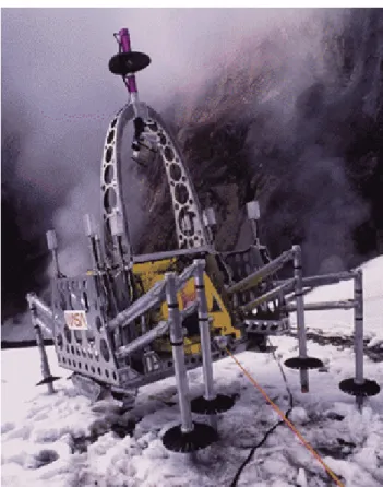
Robots are used to explore places that are dangerous to man. An example of this are the robots used to explore volcanoes and big, deep caves that are at risk of collapsing. Many projects are currently under development for monitoring volcanic activity, which would otherwise be close to impossible. See Figure 2.2. They are used to make crucial observations and taking measures which can determine the future activity of the volcanoes, knowledge that can therefore save more lives in the future. These kinds of robots have got a wide set of tools which help in making eruption scouting possible, such as ways to collect samples, sensors for data acquisition and such. The very first robotic prototypes were used in this field, and after scientists saw their success and potential, the idea of exploring other planets in a similar way, with the improvement of technology, came to mind. [3]

Another more recent example used in volcano exploration is the Robovolc, a versatile robot with more mobility and independence than its counterpart, with a better set of tools and which does not rely as much on other devices and works wireless. [4]

2.1 Some well-known historic examples 7

Figure 2.2: One of the first robotic volcanoes explorers (Source: htt p : //goo.gl/8T s6A)

2.1.3 Air

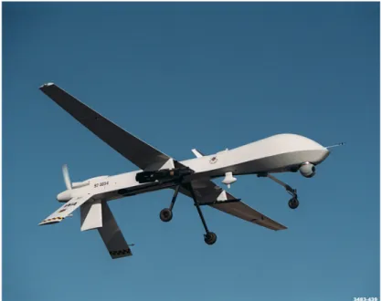
There is also a very important use for air vehicles, in robotic navigation. For instance, there are some tasks that regularly require the use of unmanned aerial vehicles. For example, they are used for ground surveillance, space reconnaissance, to find people in rescue operations and to monitor traffic. See Figure 2.3. For such operations it is common to use not single unmanned vehicles but fleets, which do CN with one another. This kind of navigation enables formation flight that is very useful for scouting wider areas and allows air-refuelling. [5]

Figure 2.3: Aerial robot explorer (Source: htt p : //goo.gl/8e f Bh)

2.1.4 Ocean

The ocean is still an environment that is very unknown to man. Covering the vast majority of the Earth, only a very small portion of it has already been scouted. Due to their inhospitable nature, it was not possible to explore deep seas up until recently. Shallow locations can be explored by humans, but the majority of the ocean is very deep and cannot be explored by divers. Even manned vehicles are inferior to RVs when it comes to ocean exploration. In this case, robotic exploration became a quick reality. Considering the fact that the deepest oceans potentially keep some of life’s most important secrets, this field is bound to be very popular in the future of exploration. See Figure 2.4. Some vehicles called gliders are used to collect data from the oceans being able to cover distances up to 600 km and representing a large contribution to future research concerning these environments. See Figure 2.5. [6] [7]

2.2 Doppler Effect 9

Figure 2.4: Underwater robotic explorer (Source: htt p : //goo.gl/CHX rl)

Figure 2.5: Glider (Source: htt p : //goo.gl/V lS f a)

2.2

Doppler Effect

As any object moves through the fluid, the fluid near the object is disturbed. The disturbances are transmitted through the fluid at a distinct speed called the speed of sound. See Figure 2.6.

As explained by NASA, sound moves through the fluid as a series of waves. The distance between any two waves is called the wavelength and the time interval between waves passing is called the period. The wavelength and the frequency are related by the speed of sound; high frequency implies short wavelength and low frequency implies a long wavelength. Shorter wave-lengths produce higher pitches. In an ideal fluid, the speed of transmission of the sound remains a constant regardless of the frequency or the wavelength. The speed of sound only depends on the state of the fluid (or gas) not on the characteristics of the generating source. [8]

They say that, because the speed of sound depends only on the state of the gas, some interesting physical phenomena occurs when a sound source moves through a uniform gas. As the source moves it continues to generate sound waves which move at the speed of sound. Since the source is moving slower than the speed of sound, the waves move out away from the source. Upstream (in the direction of the motion), the waves bunch up and the wavelength decreases. Downstream, the waves spread out and the wavelength increases. The sound that our ear detects will change in pitch as the object passes. This change in pitch is called a Doppler Effect (DE). There are equations that describe the DE. For example in the air, as the moving source approaches our ear, the wavelength is shorter, the frequency is higher and we hear a higher pitch. If we call the approaching frequency fa, the speed of sound a, the velocity of the approaching source u, and the frequency of the sound at the source f , then

fa= f a

a− u (2.1)

Figure 2.6: Doppler explanation (Source: htt p : //goo.gl/k9 f zz)

Putting it simply: the DE is the change in frequency of a wave, from an observer moving relative to its source. This happens as the source of the waves is moving toward the observer. For instance, every wave crest is emitted from a closer range, arriving quicker, therefore reducing the time between waves and increasing its frequency. See Figure 2.7.

2.2 Doppler Effect 11

Figure 2.7: Doppler functioning (Source: htt p : //goo.gl/627KC)

Depending on the medium in which they propagate, the velocity of the source and observer varies. [9]

The DE can result from • Motion of the source; • Motion of the observer; • Motion of the medium.

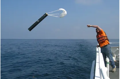
In our case, underwater vehicles, the Doppler Shift of a target is used to determine the speed of a submarine using both passive and active sonar systems. See Figure 2.8. As a submarine passes by a passive sonobuoy, the stable frequencies undergo a Doppler shift, and the speed and range from the sonobuoy can be calculated. If the sonar system is mounted on a moving ship or another submarine, then the relative velocity can be calculated.

2.3

Current Underwater Navigation Systems

Nowadays, underwater navigation is a complex concept that involves many variables.

As explained, acoustic waves, resulting from vibration in water particles, are used for naviga-tion and communicanaviga-tion between vehicles.

AUVs are equipped with an omni-directional transducer which is capable of sending and re-ceiving acoustic signals, managing to locate its position. The AUV sends signals to beacons located nearby and its location is calculated based on the time taken for the signals to travel, as the speed of the acoustic signal can be easily computed. Some research about the subject was important to understand this system better. [10] [11] [12]

A standard formula to compute the sound speed underwater is:

c= 1449.3 + 4.572 ∗ T − 0.0445 ∗ T2+ 0.0165 ∗ d + 1.398 ∗ (S − 35) (2.2) This computing is not as simple as one would expect since there are many factors to take into consideration. [13]

This equation remains valid for this set of values:

• Temperature T = -3 to 30 ºC;

• Depth d = 0 to 10,000 meters;

• Salinity S = 33 to 37 parts per thousand.

At the surface the precision of this equation is inferior to 0.2 percent. Usually the sound speed used is the one for T = 13 ºC of about 1500 m/s. [14]

2.3.1 Long Baseline

LBL is a system used for locating AUVs, which usually uses three or four beacons that are strate-gically placed within the operation area. See Figure 2.10. The AUV, in order to get its location, sends a different acoustic signal to each beacon and receives the response signal, computing the distance to each of these beacons based on the sound speed underwater (mentioned above). See Figure 2.9. With the distance to each of the beacons, it is easy to compute its relative location. Having previously downloaded the actual coordinates of each beacon to the AUV, it is able to acquire its absolute location. [15]

2.3 Current Underwater Navigation Systems 13

Figure 2.9: LBL (Source: htt p : //goo.gl/VV BQa)

Figure 2.10: Position obtained using 3 beacons trilateration (Source: http://goo.gl/uiXuX)

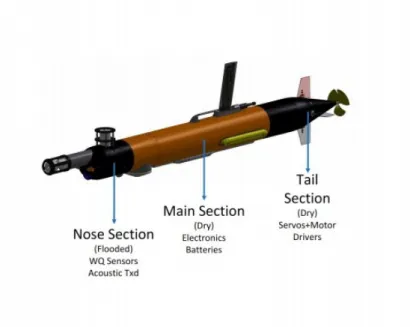
2.3.2 Marine robotic platforms 2.3.2.1 AUV

There are a great number of AUVs in the world. Two examples of them are the ones that have been developed at FEUP.

Figure 2.11: FEUP AUV MARES (Source: htt p : //goo.gl/pxa1B)

One AUV, called Modular Autonomous Robot for Environment Sampling (MARES), was developed by "The Ocean Systems Group"(Oceansys) of FEUP, together with ISR-Porto (Robotic Systems Institute). See Figure 2.11. [16]

According to OceanSys, MARES (Modular Autonomous Robot for Environment Sampling) is a highly modular autonomous underwater vehicle, designed for shallow water operations. The vehicle can be configured to carry a wide variety of oceanographic sensors and includes a set of navigation sensors to ensure that the predefined trajectories are followed.

The characteristics of MARES are in the table 2.1

Table 2.1: Characteristics of MARES Characteristics of MARES

Length 1.5 m

Diameter 20 cm

Weight in Air 32 kg

Depth Rating 100 m

Horizontal Velocity 0 − 2 m/s, variable Autonomy/Range about10 hrs / 40 km

MARES has a very particular feature - the horizontal motion and the vertical motion are com-pletely independent because it is propelled by two vertical thrusters and two horizontal ones. This rare feature makes it possible for the AUV to stay still in the ocean, underwater.

Some features of MARES include:

• On-board location sensors and movement aid; • Modular construction, with reconfigurable sections; • Spare ports to accommodate payload sensors; • Compact and lightweight - fits the trunk of a car;

2.3 Current Underwater Navigation Systems 15

• Robust, with fully shrouded moving parts;

• Operates in confined areas - can ascend/descend in the vertical;

• Autonomous operation, with simple mission definition;

• Rechargeable Li-Ion batteries.

Another very interesting AUV is the Light Autonomous Underwater Vehicle (LAUV) (Fig. 2.12 developed by the Underwater Systems and Technology Laboratory (LSTS). [17] According to LSTS, the LAUV is an Autonomous Underwater Vehicle targeted at innovative standalone or networked operations for cost-effective oceanographic, hydro-graphic and security and surveil-lance surveys.

This lightweight vehicle can be easily launched, operated and recovered with a minimal op-erational setup. The operation of the LAUV does not require extensive operator’s training. It is an affordable, highly operational and effective surveying tool. Starting at a basic functional sys-tem that includes communications, computational syssys-tem and basic navigation sensors, the LAUV capabilities are built up adding optional payload modules. [18]

Table 2.2: Characteristics of LAUV Characteristics of LAUV

Length Starting at110 cm (depends on con f iguration)

Diameter 15 cm

Weight Starting at18 kg

Endurance U p to8 hours @ 3 knots

WiFi 2.4 GHz and/or 5 GHz

GSM/HSDPA Quad− band 3G module

Maximum Depth 100 meters

INS MGB: 1 degree per hour

CT D U p to6Hz sampling rate

Echo Sounder Frequency: 675 kHz (Mounting pointing f orward) Camera Resolution: 720p in H.264 and near 1080p in JPEG Multibeam Frequency: 260 kHz. Range : 100 meters SideScan Sonar Single or dual f requency

Some features of the LAUV are:

• Security and Surveillance;

• Oceanography;

• Hydrography;

• Inertial Navigation.

2.3.2.2 ASVs or ASCs

FEUP has also developed small size autonomous surface vehicles (Zarco and Gama), with a cata-maran shape, designed to operate in quiet waters (rivers, lakes, dams).As mentioned in OceanSys, in its basic configuration, each vehicle weights around 50 kg, and has an additional payload capac-ity of 20 kg. See figure 2.13. The vehicle is actuated by two electrical thrusters and can operate at speeds up to 3 knots. It carries an on-board computer to run fully autonomous or remotely controlled missions, while storing all internal and payload data. A WiFi link connects the ASV to a shore station, allowing for real-time data transmission and mission supervision.

2.3 Current Underwater Navigation Systems 17

Figure 2.13: ASV Zarco (Source: htt p : //goo.gl/pxa1B)

Table 2.3: Characteristics of the ASVs or ASCs Characteristics of the ASVs or ASCs

Length 1.5 m

Width 1 m

Weight in Air 50 kg

Net Buoyancy 50 kg

Horizontal Velocity 0 − 3 knts, variable

Some features of ASCs or AUVs:

• Modular mechanical structure, using COTS elements; • Separation of major modules without tools;

• Spare ports to accommodate payload sensors; • Very stable platform;

• Can operate autonomously or remotely controlled; • Real-time transmission of data to shore.

2.3.2.3 Buoys

The Buoys that are used for navigation and instrumentation are called Navigation and Instrumen-tation Buoys (NIBs). See figure 2.14

NIBs are moored floating platforms with on-board electronics and energy management system. The basic configuration includes rechargeable Lead-acid batteries, a compact GPS receiver and a

low-power radio modem. NIBs can carry a great variety of sensors and transmit data in real time to a shore station using the radio link.

Figure 2.14: Navigation Instrumentation Buoy (Source: htt p : //goo.gl/pxa1B)

NIBs, based on OceanSys, are used as acoustic navigation beacons for the AUVs. In this scenario, they have electronic boards to receive and decode acoustic signals sent by the vehicle and respond by transmitting other coded pings into the water. Since they are deployed in known positions, the vehicle can determine its position by triangulation. During an AUV mission, the buoys also relay navigation information back to a mission control station, allowing for vehicle tracking and mission supervision. [16]

Table 2.4: Characteristics of the Buoy Characteristics of the Buoy

Overall Diameter 75 cm

Weight in Air 30 kg

Net Buoyancy 20 kg

Antenna Height 1 m

2.3.3 Recent Projects

There are many projects currently being worked on related to AUVs in general and evolving to-wards multi-AUVs systems.

2.3 Current Underwater Navigation Systems 19

2.3.3.1 Noptilus Project

One good example of this is the Noptilus Project (NP). The evolution of multi-AUV systems is still in progress of maturing and it still has some flaws when faced with real-life complex situation-awareness operations. These types of operations often involve complex reasoning and demand the ability to make decisions and, as such rely on human beings.

As we are well aware of, any system that involves human beings is bound to have flaws related to the very condition of mankind.

NOPTILUS is a project to fight this flaws. It represents an effective completely autonomous multi-AUV concept which is 100 percent autonomous, thus not relying on humans.

Referring to their own words, in order for this to happen, some advances are required on some aspects:

• Cooperative and cognitive-based communications and sonars (low level); • Gaussian Process-based estimation ;

• Perceptual sensory-motor;

• Learning motion control (medium level):

• Learning/cognitive-based situation understanding and motion strategies (high level). Of extreme importance is the integration of all these advances and the demonstration of the NOP-TILUS system in a realistic environment at the Port of Leixões, utilizing a team of 6 AUV’s that will be operating continuously on a 24hours/7days-a-week basis.

Evaluation of the performance of the overall NOPTILUS system will be performed with em-phasis on its robustness, dependability, adaptability and flexibility especially when it deals with completely unknown underwater environments and unpredictable situations as well as its ability to provide with close to optimal performance. [19]

Chapter 3

Navigation for single Marine Robotic

Vehicles

This chapter describes the single beacon navigation algorithm for single AUVs based on the work of [2]. The algorithm can be split into two main components: the Trilateration and the KF.

3.1

System overview

The system is composed by some principal blocks which constitute the navigation process. See Figure 3.1. Robotic Vehicle Kalman Filter Trilateration Range Computations

Construction of the Virtual Net of Beacons Optimization Position Velocity Optimization output Desired Velocities Estimated Position Velocity

Figure 3.1: System block diagram

3.2

Kinematic vehicle model

To test the single beacon navigation algorithm in Matlab, first a kinematic model of an AUV (in the horizontal plane), was implemented. To this end, a subsystem was defined and implemented as a Matlab block. The inputs of the vehicle block are the linear and angular velocities. The block implements the following equations:

˙ x= vsin(ψ) + vcx (3.1) ˙ y= vcos(ψ) + vcy (3.2) ˙ ψ = w (3.3)

where (x, y) is the vehicle position and ψ its orientation. For simplicity we omitted the third posi-tion coordinate z in the formulaposi-tion. We assume that the AUVs are equipped with pressure sensors that provide the underwater depth. In the equations 3.1, 3.2 and 3.3, we have included explic-itly the current vc= (vcx, vcy), which is assumed to be constant but unknown from the navigation algorithm.

3.3

Trilateration

Trilateration is the process of determining absolute or relative locations of points by measurement of distances, using the geometry of circles, spheres or triangles.

This section describes the several components of the trilateration system. Firstly, there is the formation of the Virtual Net of Beacons, using ranges and displacements that occur in the system AUV-beacon. With this set, we then compute the position of the virtual beacons, which will later be used in an optimization process that gives an estimation of the position of the vehicle that we are looking for.

3.3.1 Forming the Virtual Net of Beacons

To obtain a virtual net of beacons, firstly we proceed to compute the spatial movement of the vehicle from each position to the following one. To do this we integrate the values of the relative linear velocity of the vehicle. In Matlab this was done by implementing the simple discrete formula pk+1= pk+ δ vk where p is the position of the vehicle, δ is the sampling time (which in our case is δ = 0.1s) and v the linear velocity.[2]

The navigation system used consists in one beacon, as mentioned before. However in the process of determining the various positions of the AUV over time, some virtual beacons (VBs)

3.3 Trilateration 23

Figure 3.2: Network of beacons creation (Source: [2])

are created and used in order to make the determination of its location possible. In what follows, we consider a virtual net of beacons composed by N = 4 beacons.

The process begins in the real beacon (P4) that creates the VBs using the displacement made by the vehicle. This is done over 4 different times in 3 different directions. As it is clear from Figure 3.2.

The vehicle obtains the range to the beacon every T seconds (which in our case is T = 4s). This is done by sending an AS, and knowing its speed and time of travel. During the intervals between the range measurements, the vehicle displacement is also saved by integrating the velocity.

After the 4 distances to the beacon are computed, the VBs are created. Firstly, P3 is placed, by doing the inverse motion that the AUV did from t3to t4. This motion corresponds to v(t4− t3). Once computed this motion, and summing to the beacon (P4) we find the position of the first VB (P3). From this new VB we will follow the same logic applying the motion from t3 to t2 (and computing : v(t3− t2)), creating the VB P2and the same goes for the last interval t2 to t1 which creates the VB P1. [20]

3.3.1.1 Position of the VBs

Formally, by following the process described above, the positions of the VBs are obtained accord-ing to:

pi= pN+

Z T_N

ti

v(τ)dτ (3.4)

Where PN is the location of the actual transponder, and v the AUV linear velocity and tithe time when the measurements are taken.

For the particular case of our implementation (N=4) we have

p₄= d(t4) (3.5)

p3= p4+ intv34 (3.6)

p2= p3+ intv23 (3.7)

p1= p2+ intv12 (3.8)

Having computed this, it is time to find the best estimate for the vehicle’s position ¯p. In order to do this, a method of optimization is used.

The expression to optimize is the one that follows and is based on the main reference article for the SB implementation.

¯ p= arg min p∈R2 N

∑

The optimization of a function is the selection of a best element. It consists in maximizing or minimizing the function considered. See Figure 3.3. In our particular case, we are going to optimize the function in (3.9) by finding its minimum. There are several methods used to do this. However, some are more appropriate for some cases than others.

Two typical optimization procedures are • Gradient Descent Method (GDM); • Newton Method (NM).

3.3.2.1 Gradient Descent Method

The GDM is a first-order OM. It is used in order to find local minimum and maximum values, taking steps proportional to the negative or positive gradient of the function at the current point, accordingly.

3.3 Trilateration 25

Figure 3.3: Optimizing a function (Source: http://goo.gl/I9Vba)

• Computing the gradient of f

5 f (x) = ( ∂ ∂ xk

f(x))n (3.10)

For the particular case of (3.9), which is simplified to a form that makes the primitive com-puting easier, we have:

4

∑

∑

∑

Thus, the gradient ∇ f = [hx, hy] is given by

4

∑

∑

• A vector d is a descent for f at x if the angle between the f gradient and d is larger than π, which means that :

5 f (x)T

d< 0 (3.16)

• Direction of steepest descent:

d= − 5 f (x) (3.17)

Gradient Descent algorithm used (3.4):

Figure 3.4: Gradient Descent algorithm

One thing that is of most importance is the picking of the initial condition for the OM. When implementing this, it became obvious that if a wrong or inappropriate initial condition was set the program would never converge to its optimal solutions rendering the entire algorithm useless. For instance, a local minimum can appear and the solution converges to the wrong result.

3.3.2.2 Newton’s Method

The NM has the advantage (when it converges) to have a quadratic convergence. The main idea is to select the descend direction according to which,

The dk becomes:

dk= −[52f(xk)]−15 f (xk) (3.18) where ∇2f denotes the Hessian.

This algorithm has a better stop criterion than GDM, which just considered the number of iterations. To solve this issue, another criterion is added. Now, if the error is of a set value the program stops, meaning we have found a solution that is close enough to the correct value.

3.4 Kalman Filter 27

λ (x) = q

5 f (x)T_[52_f(x)]−1_{5 f (x) (3.19)}

λ2(x) < ε (3.20)

Where λ is the stop criterion.

The algorithm followed in this method is the one that follows 3.5. The only change made, however, were the formulas mentioned above.

Figure 3.5: Newton’s Method algorithm

After some research, the best method to use in this case is neither one of those. To obtain the best results we must use a mixed version of the two. As the NM is the fastest to converge and works with less iterations, it is considered a better method. However, if the matrix of the second primitive is singular, or close to it, it becomes impossible to use this method as we need to invert this matrix in order to implement the method. So, basically, what we do in this optimization is begin by checking if we can use the NM, and use it if possible (matrix singularity), and if not use the GDM; which works in both cases as it doesn’t use matrix inversions.

In the end, the OM in this case is not that important as the results converge fast enough with each method. What becomes the main factor in locating the AUV is the trajectories involved, as will be explained further on.

3.4

Kalman Filter

3.4.1 About the filter

The Kalman Filter is an algorithm that operates recursively, using a series of measurements that contain noise, in order to produce a close-to-optimal estimation.

It uses dynamic models (for example motion equations).

The KF has several advantages when compared to other types of filters,this advantages were crucial to the picking of this type of filter:

• It works recursively (historic is not needed);

• It compensates systematic errors, adapting to alterations in the model (this is particularly im-portant because this system has a lot of possible noise inputs, and also errors associated with measures, discretizations and such) Strength against disturbances in the sensors’ outputs; • It enables the estimation of the complete state of one system, even if not all the variables

have been measured.

Figure 3.6: Kalman filter block diagram

In Figure 3.6 is represented the functioning of the Kalman Filter, which acts as a parallel system to the one we are using, receiving data with noise and sometimes without complete infor-mation. It then proceeds to estimate the values pretended in the respective system.

The process is represented in the generic space state model as:

xk+1= Axk+ Buk+ Gwk (3.21)

With the measurements and observations, y:

yk= Cxk+ vk (3.22)

Where:

• xk - represents the state of the system, which we want to estimate; • uk - represents the input of the optional control;

3.4 Kalman Filter 29

• yk- represents the measures obtained;

• A - is the dynamic matrix that relates the next state of the system k + 1 with k. • B - is the input matrix that relates the input of the optional control with the state x; • C - is the observation matrix and relates the state with the measures obtained yk; • G - is the matrix that models the way the noise affects the system;

• wk- is a random variable that represents the noise in the process; Kalman Gain Kk= Pk−C T (CP_k−CT+ R)−1= P − k C T CP_k−CT_{+ R} (3.23) • K - Kalman gain; • P - Covariance posteriori; • R - Covariance noise.

3.4.2 Kalman filter implementation in this project

After completing the first part of the algorithm we could observe that the trilateration worked, but only without the current’s velocity. Due to the nature of this project, a navigation system that works under those circumstances is almost useless as AUVs always face some kind of current, which affects their motion.

To solve this problem we are going to use a KF, which will estimate the ocean current and also filter the AUVs position. There are many ways of designing KF, ones more suitable than others as some research was needed to understand more about the implementation of such filters [21].

To do this we will consider the ocean current constant and consider the following equations to model the system:

˙

p= vr+ vc+ ξ (3.24)

˙

vc= 0 + η (3.25)

After having the model system defined in the previous expressions it was needed to implement it to a form more suitable of applying the KF. For this, the Euler approximation was applied resulting on the expressions that follow which are ready to be implemented in Matlab and be part of the filter’s algorithm.

      x y vcx vcy       k+1 =       1 0 ∆t 0 0 1 0 ∆t 0 0 ∆t 0 0 0 0 ∆t             x y vcx vcy       k +       ∆t 0 0 ∆t 0 0 0 0       " vrx vry # +ξk " ¯ x ¯ y # k = " 1 0 0 0 0 1 0 0 # k       x y vcx vcy       k +ηk • (x, y) - vehicle position;

• (vcx, vcy) - ocean current velocity;

• (vrx, vry) - water relative vehicle’s velocity; • ¯p( ¯x, ¯y) - position measurement;

• ˆvc - estimative of vcprovided by KF; • ∆T - time step;

• ξk and ηk are assumed to be discrete stationary, Gaussian, zero mean white noise processes and mutually independent.

Figure 3.7 represents, in a block perspective, the different subsystems involved in this SBN system. Subsystem 1 represents the trilateration process, which already "works" in itself but is not at all reliable, needing to be filtered and completed by Subsystem 2, in which the current’s speed enters and the approximation of the position already computed in the previous block. The disturbances represent noise and other errors associated with the process. The output of Subsystem 2 will provide feedback to the system.

The first (Trilateration) and second (Kalman) block (subsystems) are intimately related as they share the use of some values. For example, q, computed on the first block depends on the output of the second one (this is due to the need of the ocean’s current for the position estimation com-puting) and this block, the Kalman one, uses the results of the trilateration, taking in consideration the values of the current and filtering the noise in order to make possible the conversion of the algorithm.

3.4 Kalman Filter 31

Chapter 4

Cooperative Navigation

This chapter addresses the cooperative navigation for multiple marine robotic vehicles. The main idea is to make use of the fact that each individual member of the group could benefit from navi-gation information obtained from other members. For underwater vehicles cooperative navinavi-gation is considerably more challenging but very attractive. Only few vehicles are needed to maintain an accurate estimate of their positions through sophisticated (and expensive) navigation sensors. The other ones can have less sophisticated navigation. [22].

In this chapter, by extending the concept of single beacon navigation for one AUV, we focus in two types of CN:

• The one between an ASC and one or more AUVs;

• The one between various AUVs.

The first one has obvious advantages when it comes to navigation. As there is a ASC located in the sea level, at the surface, it enables the use of GPS to locate the position of the surface, making easier to locate the area where the related AUVs are exploring. These vehicles use, then, another navigation algorithm to compute their location underwater using ASs, in a trilateration system that uses a net of beacons and obtains the location of the vehicle in relation to the ASC. See Figure 4.1.

Figure 4.1: Cooperative navigation between ASC and AUV (Source: [1])

The second one is used in order to have a permanent communication between AUVs which enables the possibility to explore in formation to cover more area and achieve better goals. Another possibility of this CN technique is to make only one of the vehicles to transmit and receive signals to the beacon system and use this navigation information to control the navigation of the rest of the fleet. See Figure 4.2.

Figure 4.2: Underwater fleet navigation (Source: http://goo.gl/D9CJ4)

4.1

CN between AUV and ASC

This type of CN is very attractive because the idea is to use an ASC, which is floating on the water, so above sea level, and for this reason it becomes possible to know its coordinates through the GPS system. The setup proposed is to make the ASC to play the role of the beacon as in the case of Chapter 3. However, in this setup, we will have a moving beacon, as the ASC will be able

4.2 CN between AUV and AUV 35

to move and stay still. Moreover, the ASC can in principle make desirable selected movements to allow a better performance on the computation of the position of the AUV, which is working in exploration, rescue, reconnaissance or such missions. By this we get the position of the AUV related to the ASC, which we have previously located through GPS.

To extend the SBN to the cooperative setup, some modifications in the algorithm are needed. In particular, the computation of the location of the VBN has to be modified by taking into account the displacement of the beacon. More precisely, in our setup with four (virtual) beacons (N=4) we have

p4= pbeacon(12) (4.1) p3= p4+ intv34− [pbeacon(12) − pbeacon(8)] (4.2) p₂= p3+ intv23− [pbeacon(8) − pbeacon(4)] (4.3) p₁= p2+ intv12− [pbeacon(4) − pbeacon(0)] (4.4) • p(0) - position of the moving beacon at the instant t = 0s;

• p(4) - position of the moving beacon at the instant t = 4s; • p(8) - position of the moving beacon at the instant t = 8s; • p(12) - position of the moving beacon at the instant t = 12s;

4.2

CN between AUV and AUV

For different purposes it becomes an advantage to use an AUV as a beacon reference for other AUVs. This can be used, for instance, to guide multiple vehicles in fleet formation for reconnais-sance or rescue purposes. The other vehicles use one AUV as their beacon and can use it as a reference to take their right positions. In environments where few beacons are placed this could have an obvious role and it can also be used mixed with the cooperation with ASCs depending on the purpose we are aiming to.

As this type of navigation involves two or more AUVs, we cannot use the same algorithm as with the previous form of cooperation between systems. This is due to the fact that we cannot rely on the GPS, positioning system as both AUVs will be underwater.

As the position of both vehicles is unknown, and one of them will be the beacon for the other one, we will have to compute the displacement of the vehicle that will serve as the beacon in a similar process as we did before when we implemented the algorithm for one AUV.

Once again, what needs to be changed is how the virtual net beacon is generated and therefore, the calculations of their positions.

The integral of the speed of the beacon-AUV will be computed in order to get its respective displacement and later add it to each according P.

p4= pbeacon(12) (4.5) p3= p4+ intv34− [pbeacon(12) − pbeacon(8)] (4.6) p2= p3+ intv23− [pbeacon(8) − pbeacon(4)] (4.7) p1= p2+ intv12− [pbeacon(4) − pbeacon(0)] (4.8) In this case, the AUV with the beacon needs to have more sophisticated inertial sensors in order to integrate its velocities without accumulating much error.

Chapter 5

Results and discussion

5.1

Single Navigation

In this part, the results obtained throughout the SBN algorithm implementation will be discussed. Some details that should be mentioned about the simulation process are:

• Every 12 seconds, we update the Kalman filter with a new location.

• The sampling time of the overall algorithm is 0.1 s. This time is defined in the configuration parameters.

• It is implicitly assumed that the velocity measurements are obtained at each sampling time. The range measurements are obtained every 4 s.

• For this simulations, we run the program 800s, which was a time we considered appropriate for the AUV to travel enough as to make it easier to be tracked.

For simulation purposes, the path picked for the AUVs movement is a relatively common one. It contains many of the standard types of movements the AUV can have, turning left and right and heading forward and is also realistic as it is the type of paths these vehicles follow when exploring and other similar types of missions.

It is important to stress that several paths were tested during and after implementing the pro-gram because the ability to track the right position and for the algorithm to converge it could be concluded that there are some paths that are better than others. This will be shown clearly in the next figures.

For example, a path that may have some problems is when when the vehicle moves in a straight line away from the beacon and turns out that in this case the location of the positions of the (virtual) beacons are aligned in that a line parallel to the trajectory. In this case, the algorithm may diverge as there is no way of knowing the real distance between the beacon and the vehicle; we just know it is somewhere along that line.

For this reason, as we will see further on, when the navigation is cooperative, with the aid of a moving AUV or ASC, we get better results as we can avoid the greater flaws of this system and by moving the beacon in some "good" directions.

After realising this, some paths were set for the AUV to follow. As expected some with better results than others, but none yet having the best desired results, which are only achieved in cooperation.

5.1.1 Straight Line Movement

Obtained by simply putting the angular speed to zero and keeping the linear speed at 1 m/s.

5.1.1.1 Without noise and without current

To start the simulation of the results of the program implemented in Matlab it was wise to start with the simplest of the cases. In this simulation we can observe the movement made by the vehicle which is coloured in green and we can compare it with the estimated movement obtained by superposing the values of the estimated positions(black dots) of the vehicle using the trilateration algorithm and the Kalman response, given in red. See Figure 5.1.

−90 −80 −70 −60 −50 −40 −30 −20 −10 0 10 −100 0 100 200 300 400 500 600 700 800 y [m] x [m] AUV Position Estimated Pos Kalman Response

Figure 5.1: Line movement without noise or current

5.1.1.2 With noise and without current

After the previous simulation we add some noise to make this simulation more realistic since, when tested in the real world these kind of systems always involve noise. This happens in the sensors , under influence of the environment (storms or such), errors in calculations, so adding it up helps considering these factors. See Figure 5.2.

This problem is easily solved by the filter and does not introduce too much harm to the func-tioning of the trilateration.

5.1 Single Navigation 39 −200 −150 −100 −50 0 50 −100 0 100 200 300 400 500 600 700 800 y [m] x [m] AUV Position Estimated Pos Kalman Response

Figure 5.2: Line movement with noise and without current

5.1.1.3 With current and without noise

Firstly the testing was done without considering the current speed. Later it had to be implemented as it is a crucial factor in this field.

The currents affect greatly the vehicle trajectory and if we don’t consider them in the algorithm, it will not work as it diverges and does not bring any good results.

To be able to compute the position of the vehicle with current speed it is imperative that we use the KF. Due to its capability to act recursively, the KF is used to estimate the current disturbance and use this estimate in order to find the correct location of the vehicle. See Figure 5.3.

−50 0 50 100 150 200 −200 0 200 400 600 800 1000 y [m] x [m] AUV Position Estimated Pos Kalman Response

5.1.1.4 With current and noise

Once again, after the program is tested with current speed we must include noise for realism purposes. See Figure 5.4.

−50 0 50 100 150 200 −200 0 200 400 600 800 1000 y [m] x [m] AUV Position Estimated Pos Kalman Response

Figure 5.4: Line movement with current and noise

5.1.2 Circular Movement

For this movement we keep the same linear speed and give the angular speed a value, in this case 0.1 rad/s.

5.1.2.1 Without noise and without current

The circular motion is better than the linear one because it moves in more directions and is less likely to stay in a "blind angle zone". See Figure 5.5.

−50 0 50 100 150 200 −200 −150 −100 −50 0 50 100 y [m] x [m] AUV Position Estimated Pos Kalman Response

5.1 Single Navigation 41

It presents a good behaviour when it’s not in the presence of current or noise.

5.1.2.2 With noise and without current

With noise, it still has the appropriate response, converging well, just with some minor deviations as it is supposed to have. See Figure 5.6.

−50 0 50 100 150 200 −200 −150 −100 −50 0 50 100 y [m] x [m] AUV Position Estimated Pos Kalman Response

Figure 5.6: Circular movement with noise and without current

5.1.2.3 With current and without noise

When in the presence of current, the movement of the AUV changes, and is no more a perfect circle motion. It still manages to track the position, with a little deviation in the curve which is tight for the few dots we plot. See Figure 5.7.

−50 0 50 100 150 200 250 300 −100 −50 0 50 100 150 200 250 y [m] x [m] AUV Position Estimated Pos Kalman Response

5.1.2.4 With current and noise

With noise, we obtain similar results. See Figure 5.8.

−50 0 50 100 150 200 250 300 −100 −50 0 50 100 150 200 250 y [m] x [m] AUV Position Estimated Pos Kalman Response

Figure 5.8: Circular movement with current and noise

5.1.3 S Movement

This movement is more involved. As we wanted it to go straight for a distance and then curve for a while before going straight again and curve the other way and repeat the motion; we had to implement some code that would create the desired output signal. This code can be found in the appendix.

5.1.3.1 Without noise and without current

In this case the output of the KF tries to follow the movement of the AUV but without much success. It meets paths that are on the blind angle and gets lost in the curves. Clearly calls for a better way to track it, this is solved with a cooperating vehicle, a beacon that has movement. See Figure 5.9.

5.1 Single Navigation 43 −40 −20 0 20 40 60 80 100 −80 −60 −40 −20 0 20 40 60 80 y [m] x [m] AUV Position Estimated Pos Kalman Response

Figure 5.9: S movement without current or noise

5.1.3.2 With noise and without current

Even worse results, as expected. See Figure 5.10.

−40 −20 0 20 40 60 80 100 −80 −60 −40 −20 0 20 40 60 80 y [m] x [m] AUV Position Estimated Pos Kalman Response

Figure 5.10: S movement with noise and without current

5.1.3.3 With current and without noise

It is peculiar how the current speed helps in the convergence of the algorithm. In fact, by giving it another motion, it drives it away from the movements that are harder to track. See Figure 5.11.

−50 0 50 100 150 200 250 300 −50 0 50 100 150 200 250 y [m] x [m] AUV Position Estimated Pos Kalman Response

Figure 5.11: S movement with current and without noise

5.1.3.4 With current and noise

Similar results, but in this simulation the noise helped in some parts of the movement and worsened the others. See Figure 5.12.

−50 0 50 100 150 200 250 300 350 −50 0 50 100 150 200 250 y [m] x [m] AUV Position Estimated Pos Kalman Response

Figure 5.12: S movement with current and noise

5.2

Cooperative Navigation - Between ASC and AUV

For the reasons stated before, the functioning of this algorithm and its implementation in reality is vastly improved with the aid of a moving device, that avoids its weak points. This device in this case will be an ASC, moving in the surface of the ocean, in a movement that is tested by the following simulations as to see what would be a good choice for a ever converging position estimations of the AUV. The movement of the AUV stays the same in every simulation because the S movement is the one used in most operations(reconnaissance, exploration, etc). The reason

5.2 Cooperative Navigation - Between ASC and AUV 45

we tested so many movements in the SN was to better understand what the results would be and in which cases it would have better and worse results.

5.2.1 Straight Line Movement of the ASC

In a research process we tried different movements for the ASC, to find out what would be the best one to use when implementing the program in real vehicles.

5.2.1.1 Without noise and without current

As expected, in a straight line there are many spots that are hard to track, so it gives a poor result. See Figure 5.13. −40 −20 0 20 40 60 80 100 120 140 −100 −80 −60 −40 −20 0 20 40 60 80 100 y [m] x [m] AUV Position ASC Position Estimated Pos Kalman Response

Figure 5.13: Line movement without current or noise

5.2.1.2 With noise and without current

−40 −20 0 20 40 60 80 100 120 140 −100 −80 −60 −40 −20 0 20 40 60 80 100 y [m] x [m] AUV Position ASC Position Estimated Pos Kalman Response

Figure 5.14: Line movement with noise and without current

5.2.1.3 With current and without noise

Once again, the current actually improves the result. See Figure 5.15.

−100 0 100 200 300 400 500 600 −100 −50 0 50 100 150 200 250 300 350 400 y [m] x [m] AUV Position ASC Position Estimated Pos Kalman Response

Figure 5.15: Line movement with current and without noise

5.2.1.4 With current and noise

5.2 Cooperative Navigation - Between ASC and AUV 47 −100 0 100 200 300 400 500 600 −100 −50 0 50 100 150 200 250 300 350 400 y [m] x [m] AUV Position ASC Position Estimated Pos Kalman Response

Figure 5.16: Line movement with current and noise

5.2.2 Circular Movement of the ASC

With a circular movement we get better results than with the straight line, but these are still not the results we are after.

5.2.2.1 Without noise and without current

Still with large deviations, hard to converge. See Figure 5.17.

−40 −20 0 20 40 60 80 100 120 −80 −60 −40 −20 0 20 40 60 80 y [m] x [m] AUV Position ASC Position Estimated Pos Kalman Response

Figure 5.17: Circular movement without current or noise

5.2.2.2 With noise and without current

−40 −20 0 20 40 60 80 100 120 −80 −60 −40 −20 0 20 40 60 80 y [m] x [m] AUV Position ASC Position Estimated Pos Kalman Response

Figure 5.18: Circular movement with noise and without current

5.2.2.3 With current and without noise

Current helps the algorithm convergence, giving better results. See Figure 5.19.

−50 0 50 100 150 200 250 300 −50 0 50 100 150 200 250 y [m] x [m] AUV Position ASC Position Estimated Pos Kalman Response

Figure 5.19: Circular movement with current and without noise

5.2.2.4 With current and noise

5.2 Cooperative Navigation - Between ASC and AUV 49 −50 0 50 100 150 200 250 300 −50 0 50 100 150 200 250 y [m] x [m] AUV Position ASC Position Estimated Pos Kalman Response

Figure 5.20: Circular movement with current and noise

Just to show the results with a bigger circular movement. See Figure 5.21.

−50 0 50 100 150 200 −150 −100 −50 0 50 100 y [m] x [m] AUV Position ASC Position Estimated Pos Kalman Response

5.2.3 S Movement of the ASC

In this case, the ASC follows the AUV right above it, on the surface. This is the movement we were looking for.

5.2.3.1 Without noise and without current Perfect results. See Figure 5.22.

−40 −20 0 20 40 60 80 −80 −60 −40 −20 0 20 40 60 80 y [m] x [m] AUV Position ASC Position Estimated Pos Kalman Response

Figure 5.22: S movement without current or noise

5.2.3.2 With noise and without current Noise is hardly noticeable. See Figure 5.23.

−40 −20 0 20 40 60 80 −80 −60 −40 −20 0 20 40 60 80 y [m] x [m] AUV Position ASC Position Estimated Pos Kalman Response

5.2 Cooperative Navigation - Between ASC and AUV 51

5.2.3.3 With current and without noise

Tracks well the AUV under the influence of the current. See Figure 5.24.

−50 0 50 100 150 200 250 300 −50 0 50 100 150 200 250 y [m] x [m] AUV Position ASC Position Estimated Pos Kalman Response

Figure 5.24: S movement with current and without noise

The next extra figure shows what happens when the vehicle wants to turn back against the current, and has the same speed. As expected the vehicle can’t move against it. See Figure 5.25.

−40 −20 0 20 40 60 80 −100 0 100 200 300 400 500 600 700 800 y [m] x [m] AUV Position ASC Position Estimated Pos Kalman Response

Figure 5.25: S movement with current and without noise

5.2.3.4 With current and noise