Dutch Disease: A Numerical Approach
Marco Miguel June 2013
Dissertation submitted in partial fulfillment of requirements for the degree of MSc in Economics, at the Universidade Católica Portuguesa, June 17th 2013.
ii
Acknowledgements
I am very grateful for my supervisor Professor Maria Isabel Correia that helped me to choose the subject of this dissertation, for all the guidance and comments, for believing in this dissertation and in me since the beginning.
I also would like to thank Professor Teresa Lloyd-Braga and Professor Catarina Reis for their helpful advice and availability.
Last but not least, I would like to thank my family and friends that supported me unconditionally through this experience, especially the ones from Colégio Pio XII. I am especially grateful for my parents, Carlos Miguel and Júlia Afonso that have always tried to do their best in order to provide me the highest level of education.
iii
Abstract
The aim of this dissertation is to develop a model that would allow to analyze under which conditions shocks to the economy can lead to reallocation of labor between sectors and the so-called Dutch Disease, that in this paper is defined as the reallocation of labor across sectors given changes to exogenous variables. It is proved that there are changes in the exogenous variables that do not lead to labor reallocation, and changes in variables such as total productivity factor of tradable goods, relative prices of energy, and net foreign assets, lead to labor reallocation, which under certain assumptions may harm growth. Furthermore, an analysis of Angola’s economy over the last decade is carried out, in where there’s the conclusion that the combined shock in the prices and production of oil have been followed by an expansion of other sectors of production and not a decrease as expected. Therefore, it is possible to show that the cause of the resource curse may not be the Dutch Disease. The assumptions used in the model are presented in the following sections.
iv
Index
1. Introduction ... 1
2. Literature Review ... 3
2.1 Natural Resources Curse: Main Causes ... 3
2.1.1 Rent Seeking ... 4
2.1.2 Volatility ... 5
2.1.3 Dutch Disease ... 7
3. The Case of Angola ... 9
4. The Model ... 13
4.1 Households ... 14
4.2 Firms ... 16
4.3 Government ... 17
4.4 Market clearing ... 17
5. The Solution Method ... 19
5.1 Steady State conditions ... 20
5.2 Permanent Shocks ... 22
6. Numerical results ... 25
6.1 Calibrating the model ... 26
6.2 Main Results ... 29
6.2.1 Improvement in TFP Energy Sector ... 29
6.2.2 Increase in energy prices ... 30
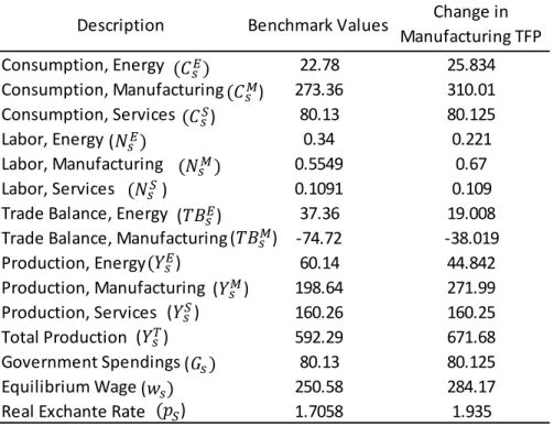
6.2.3 Improvement in TFP of Manufacturing Sector ... 32
6.2.4 Increase in the net foreign assets ... 33
6.3 Different output elasticity of labor in tradable sector ... 34
7. The model versus the Literature ... 34
8. Conclusions ... 37
9. References ... 39
10. NetGraphy ... 42
11. Annex ... 43
11.1 Appendix I-Household Problem ... 43
11.2 Appendix II-Planner Problem ... 45
11.3 Appendix III-Tables ... 51
1
1. Introduction
Countries with higher share of natural resource to GDP may tend to grow less than resource poorer countries. In their influential paper, Sachs and Warner (1995; 2001) show empirically that the abundance of natural resource decreases growth. These results are consistent even when including variables that are considered important to economical growth, as initial income, the trade policy, and investments rates (Sachs and Warner,1995) either geographical or climatic variables (Sachs and Warner,2001).
Despite the lack of a unique reason for this phenomenon, the “Dutch Disease”, has been presented as one of the reasons for bad performance in many resource-rich countries. The “Dutch disease” in that sense is defined as the decrease in the tradable sector (usually manufacturing) due to an increase in the exports of the natural resource sector. This structural change would be optimal in the light of neo-classical theory, as long as that wouldn’t have associated costs (Krugman, 1987). Since the manufacturing sector, or non-resource tradable sector is seen as the one that creates the externalities to production, the decrease in this sector is considered suboptimal and leads the economy to incur costs related to the loss of competitiveness and in that way to lower growth and even negative growth (Krugman, 1987; Sachs and Warner, 1995). This fact is a concern if the shock is temporary wish leads to a shrinking of the non-resource tradable sector, and loss of its comparative advantages. When the resources run out, it would be difficult for the sector to regain its comparative advantages (Krugman, 1987).
Corden and Neary (1982) presented a model with three sectors, two tradable and a non-tradable in which one of the tradable sectors is the extractive kind and the one that faces an improvement in technology. In their simplest model, with labor being mobile between sectors and capital sector-specific, Corden and Neary (1982) found that after a boom in the resource sector that leads to a decrease in output of manufacturing and a deterioration of trade balance in this sector, and leaves place to real appreciation (the exchange rate is defined as the relative price of services in terms of manufacturing).
The aim of this dissertation is to analyze the effects related to unexpected changes of growth that can lead to structural change, and eventually to the Dutch Disease. In the
2
presented model, given the assumptions that the shock is permanent, there is full employment, and there are no costs associated to labor movement across sectors, the shocks will always lead to equilibrium with higher total production, and because of it, the
Disease in this paper is simply defined by the movement of labor across sectors. To
achieve that, the model developed in this dissertation tries to replicate the results found by Corden and Neary (1982). The model is able to replicate most of the results presented by the authors such as the de-industrialization effect, given by lower output in the manufacturing, and the real exchange rate appreciation.
Lastly, the case of Angola, which is a resource-rich country that has been performing badly since the 70’s is discussed. However, since the end of the war in 2002, the country has been performing quite well, given the combined effect of prices and production of Oil, which have been growing since 2000. Besides that and despite the growing of the natural resource sector, the country has also been registering robust growth in the other sectors, specifically; manufacturing, agriculture and also as expected in services.
The plan of this paper will be: Section II the literature review in which the main facts about resource curse and possible causes are presented, Section III presents the case of Angola, in Section IV the model is presented, Section V is the calibration of the model, in Section VI the main results of the model’s simulation are presented, Section VII is presented a comparison between the model and the literature, Section VIII conclusion.
3
2. Literature Review
2.1 Natural Resources Curse: Main Causes
It is expected that countries with large endowment of resources would have higher growth rates than countries that are resource-poor, since the resource availability increases national wealth which may result in investments and growth (Sachs and Warner, 1995). However, empirical evidence shows that most of resource-rich countries have experienced lower growth than resource-poor countries and in some cases have experienced negative growth rates (Davis, 1995; Sachs and Warner, 1995; Rodriguez and Sachs, 1999; Van der Ploeg, 2011). According to Van der Ploeg (2011, p.471) from the 65 resources-rich countries analyzed, only four (Botswana, Thailand, Indonesia, Malaysia) where able to achieve growth rates above 4 percent.
The most evident cases of resource-poor countries that performed better are the Asian, such as South Korea, Japan and Taiwan which have been outperforming resource-rich countries like Mexico, Nigeria, and Venezuela.
Sachs and Warner (1995) established an inverse association between resource intensity and growth, but were not able to establish the main causes of it, even after controlling for several variables such as initial income per capita, investments, bureaucratic inefficiency, among others. They founded that resource-rich countries grew on an average about one percent less than their counterparts between 1970 and 1989.
Collier and Venables (2008) found that in the short run, shocks to commodity (non-agricultural) prices lead to an increase in short run growth rate, but in long run the effects are negative. Additionally, they found that the negative effect is conditional to governance, that in cases of countries with good governance as is the Norway, Australia and Botswana’s case, the results of shocks in prices are positive even in the long run, but for countries that have bad governance the impact on price is generally negative.
Similar results are also discovered by Sala-i-Martin and Subramanian (2003) where the management of Oil revenues is analyzed in Nigeria. They concluded that in this case the main reason for the bad performance was the rent seeking behavior, which can be
4
translated into corruption, the appropriation of national wealth by the successive dictatorship in the country which transferred huge amounts of wealth to tax havens. Therefore they conclude that apart from the appreciation of the exchange rate, the real problem of bad performance is related to the malfunction of legal institutions in the country (Sala-i-Martin and Subramanian, 2003), a conclusion that is also shared by Mehlum et al. (2006).
Given the above literature, it may be concluded that the prime causes of the natural resource curse phenomenon are rent seeking behavior, volatility of resources prices, and the "Dutch Disease" (Sachs and Warner 1999; Van der Ploeg ,2011; Oomes and Kalcheva, 2007). In the next section each of these points are briefly analyzed, and special attention is given to the Dutch Disease which is the focus of this paper.
2.1.1 Rent Seeking
According to Murphy et al (1993, p.409) Rent Seeking is "any redistributive activity that takes up resources". Rent seeking can be either private or public, where private is related to litigation, theft or other forms of transfers between private agents, while public rent-seeking is related to transfers from the private sector to the government bureaucrats, or from government to the private sector (Murphy et al., 1993).
Rent-seeking activity presents an increasing return to scale, and as result, the weaker the legal institutions and property rights are, the higher will be the number of agents that will engage in this activity instead of productive activities (Murphy et al., 1993; Lane and Tornell, 1996).
As stated by Philip and Tornell (1996, p.214) when rent seeking is intense it decreases the return of the investment, mostly due to the fact that investments are not chosen in the perspective of efficiency, and as result the overall growth rate of economy decreases (Murphy et al., 1993). They named this effect as voracity effect, which "is a more than proportional increase in redistribution of response to a windfall".
The main channel that rent seeking activity constrains growth is through innovation (Murphy et al., 1993). In a context of weak institutions and lack of property
5
rights, companies may find more barriers (licenses, permits, among other public goods) to entry, given the corruption, which increases the total set up cost, deterring new entries and more competition which result in less diversification and innovation (Murphy et al., 1993; Shleifer and Vishny, 1993; Tornell and Lane, 1998).
Bribery acts as a fee that is a distortionary tax which is paid by the new or existing companies, channeled to individuals and not to the government (Shleifer and Vishny, 1993; Murphy et al., 1993). As a result, the domestic and foreign direct investments are lower (Shleifer and Vishny, 1993).
While in Sachs and Warner (1995) the effect of institutions was not important to explain the resource curse, Mehlum et al (2006) found that the difference between growth performances across resource rich countries is dependent on the quality of the institutions. As presented by Mehlum et al (2006, pag.16), a combination of grabber friendly institutions and resource abundance leads to lower economic growth, while producer friendly institutions allow countries to benefit from their resource through high growth rates. This fact can be easily seen in countries as Botswana, Norway, Australia that are resource rich and had benefited from it, while countries like Angola, Nigeria, Zambia, among others have failed to transform the abundance of resource in overall in sustained growth Mehlum (2006). The first group of countries are well known for the quality of institutions, being among the less corrupt countries according to the corruption perception index (Transparency International, 2012), while the second group is mostly in the bottom of the same index.
2.1.2 Volatility
Cavalcanti et al., (2012) found out in their study that the dependence upon resources is not the cause of lower growth, since it does not affect directly the TFP (Total Factor Produtivity). He found that the channels in which volatility lowers the growth are in fact that commodity prices may harm the capital accumulation (either physical or human).
Using two data sets, one with 92 countries and other with 24 OECD countries Ramey and Ramey (1995) discovered that there is a negative relationship between
6
volatility and growth, in which one standard deviation of volatility would imply a decrease in growth of about one half in the 92 countries data set, and one third of OECD countries.
It is also stated that resource dependence can be a curse or not depending on the economy composition. On a diversified economy, with a strong financial sector (as Norway) it is a benefit, while in less diversified countries, as Nigeria which are highly dependent on primary goods exports are more prone to “ boom and bust” periods (Van der Ploeg and Poelhekke, 2009).
Hausmann and Rigobon (2002) shows that if the non-resource tradable sector is large enough, the relative prices can be stable even when considering cases where there is much volatility generated by the resource tradable sector. Otherwise, if the non-resource sector is small the shocks related to the resource income will not be accommodated through movement in the labor market, but by expenditure-switching (Hausmann and Rigobon, 2002).
Van der Ploeg and Poelhekke (2009, p.14) found that "countries that are closed to international trade, have a bad financial market, are landlocked and have a high share of natural resource exports have higher volatility in unanticipated growth in output per capita and therefore worse growth prospects".
Most of Africa’s resource rich countries share the characteristics mentioned by Van der Ploeg and Poelhekke (2009, p.14), Combes and Guillaumont (2002), and as result in their study they found out that the resource rich African countries had lost per annum about 2.98% in growth (in the period 1970-2003) when compared to the South-East Asian due to high volatility of unanticipated growth. In that sense volatility may be the main cause for bad performance, and not the abundance of the resource itself (Van der Ploeg and Poelhekke, 2009; Cavalcanti et al. 2012).
However if a country that is facing a windfall of resources decides to save them, for instance in a fund, either stabilization or saving funds (also known as Sovereign Wealth Funds), in order to minimize consumption, the effects related to the resource curse may not exist (Sachs, 1995).
7
2.1.3 Dutch Disease
The Dutch Disease is generally presented as one of the main causes for lower growth rate in some resource-rich dependent countries and will also be the main focus of this work. As presented by Corden (1984, p.359) "The term Dutch Disease refers to the
adverse effects on Dutch manufacturing of the natural gas discoveries of the nineteen sixties, essentially through the subsequent appreciation of the Dutch real exchange rate".
It is caused when there is a boom in one of the tradable sectors of production, leading to a movement of resources (physical and human) from the non-boom sector to the booming sector, causing an increase of production on the former, while the latter decreases. This boom main be caused by shocks in productivity, in the international prices of tradables, external Aid or foreign direct investment (Corden and Neary, 1982; Corden, 1984; Torvik, 2001).
In their influential work Corden and Neary (1982) present a model with three sectors, two sector producing tradable goods (as manufacturing and energy, respectively) and one sector that produces a non-tradable good (as service).
They showed that a permanent Hicks Neutral shock in the technology of the energy sector, has two effects, the first one is the movement effect (Corden and Neary, 1982; Van Wijnbergen, 1984) which implies a transfer of resources (human and physical), from the non-boom sectors of the economy to the boom sector (Corden, 1984; Corden and Neary, 1982; Davis, 1995), and there would also be a real exchange appreciation (an increase in the prices of services relative to prices of manufacturing). The resource movement in that way affects the services and manufacturing, leading to a lower output in both sectors.
The boom promotes an increase in the aggregate demands of goods due to the higher real marginal returns on capital in the boom sector, simultaneously increasing the demand for all goods. The increase in demand for the manufacturing goods will be satisfied by increasing in imports, leading to a deterioration of the trade balance.
As a result of the movement effect, the output in the manufacturing sector and services sector will decrease and so that leads to the phenomenon known as direct
8
de-industrialization (Corden and Neary, 1982; Corden, 1984; Oomes and Kalcheva, 2007; Van Wijnbergen, 1984; Sachs and Warner, 1999).
The higher demand for services leads to an exchange rate appreciation that draws out further resources from manufacturing (and under some assumptions can even draw out resources from the boom sector) to the services, a fact that deepens the loss of
competitiveness in the manufacturing sector, allowing the rise of the
indirect-industrialization (Corden, 1984; Corden and Neary, 1982).
While the effects of the boom to the manufacturing sector are undoubtedly a decrease in the output, the same (cannot be applied to the services sector, since the movement effect may lead to a decrease in output, but the spending effect will lead to an increase in output (Corden and Neary, 1982). The importance of the dominant effects is dependent on the consumption of services in the economy.
However, the de-industrialization process may not completely offset the growth effects from the increasing output of the boom sector. As aforementioned, the service sector may experience a higher output and this effect combined with the increase in energy can offset the negative effects on the loss of productivity in the manufacturing sectors (Davis, 1995).
The following de-industrialization can be seen as the result of efficient resource reallocation and market adjustments due to higher marginal productivity of capital, and in that sense should not be seen as unpleasant to the economy (Davis, 1995), and in some cases it may even lead to a higher overall output.
However, generally, most of the economic growth is attributed to Learning by Doing, which may be translated as investment in human capital that is specific of a sector but not appropriate by individual firms (Gylfason et al., 1999; Van Wijnbergen, 1984; Krugman, 1987; Torvik, 2001). The Learning by Doing is assumed to be specific of the tradable sector (mainly the manufacturing) in the papers presented by Gylfason et al. (1999), Van Wijnbergen (1984) and Krugman (1987) and that is the case if the resource windfalls are not permanent, but are long enough to promote an adjustment in the market that will be difficult to reverse after the windfall is exhausted, the economy would
9
be worse (Krugman, 1987; Van Wijnbergen, 1984; Rodriguez and Sachs, 1999).
Therefore, increasing the productivity of primary sectors (excluding agricultural) increases the real exchange rate, and as a result, decreases the profitability and investment in manufacturing, reducing the human capital accumulation, and in that way damages growth (Gylfason et al., 1999). Using a data set with 125 countries, from 1960-1992, Gylfason et al. (1999) found out that an increase in part of primary exports in labor force from 5% to 30%, may lead to a decrease of growth per capita of about 0.5% per annum.
In order to avoid the loss of competitiveness in the manufacturing sector, the government may subsidize the companies, with part of the revenues from the windfall that have the potential to generate learning by doing effects (Van Wijnbergen, 1984).
On the other hand, Torvik (2001) defends that both sectors are able to induce learning by doing and there is also the spillover of it from one sector to another, in this case the increase in productivity would lead not to a de-industrialization but to a pro-industrialization.
This study uses a static general equilibrium model to analyze the impacts of changes in variable as prices and productivity to analyze the change produced in equilibrium. Since the analytical solution is very complex and makes it difficult to analyze the impact on some variables, as the system uses multiple variables, the numerical approach was implemented to draw some of the conclusions.
The main use of this model is, as stated before, the understanding of resources reallocation due to shocks in the economy.
3. The Case of Angola
Angola is a Sub-Saharan African country, with an estimated population of about 20 million (World Bank, 2013) which gained its independence from Portugal in 1975, but after that sank in a civil war that lasted about 30 years, ended in 2002. Since 2002, favored by the end of war and by the higher production of oil and its high prices, where the oil prices for the OPEC (Organization of the Petroleum Exporting Countries) basket, which Angola is
10
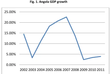
member, achieved a maximum of USD 140, being the main exportation product, led the country to a robust growth from 2004 to 2008 (Fig.1).
Fig. 1. Angola GDP growth
Source: World Bank Database
This growth was also boosted by a growing non-oil sector, experiencing growth rates close to the oil-sector from 2002 to 2008, of about 7% (Centro de Estudos e Investigação Científica, 2008). Despite the dependence on Oil decreasing over the time, it’s still highly dependent, where the production in the GDP was more than 50 percent until 2009 (Banco Nacional de Angola, 2013). Besides the lower value, less than 50% since 2010, it is still above 40%, and the exposure of the country to international shocks is high, as it can be seen by the financial crisis. Due to financial crises and technical issues, the Oil production dropped by 5% in 2009, 2% in 2010 and 5% again in 2011 (Banco Nacional de Angola, 2013). The growth rate during the same period was, 2.39%, 3.39% and 3.40% (Banco Nacional de Angola, 2013; World Bank, 2012) respectively.
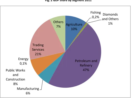
The positive growth rate was due to non-oil sector, mainly construction, agriculture and energy on which each grew on an average of 15% in the same period (Banco Nacional de Angola, 2013). The main source of public revenues is still from oil revenues, which represents more than 40 percent of GDP in 2011 (Fig.2), while the revenues from tax on the sectors still are less than 15%.
0.00% 5.00% 10.00% 15.00% 20.00% 25.00% 2002 2003 2004 2005 2006 2007 2008 2009 2010 2011
11
Fig. 2 GDP share by segment 2011
Source: CEIC, Relatório Económico de Angola
The country is the second major oil producer in the African continent, only after Nigeria, with a production of about 1.9 million of barrels (African Economic Outlook, 2012). Being the main economic driver and capital-intensive, it may constrain economic development since it has a small role in job creation, it employs less than 1% of total labor force as seen in Fig.3 (African Economic Outlook, 2012; Centro de Estudos e Investigação Científica, 2011). This fact is easily seen in the growth rate of employment which has been increasing way below the economy. The highest growth rate in labor force was about 7% in 2006, while at the same year the growth rate of output was about 21%. The period 2006-2011 Angola registered an average growth rate of output at about 11% while the growth rate of labor force was only about 4%.
Agriculture 10%
Fishing
0,2% and Others Diamonds 1% Petroleum and Refinery 47% Manufacturing 6% Public Works and Construction 8% Energy 0,1% Trading Services 21% Others 7%
12
Fig. 3.Labor Force Distribuition (Average 2005-2011)
Source: CEIC, Relatório Económico de Angola
It is important to note that despite the increasing production and prices of oil, the other sectors have been increasing substantially, mostly in agriculture, construction and energy (non-oil). These results show that increases in one of the tradable sector, even in the non-labor intensive sector may not lead to the Dutch Disease at least in the short run. As stated by Corden and Neary (1982), the predominant effect in countries that are oil producers is the spending effect, creating a demand of all goods in the economy. In this case this income effect allowed the increase of production in the manufacturing and services, mainly caused by public demand and also by the oil sector.
The oil sector still is the main driver of the country exports, representing about 90% of all exports (Centro de Estudos e Investigação Científica, 2007). The diamonds are the second source of exports with an average of 5%, and goods as refined products, gas, laminates fishery and coffee which represents only about 5% of the total exports. Although the main source of employment is agriculture which is for internal consumption, its low productivity in the sector still is predominantly familiar (CEIC, 2007). The mechanized agriculture covering only about 2%, of the total cultivated area (Centro de Estudos e Investigação Científica, 2011), meaning that more than 97% of the agriculture
84.43% 0.23% 0.58% 0.65% 0.09% 3.57% 5.13% 5.30%
Agriculture, forestry and fishing
Petroleum and Refinery Diamonds and others Manufacturing sector Energy and water Public works and construction
13
still is carried forward using rudimentary techniques. Another factor that harms significantly the sector is the migration of young workers to cities, leaving the production to the old and female workforce (Centro de Estudos e Investigação Científica, 2011). And the lower level of fertility must be taken in account (Centro de Estudos e Investigação Científica, 2011).
In the next section the main assumptions of the model is presented.
4. The Model
The model represents a small open economy with three sectors, where the net
international interest, given by rt (which is assumed to be the same across sectors), is
exogenous to the economy. The economy is said to be small because it is not able to influence the world prices on neither the tradable goods nor the real interest rate. Markets are competitive. There is the production of three goods, where two are tradable
and one is non-tradable1.
The tradable goods are energy ( E
Y ) and a manufacturing ( M
Y ), while the
non-tradable good is services ( S
Y ). Despite the fact that some categories of services can
be tradable, and some manufacturing can be non-tradable, in the model services it is assumed to represent every non-tradable good and manufacturing to represent the tradable goods besides energy. Every technology i is described by a neoclassical
production function that uses as inputs labor, i
N and capital, i
K .
Labor is mobile across sectors, and there is no international labor mobility, but we can exclude the possibility of migrations. Capital is sector-specific, the initial stock of
capital,K0, is given and there is no capital accumulation, which restricts the analysis to
stationary environments. This assumption allows us to focus on the re-allocation of labor across sectors, which we assume is behind the notion of Dutch Disease, buying us simultaneously a very tractable model. Labor is supplied inelastically and money plays no
role in the economy. Total factor productivity is exogenous and is represented by i
A in
14
every sector .i It is assumed to be multiplicative in the production function, as Hicks neutral productivity. The households own the firms and can save through external assets
represented by ,B that has a real return equal to international interest rate, rt. The
government spends a fixed amount of Gt non-tradable goods, and uses a lump sum tax
t
to finance its spending.
This model allows to study the changes in general equilibrium through permanent shocks in the total factor productivity of every sector, namely energy, what would allow us to study the so-called de-industrialization, and the effects on real output, and in this way confirm or not the "Dutch Disease" theory. The main specifications of the model are given below.
4.1 Households
There is one infinitely lived representative household with preferences over
consumption of sequences M
t
C for manufactured goods, E
t
C for energy good and S
t
C ,
for services goods. The lifetime utility2 is given by the following function:
( ) ( ) ( )
, 0< <1 ln = 1 2 3 0 = S t E t M t t t C C C U
(1)The households supply inelastically N units of time to work in the market. The
budget constraint is given by:
t S t St E t Et M t S t St E t Et M t t t t a r Y p Y p Y C p C p C a1 = (1 ) (2)
Where at1 is the private net foreign assets holdings, t refers to tax paid to the
government by the households and rt is the international interest rate. The factor
prices, taxes and wealth are measured in terms of manufacturing goods, pMt, which is
2 The utility function is differentiable at least twice and has the following properties: 1) U'()>0, U''()<0;
=0,limCiU' Ci lim
=' i i
C U C ; 2) is the discount factor and i >0 is the proportion
15
used as numeraire, and normalized to one. pSt is the relative price of services in terms of
manufacturing, and pEt is the relative price of energy in terms of manufacturing.
In the budget constraint total income is given by the production of every period. Using the
definition of = ti t* i i, it t i t N r K p w
Y wt, the return of labor factor in units of the
manufacturing and rt the return of the stock of capital, in units of the manufacturing,
are exogenous to the household as well as i
K . Since markets are competitive profits are
zero. The total return on labor is also exogenous since labor is in elastically supplied. Then using the value of production in the budget constraint is equivalent to using the factors return of each sector.
The Household problem is then given by:
( ) ( ) ( )
0< <1 ln max 1 2 3 0 = S t E t M t t t C C C
subject to: t S t St E t Et M t S t St E t Et M t t t t a r Y p Y p Y C p C p C a1 = (1 ) (3) andThe No-Ponzi game condition for households is:
1
0 lim 1 = 1
j T j T T r a (4)The static FOC are given by:
Et M t E t p C C 1 = ) ( ) ( 2 1 (5) St M t S t p C C 1 = ) ( ) ( 3 1 (6) The dynamics FOC conditions are given by:
) (1 = 1 1 t M t M t C r C (7) ) (1 = 1 1 1 t Et Et E t E t r p p C C (8)
16
These FOC plus the budget constraint (3), comprise the set of conditions that determine
the households choices when a0=a0 , and the transversality condition holds as:
1
=0 lim 1 = 1
j T j T T r a (9)4.2 Firms
Firms are price takers, in goods markets and the labor market, and operate with one of the three available technologies. These technologies are Cobb-Douglas functions, in which the inputs are labor and capital for all the sectors.
1 < < 0 , ) ( ) ( = 1 M t M M M t A K N Y (10) 1 < < 0 , ) ( ) ( = E E 1 tE E t A K N Y (11) 1 < < 0 , ) ( ) ( = S S 1 tS S t A K N Y (12) where i
A is the total factor productivity (TFP) of sector i , which is exogenous, i
K is
the capital in each sector and i
t
N is the labor in each sector, where i=M,E,S3. In each
period the firms maximizes:
i t i t it t i t i K r N p w Y * = max subject to: b i t b i i i t A K N Y = ( )1 ( ) (13) for i=M,E,S and b=,,
FOC for those firms are given by:
Manufacturing: t M t M w N K A 1( )1 = (14)
3 The production function is neoclassical, meaning that the following properties must hold:
1) CRS: Fi(Ki,Ni)Fi(Ki,Ni) for any K, L and λ>0; 2) Twice differentiable, with
0 ; 0 i K i N F F and 0; NNi 0 i KK F F ; 3) Satisfy (0, ), Ki(, i)0 i i K N F N F 0 ) , ( , ) 0 , ( Ni i i i N K F K F .
17 Services:
St t S t S S p w N K A 1( )1= (15) Energy: Et t E t E E p w N K A ( )1( )1= (16)Notice that, we are assuming that capital is constant across time and firms. Equalizing equations (14)-(16) gives the optimal allocation of labor across sectors as below:
1 1 1 1 1 1 ) ( = ) ( ) ( = ) ( = tS S S St E t E E Et M t M t A K N p A K N p A K N w (17)4.3 Government
The model assumes that Gt is the government spending in non-tradable and that
there are lump sum taxes, then the model has Ricardian equivalence, and without loss of generality it is assumed that government does not borrow or lend. The government budget constraint is balanced every period, which imply that the government budget constraint can be written as:
t t
G = (18)
4.4 Market clearing
• Labor MarketLabor is allocated in manufacturing sector M
t N , energy sector E t N , and in services sector S t
N according to the equilibrium condition given by equation (17). Labor
supply is inelastically constant over time and given by N. The labor market clearing
implies: S t E t M t N N N N = (19) • Goods Market
The output of tradable sectors, as well as imports in those sectors are used for private consumption and can be exported, while the output of non-tradable sector is used
18
for private and public consumption. There is no investment, and the value of capital is
fixed in every period. Assuming that g S
t t
Y G
which is the share of government’s
spending in the production of non-tradable.
M t M t M t C TB Y = (20) E t E t E t C TB Y = (21) g C G C Y S t t S t S t 1 = = (22) Where i
TB is the trade balance and is given by difference between exports and imports
)
(EX IM , for i=M,E.
• Assets
Under the assumptions that there is only private savings, private wealth can be defined as:
K B
at = t (23)
And the accumulation of net asset holding, in units of M, is given by:
M t E t Et t t t B r p TB TB B1= (1 ) (24)
where Bt is the foreign net assets holdings, and
t
r the international interest rate.
• External sector
The current accountCAt, in units of manufacturing, is given by:
M t E t Et t t t B r p TB TB CA = 1 1 (25)
In absence of shocks the economy is in a stationary equilibrium implying a current account equal to zero and therefore:
s s M s E s EsTB TB Br p = (26)
where subscript s stands for steady state.
In the next section the general equilibrium is solved using the central planner problem.
19
5. The Solution Method
The general equilibrium can be solved using the solution of a central planner problem, constrained by the constant value of g . The condition that allows to determine
the equilibrium4 is now presented.
The central planner will choose the optimal value for
= 0 = 1 , , , , , , , , t tt M t E t S t E t M t S t E t M t C C N N N TB TB BC that solves the following problem:
1 2 3
0 = ) ( ) ( ) ( ln S t E t M t t t C C C Max
subject to: M t M t M t M M TB C N K A ( )1( ) = (27) E t E t E t E E TB C N K A ( )1( ) = (28)
g C N K A S t S t S S 1 = ) ( 1 (29) N N N N tS E t M t = (30) ) (1 = 1 E t t t t Et M t p TB B B r TB (31)
0 1 lim 1 = 1 Tj j T T r B (32) givenB0.The solution of this problem is summarized by the following conditions:
1 1 1 1 2 1 ) ( ) ( = ) ( ) ( M t M M E t E E M t E t N K A N K A C C (33)
1 1 1 1 3 1 ) ( ) ( ) (1 = ) ( ) ( M t M M S t S S M t S t N K A N K A g C C (34) Et M t E t p C C 1 = ) ( ) ( 2 1 (35) Equations (33) and (34) show that marginal rate of substitution and marginal rate
20
of transformation must be equal in every sector. And equation (35) imposes that the marginal rate of substitution equalizes the terms of trade that is the marginal rate of transformation through trade. This condition is also part of the planner equilibrium because the relative price of energy is exogenous to the planner, since it is an international exogenous price.
The dynamics equations for the planner are given by: ) (1 = 1 1 t M t M t C r C (36) ) (1 = 1 1 1 t Et Et E t E t r p p C C (37)
The transversality condition is given by:
=0 1 lim 1 = 1 Tj j T T r B (38)In summary conditions (27)-(31) plus conditions (33)-(38), given B0 determine
the central planner allocation.
5.1 Steady State conditions
In this section the stationary equilibrium conditions are described. Assuming that the rest of the world is in the steady state and preferences are identical to our economy,
then (1rt)=1 and =1 1 Et Et p p
(so the relative price of energy is constant over time
and given by pEt = pEt1 = pE) and from equations (36) and (37)
i s i t i t C C C = 1= for E M
i= , . By these assumptions the system can be reduced to:
Combining equation (33) and (35) it is imposed that MRTS is equal to the terms of trade.
0 ) ( ) ( = 1 1 1 1 1 t N K A N K A p M s M M E s E E E (39) Substituting equations (19), (34) into (35) and combining with (29) it reduces to:
= ( ) 0 ) ( ) (1 2 1 1 3 N N N t N K A g p C E s M s M s M M E E s (40)21
Substituting equations (26), (27) and (34) in (30) gives:
( ) ( )
( )
= 1 (1 ) 0 1 2 1 1 t r B B C N K A p p C N K A t t t E s E t E E E E E s M t M M (41)In the stationary equilibrium as Bt1=Bt =B0, the equation becomes:
( ) ( )
1 ( )
= 0 1 2 1 1 t r B C N K A p p C N K A E E E E sE sE s E s M s M M (42) Therefore if the system is reduced to the equations (39), (40) and (42) it allows toobtain values for M
s E s E
s N N
C , , . Using these allocations, it is possible to find the
equilibrium values for the others variables. Using the results found for , , sM,
E s E
s N N
C the
equilibrium value for M
s
C is given by (33); the equilibrium value of S
s
N can be
calculated given the equation (30) and therefore the value of S
s
C from equation (35); the
values for M
s
TB and E
s
TB are given by equations (27) and (28) respectively. The
relative price of services is determined by:
M sM S M S s S S p N K A N K A 1 = ) ( ) ( 1 1 1 1 (43) and real wage by the equation of optimal labor allocation, equation (18).Using the mentioned equations, it is possible to analyze how changes in equilibrium may lead to a reallocation of labor across sectors. The initial stock of capital is
given by Ki =1, for i=M,S, while for the energy sector it will assume different values
from the unit which will be clarified in the calibration section.
From these conditions it is already possible to draw general conclusions, which are stated in the following propositions.
Proposition 1: Assuming that pE is constant and that (1 )=1
rs
the
economy is in steady state if ̂ and g is constant.
Proof. If ̂ ̂ then it is true that (42) is the one restricting the equilibrium.
As we saw the conditions for relative price of energy and the relation between interest
22
it means that equilibrium equation (39), (40) and (42) determines that ̂ therefore the
economy is in a steady state. Changes in i
A , B0 and pE would lead to a new
stationary equilibrium with labor reallocation. The relative price of services is also
constant over time for a given value of i
A, B0 and pE, using equation (43).
Proposition 2: If the TFP of all sectors changes by the same proportion the economy is on a balanced growth path, with a constant labor allocation across sectors, when B0 =Bs =0.
Proof. A common growth rate in overall TFP, would not change the equilibrium values of
, , sM E s N
N when B0 =0, (1r)=1 and ̂ ̂ The MRTS between energy and
manufacturing are constant as well as the MRTS between service and manufacturing, equation (44). In that way no changes would occur in the relative prices of energy or
services, resulting that ̂ and that ̂ Since there are no changes in relative
prices of services, the changes in wages across sectors are equal to change in TFP, given as
̂ ̂ . This can also explain why there is no labor reallocation and ̂ .The
production changes in every sector by ̂ ̂ for i=M,E,S.
5.2 Permanent Shocks
Being the main question to answer by this model labor reallocation is described, first in general terms and after numerically, how can we characterize labor reallocation due to permanent shocks.
Proposition 3: Increasing non-tradable TFP relatively to tradable TFP does not lead to labor reallocation.
Proof. From equilibrium conditions, (39), (40) and (42) it is possible to verify that
changes in services TFP do not enter into these equilibrium conditions. Therefore a
permanent change in services TFP, AS, will not change the allocation of labor in the
manufacturing or energy sector in this way ̂ ̂ and consequently, ̂ . In
the new equilibrium, the relative price of services should decrease in the same proportion
23
̂ [ ̂ ( ) ̂ ] ̂ ( ) ̂ (44)
Also using equation (29) ̂ and implicitly, ̂, will change so the market clearing
condition for services holds. The intuition behind the above results is that increases in the non-tradable sector TFP’s leads to a higher production of those goods, completely compensated by the decrease of the relative prices of non-tradable that we must change in order to restore the equilibrium. As result the production in the tradable sector in unchanged.
The final equilibrium would have a higher output and consumption of services, which is obtained due to lower relative price of services, but without labor reallocation and with no changes in the tradable sectors output. From these results, it can be concluded that the effects related to the Dutch Disease aren´t caused by changes in the technology of non-tradable sector. After describing the effects of changes in TFP of non-tradable, changes in TFP of tradable sector will be assessed.
Proposition 4: Permanent changes in the level of energy prices have identical effects on equilibrium than permanent changes in energy TFP, except for the equilibrium value of energy consumption, both will lead to labor reallocation.
Proof. From equation (39), (40) and (42) it is possible to see that M,
s N E s N and E s EC
p do not depend separately on pE and
E
A but on the product pEAE. Changes
in E
EA
p lead therefore to identical effects in the labor re-allocation across the tradable
sector, and between these and the non-tradable sector. Changes in E
EA
p also have an
effect on pECsE. Whether the equilibrium is changed due to a new pE or to a new
E
A
is just on CsE. Within the tradable sector, the increase in relative prices of energy lead to
a lower consumption of energy, while it has a positive impact in the consumption of manufacturing, when compared with an increase of the energy TFP. From equation (35):
̂ ̂ (45)
As shown below in the numerical example, changes in productivity of energy, as well as in the prices, will lead to labor reallocation from manufacturing to energy, decreasing the output of manufacturing and increasing output of energy. The
24
manufacturing sector would face a deterioration of its trade balance, since the imports would substitute the domestic production of manufacturing.
It is not possible to determine the effect in labor of the shocks in the productivity and prices of energy using this proof, but it possible to show that in the numerical simulations. When TFP for tradable goods changes, the impact can be summarized in:
Proposition 5: Changes of the same proportion in TFP of every tradable sector do not lead to reallocation of labor, when B0 =0
Proof. If ̂ ̂ we can see that equations (39), (40) and (42) are satisfied,
when B0 =0, for ̂ ̂ ̂ and for ̂ ̂ .
This proposition has similar results to proposition 2 and 3. From proposition 2 it can be seen that simultaneous and proportional increases in the TFP of every sector in the economy lead to an overall increase in production, but without labor reallocation. From proposition 3 it can be seen that changes in TFP of non-tradable does not influence the other sectors, only the relative prices of services and output. This means that if there are changes restricted to tradable sector TFP, the wages in this sector increases, as well as the
wages in the non-tradable sector, by ̂ ̂ ̂ leading to higher demand of goods.
The relative prices of services increase in the same proportion than tradable TFP,
̂ ̂ ̂ , keeping the ratio of equation (43) unchanged. For homothetic
preferences, consumption of all goods would increase in the same proportion, but since production does not change in the non-tradable sector, the relative price of services increases, leading to a real exchange appreciation in order to restore the equilibrium in the goods market. This increase of relative prices of services offsets the increase of demand and keeps the output at the same level than before.
Proposition 3 and 5 shows that in this very simple model, labor reallocation does not occur when permanent changes in productivity are concentrated either in the tradable sector or in the non-tradable sector.
Proposition 6: Change in the net foreign assets leads to lower output in tradable and to reallocation of labor to non-tradable.
25
A change that leads to a higher net foreign assets, either due to foreign aid or other external reason, increases national wealth and consumption. From equation (42) it
is possible to infer that an increase of B0 can lead either to lower the labor in tradable
sector or lead to higher the level of consumption on energy, or both effects. Since the production in tradable is unchanged the excess demand for tradable may lead to higher import and deterioration of the overall trade balance, while for the non-tradable sector there is an exchange real appreciation. Different from an increase in TFP of non-tradable, the real exchange appreciation leads to reallocation of labor from tradable to non-tradable, due to higher real wages in non-tradable, increasing the output of non– tradable while the output in tradable decreases, which leads to a further deterioration of trade balance.
In the next section, an analysis of the effects of permanent shocks where there is no analytical solution is made. The focus is on those permanent shocks related to Dutch Disease, which will be tested numerically.
6. Numerical results
In this section the model is analyzed numerically to better understand the mechanism behind the Dutch Disease, and whether it can harm welfare or growth.
In order to analyze the changes in the steady state we use the following assumptions :
1. Normalizing the values for capital to the unit for manufacturing and servicesKi =1,
for i=M,S while KE =500; the reason for this difference is explained in the next
section.
2. Normalizing the total laborN =1, this is fully employed across the three sectors and
can move free without any cost.
3. For numerical tractability output elasticity in manufacturing sector equals to one in
the energy sector ( =). The solution is presented below and the derivations are in
Appendix (II). The implications of imposing this restriction are further discussed.
26
permanent shocks, trade is always balanced, where the value of imports equals the value of exports. But since we will analyze exogenous changes in net asset foreign, due to
external reasons, Bsis different from zero in the below equations.
5. Proportion of governments spending are exogenous and given by g=0.5 (note that
it is a share of non-tradable production).
Given the above assumptions and by using equations (39), (40) and (42) the system is reduced to:
1 1 1 2 1 1 1 = E E Es M M M s s Es E s M s K A p A K A r B p C N (46) and
M E E Es M E E Es M M M M s s Es E s E E Es M M M s s Es E s M M Es E s K K A p A K A p A K K A r B p C N K A p A K K r B p C K A g p C 1 1 1 1 1 2 1 2 1 1 1 2 1 1 1 3 1 1 = 1 1 ) (1 (47)Equations (46) and (47) determine the equilibrium values of the and .
Given that values the system can be solved to determine the remaining allocations and prices.
6.1 Calibrating the model
For the calibration of the model the following assumptions are considered: the
output elasticity of labor in the non-tradable sector is =0.1; and in tradable is =
0.7 =
; and the TFP values for each sector are AM =300, AS =200 andAE =20. The
27
0.3, =
3
which gives a higher weight in the consumption of manufacturing and services
compared to energy. The portion of public spending in services is given byg=0.5. The
relative price of energy is given by pE =2and at this point B0 =0.
It is important to notice that the setting = limits the results regarding the
ability of the model to replicate some scenarios and also may be the reason why under some shocks the results for the non-tradable sector do not change, as it will be presented in the simulations.
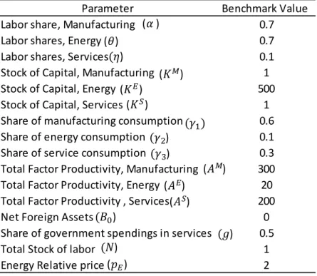
Table 1. Parameters Values
The model benchmark parameters are given in table 1. The economy uses one where energy and manufacturing has the same output elasticity of labor. The aim of the parameters chosen below is to replicate an economy where the energy sector has a positive trade balance, while the manufacturing sector has a negative trade balance. These are characteristics of an economy like Angola, in which the main export goods are
of mineral kind. Given the simplicity of the model, and the assumption that = does
not allow to have at the same time a positive trade balance for energy and making this sector the main production sector with lower labor (the energy sector employees only
Parameter Benchmark Value Labor share, Manufacturing 0.7
Labor shares, Energy 0.7
Labor shares, Services 0.1
Stock of Capital, Manufacturing 1
Stock of Capital, Energy 500
Stock of Capital, Services 1
Share of manufacturing consumption 0.6 Share of energy consumption 0.1 Share of service consumption 0.3 Total Factor Productivity, Manufacturing 300 Total Factor Productivity, Energy 20 Total Factor Productivity , Services 200
Net Foreign Assets 0
Share of government spendings in services 0.5
Total Stock of labor 1
Energy Relative price 2
( ) ( ) ( ) ( ) ( ) ( ) ( ) ( ) ( ) ( ) ( ) ( ) ( ) ( ) ( ) ( )
28
about 1% of the workforce in Angola). This is due the fact that to increase the production it is necessary to increase the labor or the capital in that sector and this will always lead to higher labor in energy, while the labor in manufacturing decreases.
In that sense a calibration is used with a benchmark where the manufacturing sector employs more labor than the energy and the non-tradable sector, replicates partially the conditions of Angola’s economy. Nevertheless, the results are still robust and allow extending the findings of Section 5. Given these values to the parameters, the benchmark scenario is given in table 2.
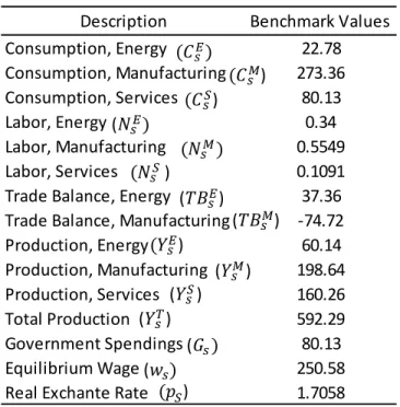
Table 2. Simulation 1: Benchmark
As stated before total labor is set to unit, and the net assets are set to zero. This assumption allows having an economy where the manufacturing is the more productive sector, where labor employed in the sector is about 55%. The aim of this calibration is to have an energy sector that is a net exporter while the manufacturing sector is a net importer, and so replicating a country that is a net exporter of energy.
Description Benchmark Values Consumption, Energy 22.78 Consumption, Manufacturing 273.36 Consumption, Services 80.13 Labor, Energy 0.34 Labor, Manufacturing 0.5549 Labor, Services 0.1091
Trade Balance, Energy 37.36 Trade Balance, Manufacturing -74.72 Production, Energy 60.14 Production, Manufacturing 198.64 Production, Services 160.26 Total Production 592.29 Government Spendings 80.13 Equilibrium Wage 250.58
Real Exchante Rate 1.7058 ( ) ( ) ( ) ( ) ( ) ( ) ( ) ( ) ( ) ( ) ( ) ( ) ( ) ( ) ( )
29
6.2 Main Results
This section will present the effects in the equilibrium of permanent shocks in exogenous variables mainly to assess the effects in labor allocation. All the shocks are related to 20% change in the studied variable.
6.2.1 Improvement in TFP Energy Sector
In this section a change in TFP of energy is analyzed, keeping everything else constant. The results are shown in the table (3) below.
Table 3. Simulation 2: Change in Energy TFP
Changing energy’s TFP from 20 to 24 leads to an increase of marginal productivity of labor, which means higher wages, which increase 8.6%, leading workers to move from the manufacturing sector to the energy sector, decreasing the production in the former and increasing in the latter. The total production in the energy sector increases about 52% while the production in manufacturing decreases about 17%. In the model there is no impact in production, or consumption, of services, due to a real appreciation that offsets the effects related to the improvement of TFP on energy by equalizing the wages of the non-tradable to the tradable, and so avoiding labor to move out of the sector. Given that
Description Benchmark Values Change in Energy TFP Consumption, Energy 22.78 24.733 Consumption, Manufacturing 273.36 296.80 Consumption, Services 80.13 80.125 Labor, Energy 0.34 0.469 Labor, Manufacturing 0.5549 0.422 Labor, Services 0.1091 0.109
Trade Balance, Energy 37.36 66.417 Trade Balance, Manufacturing -74.72 -132.84
Production, Energy 60.14 91.15 Production, Manufacturing 198.64 163.96 Production, Services 160.26 160.26 Total Production 592.29 643.06 Government Spendings 80.13 80.125 Equilibrium Wage 250.58 272.06
Real Exchante Rate 1.7058 1.852
( ) ( ) ( ) ( ) ( ) ( ) ( ) ( ) ( ) ( ) ( ) ( ) ( ) ( ) ( )
30
the increase in energy TFP causes an income effect, translated in higher real wages, the demand for goods increases the consumption for all goods, except for services. There is also a positive effect on the trade balance of energy, since the increase in production is higher than the consumption. In the case of manufacturing goods, the increase in demand to be satisfied partially by higher imports that cover the decrease in production in this sector. The overall effect of the improvement in the energy TFP is a higher national welfare, given the higher overall consumption, despite the decrease in the manufacturing sector (the de-industrialization).
6.2.2 Increase in energy prices
In this section a change in the energy relative price is analyzed, and the results are presented in table 4. The result of this shock to labor allocation was already presented in proposition 4, and now it is mainly intended to check the effects to consumption of energy which was not possible to assess in the proposition.
Table 4. Simulation 3: Change in Energy Relative Prices
Description Benchmark Values Change in Energy Relative Prices Consumption, Energy 22.78 20.611 Consumption, Manufacturing 273.36 296.80 Consumption, Services 80.13 80.125 Labor, Energy 0.34 0.469 Labor, Manufacturing 0.5549 0.422 Labor, Services 0.1091 0.109
Trade Balance, Energy 37.36 55.348
Trade Balance, Manufacturing -74.72 -132.84
Production, Energy 60.14 75.959 Production, Manufacturing 198.64 163.96 Production, Services 160.26 160.26 Total Production 592.29 643.06 Government Spendings 80.13 80.125 Equilibrium Wage 250.58 272.06
Real Exchante Rate 1.7058 1.852
( ) ( ) ( ) ( ) ( ) ( ) ( ) ( ) ( ) ( ) ( ) ( ) ( ) ( ) ( )