COMBINED FIELD/MODELLING APPROACHES TO REPRESENT
1
THE AIR-VEGETATION DISTRIBUTION OF BENZO[a]PYRENE
2
USING DIFFERENT VEGETATION SPECIES
3
Nuno Ratola* and Pedro Jiménez-Guerrero 4
Physics of the Earth, Regional Campus of International Excellence “Campus Mare 5
Nostrum”, University of Murcia, Edificio CIOyN, Campus de Espinardo, 30100 Murcia, 6
Spain 7
8
*Tel: +34 86888 8552; e-mail: [email protected]
9 10
Abstract
11
A strategy designed to combine the features of field-based experiments and modelling 12
approaches is presented in this work to assess air-vegetation distribution of benzo(a)pyrene 13
(BaP) in the Iberian Peninsula (IP). Given the lack of simultaneous data in both 14
environmental matrices, a methodology with two main steps was employed. First, evaluating 15
the simulations with the chemistry transport model (CTM) WRF (Weather Research and 16
Forecasting) + CHIMERE data against the European Monitoring and Evaluation Programme 17
(EMEP) network, to test the aptitude of the CTM to replicate the respective atmospheric 18
levels. Then,, using modelled concentrations and a method to estimate air levels of BaP from 19
biomonitoring data to compare the performance of different pine species (P. pinea, P. 20
pinaster, P. nigra and P. halepensis) to describe the atmospheric evidences.The comparison 21
of modelling vs. biomonitoring has a higher dependence on the location of the sampling 22
points, rather than on the pine species, as some tend to overestimate and others to 23
underestimate BaP concentrations, in most cases regardless of the season. The climatology of 24
the canopy levels of BaP was successfully validated with the concentrations in pine needles 25
(most biases below 26%), however, the model was unable to distinguish between species. 26
This article was published in Atmospheric Environment, 106, 34-42, 2015 http://dx.doi.org/10.1016/j.atmosenv.2015.01.063
especially in summer and autumn, the. The comparison with biomonitoring data showed a 28
similar pattern, but with the best results in the warmer months. 29
30
Keywords: Benzo(a)pyrene; Pine needles; biomonitoring; air sampling; WRF+CHIMERE;
31 32
1. Introduction
33 34
Polycyclic aromatic hydrocarbons (PAHs) are atmospheric pollutants originated from 35
several natural (forest fires, volcanoes) and anthropogenic (traffic, industry) sources, via the 36
combustion of fossil fuels, wood or other organic materials. But their release into the 37
environment as a consequence of human activities is increasing continuously (Lapviboonsuk 38
and Loganathan, 2007). The noticeable differences in their physical-chemical properties have 39
a decisive influence on their emission, transport and deposition behaviour (Ravindra et al., 40
2008). Both gaseous and particulate PAHs can undergo atmospheric transport over long 41
distances (Baek et al., 1991), carrying potentially high toxicity towards organisms worldwide 42
(Solé, 2000). 43
Several chemistry transport model (CTM) approaches tried to describe the levels and 44
patterns of PAHs (Sehili and Lammel, 2007; Matthias et al., 2009; Bieser et al., 2012; 45
Friedman and Selin, 2012; San José et al., 2013). In particular benzo(a)pyrene (BaP), 46
predominantly found in the particulate fraction of the atmosphere and the reference for the 47
existing air quality standards for PAHs (European Commission, 2008). However, CTMs still 48
cannot provide a full understanding of the processes involved in their atmospheric fate 49
(Galarneau et al., 2013), being the lack of field data reporting atmospheric concentrations a 50
major reason for this fact. For instance, the measuring stations of the European Monitoring 51
and Evaluation Programme (EMEP) network cover the whole European territory, but those 52
monitoring semi-volatile organic compounds (SVOCs) like PAHs are located essentially in 53
the Scandinavian countries and almost absent from the southern European countries (Bieser 54
et al., 2012; Torseth et al., 2012). This is why the use of alternative ways to include field 55
sampling data in the validation of the models has to be considered. 56
One valid option is performing monitoring studies employing vegetation species, which 57
have been used for some time in the assessment of PAHs levels. Coniferous species, in 58
particular the lipid-rich cuticle of their needles, is likely to accumulate such contaminants 59
(Simonich and Hites, 1995) and are favoured due to their ubiquity, which allows the 60
establishment of trans-boundary studies (Lehndorff and Schwark, 2004). According to 61
McLachlan (1999), PAHs can reach the needles by equilibrium partitioning between the 62
vegetation and the gas phase, kinetically-limited gaseous deposition, or wet and dry particle-63
bound deposition. A few studies proved the ability of coniferous needles to establish levels 64
and spatio-temporal patterns of PAHs (Lehndorff and Schwark, 2009; Augusto et al., 2010; 65
Ratola et al., 2010a, 2010b, 2012; Amigo et al., 2011), but only a very limited number of 66
literature is available regarding the air-vegetation distribution, in controlled systems (Zhu et 67
al, 2008) or in field-based studies (St Amand et al., 2009a, 2009b). However, the strong 68
potential of biomonitoring data and CTMs can be used in concomitance to obtain reliable 69
estimates of the air-vegetation partition of PAHs. Differences between the uptake capacity of 70
the needles of several pine species and the dissimilar levels depending on the land use have 71
been reported in biomonitoring schemes (Librando et al., 2002; Piccardo et al., 2005; Ratola 72
et al, 2011), and it would be very important that CTMs could represent those differences 73
adequately, especially in areas where data regarding persistent atmospheric pollutants is 74
scarce, such as the western Mediterranean (Bernalte et al., 2012). 75
As such, an innovative approach using the Weather Research and Forecasting 76
(WRF)+CHIMERE modelling system, coupled to emission data from EMEP and compared 77
to data from 70 pine needles sampling sites is presented in this work. The main objective is to 78
evaluate the presence of BaP in the Iberian Peninsula, in order to verify if models and field 79
data can represent accurately their atmospheric concentrations, and at the same time unveil 80
possible differences between pine species (in this case Pinus pinea, Pinus pinaster, Pinus 81
nigra and Pinus halepensis).
82 83
2. Experimental Section
84 85
2.1. Pine needles sampling and analysis 86
Details on the sampling campaigns taken in consideration for the pine needles can be 87
found elsewhere (Ratola et al., 2010a; 2012). A brief description can be found in Supporting 88
Information. 89
90
2.2. Estimation of BaP air concentrations from pine needles 91
An estimation of atmospheric concentrations of BaP in the sampling sites chosen for this 92
study was performed using the levels found in pine needles. This indirect calculation was 93
necessary to face the scarce information on the atmospheric presence of BaP in the area of 94
study. The methodology employed is based on the studies by St. Amand et al. (2007, 2009a, 95
2009b), who determined levels of gas-phase and particulate PAHs (and PBDEs) in vegetation 96
and in the nearby atmosphere. They reported an approach to estimate the air concentrations 97
from those found in vegetation, consisting briefly in the following calculations: 98
Ca = Cp + Cg (eq. 1) with 99
Cp = (Cvp*m) / (A*vp*t) (eq. 2) and
100
Cg = (Cvg*m) / (A*vgt*t) (eq. 3)
101
where Ca, Cp, Cg – total, particulate and gas-phase (respectively) concentrations of the target 102
compound in air (ng m-3); Cvp, Cvg - contribution of particle-bound and gaseous deposition
103
(respectively) to the total concentration in vegetation (defined as Cvp+Cvg, ng g-1); m - dry
104
weight of pine needles (g); A - total surface area of pine needles (m2); v
p - particle-bound
deposition velocity (m h-1); v
gt - net gaseous transfer velocity (m h-1); t - environmental
106
exposure time of pine needles (h). For BaP, the gas-phase contribution is strongly 107
predominant (ASTDR, 1995; Friedman and Selin, 2012), so the gas-phase contribution is 108
considered negligible (St. Amand et al., 2009a), meaning Cg ≈ 0 and Ca ≈ Cp. This way, vp
109
can be calculated by equation 2, if the concentrations in air (Ca) and vegetation (Cvp) are 110
known. However, due to the lack of atmospheric measurements, it was impossible to 111
calculate vp for our samples. So, given that the value reached by St. Amand et al. (2009a)
112
was for Norway spruce (Picea abies) needles, it was decided to use the deposition velocity 113
estimated for BaP over a coniferous forest canopy by Horstmann and McLachlan (1998): 114
2.196 m h-1. This way, it is possible that the differences in the PAHs uptake by different pine
115
species found in literature (Librando et al., 2002; Piccardo et al., 2005; Ratola et al., 2011) 116
were somehow compensated in this first approximation. Table S1 (Supporting Information) 117
presents the mass and total surface area for the pine needles species considered in this work. 118
The exposure time (in hours) was estimated from April 15th (considered as the day the
119
needles sprung out) to the sampling day. 120
121
2.3. Modelling experiment 122
In this study, the modelling system consists on the Advanced Research Weather Research 123
and Forecasting (WRF-ARW) Model v3.1.1 (Klemp et al., 2007; Skamarock et al., 2008) 124
coupled off-line to the CHIMERE chemistry transport model (Menut et al., 2013). Details are 125
presented in Supporting Information. 126
127
2.4. Model evaluation 128
For the evaluation of canopy deposition and atmospheric concentrations, the spatial 129
correlation coefficient (r), root mean square error (RMSE) and mean bias (MB) values were 130
selected after Pay et al. (2010). Annual and seasonal mean statistics are computed, with 131
seasons corresponding to December, January and February (DJF, winter), March, April and 132
May (MAM, spring), June, July and August (JJA, summer) and September, October and 133
November (SON, autumn). Also, the mean fractional bias (MFB) and the mean fractional 134
error (MFE) will be used instead of the mean normalised bias error (MNBE), since Boylan 135
and Russell (2006) reported that the latter may not be appropriate for evaluating particulate 136
materials. This is due to the fact that the concentrations of these components can be 137
considerably low, leading sometimes to very large normalised biases and errors when 138
observations are close to zero, even though the absolute biases and errors are very small. 139
These authors defined a performance goal (both MFE and MFB are less than or equal to 50% 140
and ±30%, respectively) and a model performance criterion (MFE ≤ 75% and MFB ≤ ±60%) 141
to be met by the errors obtained. 142
Results from the field-based air monitoring made within EMEP were used to characterise 143
the ability of the model to reproduce present air BaP levels and variability. EMEP stations 144
are located at a minimum distance of approximately 10 km from large emission sources and 145
thus assumed to fit the resolution of the model used for regional background concentrations 146
(Torseth et al., 2012). Although the collection and analysis of the pine needles covered the 147
period of late 2006-2007, the data available from EMEP stations in the Iberian Peninsula 148
regarding the levels of BaP was scarce, so it was decided to extend the EMEP data range to 149
2006-2010, in order to have statistically representative results and enhanced reliability of the 150
model validation. 151
As one of our aims is to have the best approximation of atmospheric BaP levels through 152
modelling procedures, the multiplicative ratio bias-correction technique was applied 153
following the methodology of Borrego et al. (2011) and Monteiro et al. (2013). A four-week 154
training period was chosen here as a compromise of having a sufficiently long timeframe to 155
gather adequate statistics but not as much as to mask seasonal variations. 156
157
3. Results and Discussion
158 159
3.1. Description of model climatologies 160
Since this work focuses on the climatologies (values of a variable which is significant for 161
a certain period of time and also climatologically representative) of the BaP levels canopies 162
and in the air over the Iberian Peninsula, first the estimations made by the modelling system 163
used are presented. 164
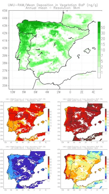
Figure 1 indicates the total annual deposition on vegetal canopies and the seasonal 165
contribution to annual deposition as represented by WRF+CHIMERE. Areas with a larger 166
deposition are coincident with most vegetated areas of the Iberian Peninsula (Figure S1, 167
Supporting Information), so the growing cycle of the different species can have a strong 168
influence on the canopy levels, together with the emissions of pollutants. Hence, differences 169
in the entrapment of PAHs by the different land uses may play a significant role, as observed 170
in the spatial pattern of uptake. The largest annual deposition amounts are about 50 ng g-1 in
171
northern and north-western areas, while non-vegetated areas obviously present negligible 172
depositions (northern and central plateaus, Guadalquivir and Guadiana river valleys in the 173
south or Ebro valley in the north-east). In terms of levels, the contribution to the deposition 174
values of BaP is lowest for JJA (under 5% over most of the Iberian Peninsula, except in 175
Portugal and northern Spain, with 5% to 10%) and have the highest values in DJF and 176
especially in MAM (when the contribution is over 30-40% for the entire Iberian Peninsula 177
except in the northern Atlantic coast, where it ranges from 20 to 30%, see Figure 1). 178
Apparently, although the levels of BaP over the canopy seem to follow the density of 179
vegetation, it is clear that the seasonal patterns are in line with the commonly described 180
variations of the BaP content in the atmosphere (Prevedouros et al., 2004; Garrido et al., 181
2014). 182
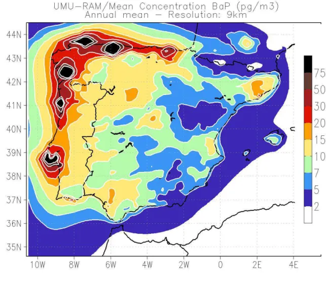
Regarding the atmosphere, the BaP concentrations obtained by the model for the period 183
2006-2010 (Figure 2) indicate the highest incidences surpassing in some cases 75 pg m-3
184
(NW Spain and western coast of Portugal), although the levels in background areas hardly 185
exceed 5 pg m-3 (lowest incidence in the SE Levantine coast). Although the highest BaP
186
concentrations in the atmosphere are mainly found in urban and industrial settings, that is, 187
near the predominant emitting sources (Jaward et al., 2004), this is only partially seen in the 188
current results. In fact, in the north and west Iberian Peninsula, the major urban and industrial 189
areas such as Lisbon, Porto, A Coruña or Santander show the highest levels (Figure 2). But 190
for the main urban conurbations in all Iberia (Madrid and Barcelona), the model estimates 191
lower BaP concentrations comparatively, but still higher than the mean values in the 192
east/centre/south of the domain. The reasons can be several, including different types of fuel 193
that can be used in house heating or industrial processes in areas with different climatic 194
patterns. In any case, only the validation of these model estimations with field data can 195
clarify if this spatial fingerprint is accurate. 196
197
3.2. Model validation 198
199
3.2.1. BaP canopy estimations 200
The accuracy of pine needles to reflect the incidence of semi-volatile organic 201
contaminants in general is described in literature (Eriksson et al., 1989; Klánová et al., 2009). 202
Gas and particulate phase cannot be distinguished, and the former tend to be better captured 203
by the waxy layer of the needles. In the case of BaP the gas-phase content is negligible, as 204
mentioned previously, so there is no effect of partition between the two phases and the air-205
vegetation calculations can be more reliable (Chun, 2011). The field-based BaP 206
concentrations used in this work to validate the canopy estimations of the modelling system 207
are taken from monitoring campaigns previously performed in the Iberian Peninsula using 208
pine needles (Ratola et al., 2009, 2010a, 2012). These data were compared to the deposition 209
over vegetal canopies estimated by the CHIMERE transport model. The results were divided 210
by each of the four pine species monitored, in order to assess the potential differences 211
between them regarding the validation of the model. 212
Hence, the model validation parameters for canopy deposition are summarised in Table 1, 213
revealing an overall good performance of the model to reproduce the uptake of BaP by 214
vegetation was observed, when compared to the results in pine needles. In fact, a general 215
view indicates that the model tends to overpredict the BaP concentrations in pine needles 216
during DJF and MAM and underpredicts them for JJA (no conclusion can be obtained for 217
SON). The root mean-square error (RMSE) remains under 2 ng g-1 in all seasons and species,
218
indicating a close link of the model to the levels obtained from pine needles. The accurate 219
representation of the temporal patterns over the Iberian Peninsula (over 0.7 for P. pinea and 220
P. pinaster, see Table 1) is worthy of mention, indicating that despite the model bias, the
221
time reproducibility of the deposition patterns over the Iberian Peninsula captures accurately 222
the seasonal distribution. In fact, some authors report that the concentrations of these classes 223
of contaminants in pine needles are more influenced by biological processes than the air 224
concentrations (Kylin and Hellstrom, 2003). Nevertheless, the seasonal fingerprints are 225
clearly present in this case. 226
Considering all samples analyzed regardless of location, it is interesting to focus first on 227
the seasons with largest climatic differences over the Iberian Peninsula: winter (DJF) and 228
summer (JJA). The mean BaP concentration shown by the P. pinea needles in DJF (1.25 ± 229
0.84 ng g-1) is significantly lower than for P. pinaster needles (2.70 ± 2.40 ng g-1), as also
230
reported by Ratola et al. (2011). This is in addition confirmed by the CTM deposition 231
concentrations, exhibiting values of 1.51 ± 1.41 ng g-1 and 3.14 ± 2.20 ng g-1 for P. pinea and
232
P. pinaster, respectively. For JJA, this behaviour is analogous, showing P. pinaster the
233
highest measured and modelled values (1.40 ± 0.89 ng g-1 and 1.08 ± 0.77 ng g-1,
234
respectively). For P. pinea during the summer season, the pine needles indicate a mean 235
concentration of 1.15 ± 0.91 ng g-1, while the model reproduces depositions of 0.69 ± 0.49 ng
236
g-1. It is noticeable that for both pine species the model tends to overpredict the DJF
237
depositions (bias = 0.26 ng g-1 for P. pinea and 0.44 ng g-1 for P. pinaster; with respective
238
MFB = 6.76% and 23.82%), while in JJA the behaviour is opposite, with a slight trend to 239
underestimate the measured concentrations (bias = -0.46 ng g-1 for P. pinea and -0.32 ng g-1
240
for P. pinaster; MFB = -47.65% and -25.89%, in that order). The summer underestimation 241
may be caused by the tendency of the model to volatilise SVOCs as a result of the high 242
temperatures simulated with the model over the Iberian Peninsula. 243
The aforementioned results are consistent with the work of Piccardo et al. (2005) or 244
Ratola et al. (2011), who showed that P. pinaster needles have a superior uptake capacity 245
towards PAHs than P. pinea or P. nigra. The former two species are two of the most 246
predominant in the forests of the Iberian Peninsula, but while P. pinea is more equally 247
distributed although mainly present in the south and Mediterranean coast, P. pinaster prevails 248
in the north-west and Atlantic coast. It was also suggested that leaf surface properties are 249
more a function of the environmental exposure than of the plant response (Cape et al., 1989). 250
Given all these facts, the models face a huge task to represent the levels of pollutants in 251
vegetation. 252
An important finding arises from the comparison between pine species. Considering the 253
sites where it was possible to collect needles from two contiguous trees (Antuã and Quintãs, 254
coordinates 40.6949N 8.5225W; 40.5758N 8.6294W), with P. pinaster and P. pinea, it is 255
clear that they presented dissimilar BaP entrapment abilities, with concentrations in Antuã of 256
3.75 ng g-1 and 2.71 ng g-1 (for P. pinaster and P. pinea, respectively) and 2.07 ng g-1 (0.74
257
ng g-1) for P. pinaster (P. pinea) in Quintãs, as annual mean concentrations. This is in line
258
with the studies of Ratola et al. (2010a), who stated that P. pinaster needles have overall 259
stronger adsorption ability towards the sum of the 16 EPA (U.S. Environmental Protection 260
Agency) PAHs, and most PAHs individually (including BaP). 261
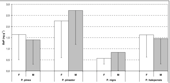
However, the inability of the model to distinguish between pine species can be inferred 262
from Figure 3, where all the data from field campaigns (F) and modelling (M) available was 263
combined and averaged. The CTM tends to underpredict the concentrations over P. pinaster 264
and overestimate the depositions over P. pinea (Figure 3). This is due to the assumptions in 265
the deposition velocity made by the model (which considers the several vegetation species as 266
a whole canopy). Although the discussion is brought by the simultaneous sampling of P. 267
pinaster and P. pinea, it can also be seen that for the other two pine species sampled (P.
268
nigra and P. halepensis, only available for SON), the same intermediate behaviour can be
269
observed in the model validation parameters (overestimation for P. nigra, bias = 0.27 ng g-1
270
and MFB = 5.74%; underestimation for P. halepensis, bias = -0.17 ng g-1 and MFB =
-271
17.30%, see Table 1) and the global field/model comparison (Figure 3). 272
The model representation of uptake and partition processes of organic contaminants into 273
vegetation is, by itself, challenging (Barber et al., 2004). The gaps still existing in the 274
understanding of these phenomena reflects on the ability to reproduce the interactions with 275
the atmospheric loads as well. Both field-based and computational approaches have been 276
improved along the years, trying to take into account increasingly more crucial aspects that 277
influence the behaviour of the pollutants, such as meteorological parameters (Klánova et al., 278
2008; Jiménez-Guerrero et al., 2008). The easiest approach is, naturally, to consider 279
vegetation as a big canopy, as did, for instance, Horstmann and McLachlan (1998), since it 280
would be impossible on a large scale to distinguish between every species present. But what 281
the results of this work show is that models may be able to incorporate a particular species or 282
some of them with not such a big effort in the future. 283
284
3.2.2. BaP air estimations 285
For air levels, a validation against EMEP field-based air quality data after the removal of 286
the bias is required, to assess the correct reproducibility of the spatial-temporal patterns of 287
BaP by WRF+CHIMERE. As mentioned previously, studies in literature regarding the field 288
monitoring of levels of PAHs in the Iberian Peninsula are scarce and, therefore, modelling 289
strategies can represent a valuable tool for assessing BaP levels over the target region. As 290
seen in Table S2 (Supporting Information), the atmospheric concentrations of BaP modelled 291
present mean fractional errors (MFE) under 25% over all the EMEP stations in the Iberian 292
Peninsula, except in the case of Peñausende station (ES0013R), where MFB=+43%. Annual 293
mean concentrations of BaP in air show both positive and negative mean fractional biases 294
(MFB), depending on the stations. This fact indicates that the model does not fall 295
predominantly towards overprediction or underpredicion for the area in question, with 296
deviations (Table S3, Supporting Information) from +1.63 pg m-3 in Peñausende station and
-297
4.59 pg m-3 in San Pablo de los Montes. These low values confirm that the model estimates
298
can be used as a reference for the comparison with the levels of atmospheric concentrations 299
of BaP obtained from air-vegetation estimation calculations. 300
301
3.3. Atmospheric levels using biomonitoring data 302
Given that the model represents accurately the air concentrations of BaP, in this section 304
the modelled concentrations were considered as a pseudo-reality (a low-biased simulation 305
that was tested to accurately reproduce reality at observation points and therefore can be used 306
as a physico-chemical consistent reality, despite the obvious errors associated to modelling 307
techniques) to act as a reference to validate the approach employed to convert vegetation 308
levels into atmospheric concentrations. Biomonitoring campaigns can produce helpful 309
datasets to compensate the current scarcity of information on the atmospheric presence of 310
PAHs (and other pollutants of high concern) over the Iberian Peninsula. So, profiting from 311
pine needles sampling studies conducted in this region, an estimation of the BaP 312
concentrations in the atmosphere of each sampling point was done, since the loads in pine 313
needles have an atmospheric source (Hwang and Wade, 2008). An approach developed by St. 314
Amand and co-workers (2007, 2009a, 2009b) was used for this purpose, taking in 315
consideration the deposition velocity of BaP found by Horstmann and McLachlan (1998) 316
over a coniferous forest canopy. The validation of the model can take advantage from this 317
approach, matching the air concentrations found to those of the pseudo-reality given by the 318
CTM. 319
Results are presented in Table 2 and show that the BaP concentrations are generally 320
higher in the coldest season (winter). This is expected and has been reported previously 321
(Lehndorff and Schwark, 2009), since winter triggers an increase of PAH sources, namely 322
domestic heating and heavier road traffic. Over P. pinea sampling sites, modelled 323
concentrations (considered in this case as the pseudo-reality) for DJF are 13.29±13.22 pg m-3,
324
showing very similar values to the samples collected over P. pinaster sites (15.28±14.53 pg 325
m-3). However, the air estimates from vegetation done according to the methodology based
326
on St. Amand et al. (2007, 2009a, 2009b) and explained in section 2.2, reveal a larger 327
disagreement: while estimations over P. pinea sites indicate a mean concentration of 328
8.70±5.88 pg m-3 (and therefore clearly underestimating the winter concentrations as
329
reproduced by the CTM), the approach for P. pinaster data largely overestimates the pseudo-330
reality reproduced by the model (28.43±23.78 pg m-3). This general behaviour is observed for
331
the mean values on Figure 2. A similar trend is observed for summer, where the air-332
vegetation approach underestimates the atmospheric concentrations when using P. pinea 333
data, but overestimates for P. pinaster. The ratios between winter/summer concentrations are 334
2.43 (1.74) over P. pinea sampling sites for the CTM (air-vegetation approach) and 2.00 335
(3.22) when using P. pinaster needles. The importance of the species is therefore noticeable 336
when trying to reproduce the temporal patterns using the air-vegetation approach. A possible 337
explanation for these differences can be found in Hwang and Wade (2008) and Ratola et al. 338
(2010b), who demonstrated the variability of PAHs uptake by needles of different pine 339
species and for different seasons. As reported by those authors, this is much more visible in 340
the lighter PAHs (the ones in the gas-phase), given their stronger affinity to the pine needles 341
lipidic cuticle, if compared to particulate PAHs such as BaP. The concentrations of the latter 342
may not suffer as strong seasonal variation in pine needles as that conveyed by the different 343
emission rates from winter to summer. The seasonal results presented here agree with the 344
work of Menichini (1992), who reported that the levels of atmospheric PAHs are 2 to 10 345
times higher in the colder months. Moreover, the air temperature dependence can also 346
suggest that increased partitioning in the winter fuelled a higher accumulation of BaP in pine 347
needles (Hwang and Wade, 2008). An enhanced volatilisation in warmer periods would also 348
contribute towards a lower BaP incidence. 349
Comparing the mean atmospheric concentrations estimated by the CTM modelling (M) 350
and the air-vegetation conversion (S) by using the St. Amand et al (2007, 2009a, 2009b) 351
approach, described in section 2.2 (Figure 4), only the P. halepensis results are identical for 352
the modelling and conversion methods, while there is a significant difference for P. nigra 353
needles. For P. pinea and P. pinaster the trends are opposite, so there is no clear indication of 354
a consistent behaviour of such comparisons in terms of mean atmospheric incidence. 355
Interestingly, results indicate that none of the pine species considered in the current study 356
outperforms the others when reproducing the pseudo-reality provided by the model (Table 2). 357
For DJF, the MFB ranges from the underestimation (-43.26%) for P. pinea to an 358
overestimation using P. pinaster (+49.60%). Despite the different sign, the relative 359
magnitude of these errors is analogous. A similar behaviour is observed for JJA (MFB of -360
28.46% when using P. pinea vs. +28.78% for P. pinaster). These errors can be considered as 361
acceptable, bearing in mind the diversity of the sampling sites considered in this work and 362
the model performance criterion established by Boylan and Russell (2006) (MFB ≤ ±60%). 363
The lowest fractional biases are found for P. halepensis (+8.94%), while the only value 364
exceeding the MFB performance criterion is found for P. nigra (-67.86%). Again, both 365
species were only accountable for the autumn (SON) season. 366
With respect to the temporal correlation coefficients, comparable results are found for 367
each pine species with available data (r>0.7), and only small differences are found (0.73 for 368
P. pinea and 0.70 for P. pinaster), displaying an adequate description of the temporal
369
variability observed using all sampling data. Even if the actual concentrations are not very 370
well described, the temporal air-needles synergies are accurately projected by this approach. 371
The spatial correlation coefficients (which provide a simulation for the adequate 372
representation of the BaP spatial patterns over the Iberian Peninsula) are, in general, correctly 373
reproduced by the air-vegetation approach (Table 2). The highest value is seen for summer in 374
the case of P. pinaster and for autumn when estimating air concentrations from P. pinea 375
(r=0.93). Both species also reproduce the modelled spatial patterns of BaP during spring 376
(r>0.8). Conversely, the lowest spatial correlation coefficients (under 0.5) are found for 377
summer/P. pinea, autumn/P. pinaster and autumn/P. halepensis. There is no apparent reason 378
for this evidence other that some particular characteristics of the pine species and the 379
sampling sites associated to them. 380
Being the basis of the field data input an estimation of the atmospheric concentrations 381
from the levels in pine needles, it can be suggested that the deposition velocity chosen may 382
not be the best for our domain, but instead the one closer to the approximation of the 383
deposition over vegetal canopies included in the model. However, as the results were 384
validated over an extended time frame (2006-2010) with BaP field concentrations given by 385
EMEP stations with very good results (as mentioned previously), proving that the model 386
estimates are matching positively the conditions of the area. 387
388
4. Conclusions
389 390
The current study has shown the ability of pine needles to act as biomonitors of BaP 391
atmospheric levels when coupled with CTM strategies, regardless of the species used in the 392
assessment. The validation of WRF+CHIMERE (+EMEP emissions) simulations against the 393
data available from the EMEP network was done to verify the skills of the CTM to reproduce 394
BaP levels over the Iberian Peninsula, before employing the modelled concentrations as a 395
pseudo-reality to compare with a vegetation-air estimating approach applied to four pine 396
species (P. pinea, P. pinaster, P. nigra and P. halepensis). 397
The WRF+CHIMERE method was found to mimic accurately the atmospheric 398
concentrations of BaP and their spatial and temporal patterns over vegetation in the Iberian 399
Peninsula, as was the approach based on the work of St. Amand and co-workers to estimate 400
air concentrations from pine needles levels considered a good alternative to overcome the 401
lack of information on the atmospheric presence of BaP in Iberia. In this line, other pollutants 402
with even less or no data at all can be considered using a similar set-up.. 403
Moreover, the results found reinforce the idea that the modelling results depend more 404
strongly on the location of the pine species collected (for evaluation purposes) than on the 405
pine species themselves, since the model presents an intermediate behaviour. However, 406
research on these matters should be significantly enhanced, particularly in the ability of the 407
models to identify and reproduce different vegetation species, which in turn can help in the 408
design of biomonitoring field campaigns. Namely, choosing which species is the most 409
appropriate for the study in question among the available ones. 410
411
Acknowledgements
412
This work was partially funded by the European Union Seventh Framework Programme-413
Marie Curie COFUND (FP7/2007-2013) under UMU Incoming Mobility Programme 414
ACTion (U-IMPACT) Grant Agreement 267143. The Spanish Ministry of Economy and 415
Competitiveness and the "Fondo Europeo de Desarrollo Regional" (FEDER) (project 416
CORWES CGL2010-22158-C02-02) are acknowledged for their partial funded. Dr. Pedro 417
Jiménez-Guerrero acknowledges the Ramón y Cajal programme. 418
419
Appendix A. Supplementary data
420
Supplementary data related to this article can be found at… 421
422
References
423
Amigo, J.M., Ratola, N., Alves, A., 2011. Study of geographical trends of polycyclic 424
aromatic hydrocarbons using pine needles. Atmospheric Environment 45, 5988-5996. 425
Agency for Toxic Substances and Disease Registry (ATSDR), 1995. Toxicological profile 426
for polycyclic aromatic hydrocarbons. ATDSR, August 1995, Atlanta, GA. 427
Augusto, S., Máguas, C., Matos, J., Pereira, M. J., Branquinho, C. 2010. Lichens as an 428
integrating tool for monitoring PAH atmospheric deposition: A comparison with soil 429
air and pine needles. Environmental Pollution 158, 483–489. 430
Baek, S.O., Field, R.A., Goldstone, M.E., Kirk, P.W., Lester, J.N., Perry, R., 1991. A review 431
of atmospheric polycyclic aromatic hydrocarbons: sources, fate and behaviour. Water, 432
Air and Soil Pollution 60, 279-300. 433
Barber, J.L., Thomas, G.O., Kerstiens, G., Jones, K.C., 2004. Current issues and uncertainties 434
in the measurement and modelling of air–vegetation exchange and within-plant 435
processing of POPs. Environmental Pollution 128, 99-138. 436
Bernalte, E., Marín-Sánchez, C., Pinilla-Gil, E., Cerceda-Balic, F., Vidal-Cortex, V., 2012. 437
An exploratory study of particulate PAHs in low-polluted urban and rural areas of 438
south-western Spain: concentrations, source assignment, seasonal variations and 439
correlations with other pollutants. Water, Air, and Soil Pollution 223, 5143-5154. 440
Bieser, J., Aulinger, A., Matthias, V., Quante, M., 2012. Impact of emission reductions 441
between 1980 and 2020 on atmospheric benzo[a]pyrene concentrations over Europe. 442
Water, Air, and Soil Pollution 223, 1391-1414. 443
Borrego, C., Monteiro, A., Pay, M.T., Ribeiro, I., Miranda, A.I., Basart, S., Baldasano, J.M., 444
2011. How bias-correction can improve air quality forecasts over Portugal. 445
Atmospheric Environment 45, 6629-6641. 446
Boylan, J.W., Russell, A.G., 2006. PM and light extinction model performance metrics, 447
goals, and criteria for three-dimensional air quality models. Atmospheric Environment 448
40, 4946–495 449
Cape, J.N., Paterson, I., Wolfenden, S.J., 1989. Regional variation in surface properties of 450
Norway spruce and Scots pine needles in relation to forest decline. Environmental 451
Pollution 58, 325-342. 452
Chun, M.Y., 2011. Relationship between PAHs concentrations in ambient air and deposited 453
on pine needles. Environmental Health and Toxicology 26, 6 p. 454
Eriksson, G., Jensen, S., Kylin, H., Strachan, W., 1989. The pine needle as a monitor of 455
atmospheric pollution. Nature 341, 42-44 456
European Commission, 2008. Directive 2008/50/EC of the European Parliament and of the 457
Council of 21 May 2008 on ambient air quality and cleaner air for Europe. Official 458
Journal of the European Union L 152, 1–44. 459
Friedman, C.L., Selin, N.E., 2012. Long-range atmospheric transport of polycyclic aromatic 460
hydrocarbons: a global 3-D model analysis including evaluation of Arctic sources. 461
Environmental Science and Technology 46, 9501–9510. 462
Galarneau, E., Makar, P.A., Zheng, Q., Narayan, J., Zhang, J., Moran, M.D., Bari, M.A., 463
Pathela, S., Chen, A., Chlumsky, R., 2013. PAH concentrations simulated with the 464
AURAMS-PAH chemical transport model over Canada and the USA, Atmospheric 465
Chemistry and Physics 13, 18417-18449. 466
Garrido, A., Jiménez-Guerrero, P., Ratola, N., 2014. Levels, trends and health concerns of 467
atmospheric PAHs in Europe. Atmospheric Environment 99, 474-484. 468
Horstmann, M., McLachlan, M.S., 1998. Atmospheric deposition of semivolatile organic 469
compounds to two forest canopies. Atmospheric Environment 32, 1799-1809. 470
Hwang, H.H., Wade, T.L., 2008. Aerial distribution, temperature-dependent seasonal 471
variation, and sources of polycyclic aromatic hydrocarbons in pine needles from the 472
Houston metropolitan area, Texas, USA. Journal of Environmental Science and Health 473
Part A 43, 1243-1251. 474
Jaward, F.M., Farrar, N.J., Harner, T., Sweetman, A.J., Jones, K.C., 2004. Passive air 475
sampling of polycyclic aromatic hydrocarbons and polychlorinated naphthalenes 476
across Europe. Environmental Toxicology and Chemistry 23, 1355–1364. 477
Jiménez-Guerrero, P., Jorba, O., Baldasano, J.M., Gassó, S., 2008. The use of a modelling 478
system as a tool for air quality management: annual high-resolution simulations and 479
evaluation. The Science of the Total Environment 390, 323-340. 480
Klánová, J., Čupr, P., Kohoutek, J., Harner, T., 2008. Assessing the influence of 481
meteorological parameters on the performance of polyurethane foam-based passive air 482
samplers. Environmental Science and Technology 42, 550-555. 483
Klánová, J., Čupr, P., Baráková, D., Šeda, Z., Anděl, P., Holoubek, I., 2009. Can pine 484
needles indicate trends in the air pollution levels at remote sites? Environmental 485
Pollution 157, 3248-3254. 486
Klemp, J.B., Skamarock, W.C., Dudhia, J., 2007. Conservative split-explicit time integration 487
methods for the compressible non-hydrostatic equations. Monthly Weather Review 488
135, 2987-1913. 489
Kylin, H., Hellstrom, A., 2003. Endogenous hydrophobic compounds affect the hydrophobic 490
capacity of plants and influence the forest filter effect. Stochastic Environmental 491
Research and Risk Assessment 17, 249–251. 492
Lapviboonsuk, J., Loganathan, B.G., 2007. Polynuclear aromatic hydrocarbons in sediments 493
and mussel tissue from the lowermost Tennessee River and Kentucky Lake. Journal of 494
the Kentucky Academy of Science 68,186-197. 495
Lehndorff, E., Schwark, L., 2004. Biomonitoring of air quality in the Cologne Conurbation 496
using pine needles as a passive sampler - part II: polycyclic aromatic hydrocarbons 497
(PAH). Atmospheric Environment 38, 3793-3808. 498
Lehndorff, E., Schwark, L., 2009. Biomonitoring airborne parent and alkylated three-ring 499
PAHs in the Greater Cologne Conurbation I: Temporal accumulation patterns. 500
Environmental Pollution 157, 1323-1331. 501
Librando, V., Perrini, G., Tomasello, M., 2002. Biomonitoring of atmospheric PAHs by 502
evergreen plants: correlations and applicability. Polycyclic Aromatic Compounds 22, 503
549–559. 504
Matthias, V., Aulinger, A., Quarte, M., 2009. CMAQ simulations of the benzo(a)pyrene 505
distribution over Europe for 2000 and 2001. Atmospheric Environment 43, 4078-4086. 506
McLachlan, M.S., 1999. Framework for the interpretation of measurements of SOCs in 507
plants. Environmental Science and Technology 33, 1799-1804. 508
Menichini, E., 1992. Urban air pollution by polycyclic aromatic hydrocarbons: levels and 509
sources of variability. The Science of the Total Environment 116, 109-135. 510
Menut, L., Bessagnet, B., Khvorostyanov, D., Beekmann, M., Blond, N., Colette, A., Coll, I., 511
Curci, G., Foret, G., Hodzic, A., Mailler, S., Meleux, F., Monge, J.L., Pison, I., Siour, 512
G., Turquety, S., Valari, M., Vautard, R., Vivanco, M.G., 2013. CHIMERE 2013: a 513
model for regional atmospheric composition modelling. Geoscientific Model 514
Development 6, 981-1028. 515
Monteiro, A., Ribeiro, I., Techepel, O., Sá, E., Ferreira, J., Carvalho, A., Martins, V., Strunk, 516
A., Galmarini, S., Elbern, H., Schaap, M., Builtjes, P., Miranda, A.I., Borrego, C., 517
2013. Bias correction techniques to improve air quality ensemble predictions: focus on 518
O3 and PM over Portugal. Environmental Modelling Assessment 18, 533-546.
519
Pay, M.T., Piot, M., Jorba, O., Gassó, S., Gonçalves, M., Basart, S., Dabdub, D., Jiménez-520
Guerrero, P., Baldasano, J.M., 2010. A full year evaluation of the CALIOPE-EU air 521
quality modeling system over Europe for 2004, Atmospheric Environment 44, 3322-522
3342. 523
Piccardo, M.T., Pala, M., Bonaccurso, B., Stella, A., Redaelli, A., Paola, G., Valério, F., 524
2005. Pinus nigra and Pinus pinaster needles as passive samplers of polycyclic 525
aromatic hydrocarbons. Environmental Pollution 133, 293-301. 526
Prevedouros, K., Brorström-Lundén, E., Halsall, C.J., Jones, K.C., Lee, R.G.M., Sweetman, 527
A.J., 2004. Seasonal and long-term trends in atmospheric PAH concentrations: 528
evidence and implications. Environmental Pollution 128, 17–27. 529
Ratola, N., Alves, A., Lacorte, S., Barceló, D., 2012. Distribution and sources of PAHs using 530
three pine species along the Ebro river. Environmental Monitoring and Assessment 531
184, 985-999. 532
Ratola, N., Amigo, J.M., Alves, A., 2010a. Comprehensive assessment of pine needles as 533
bioindicators of PAHs using multivariate analysis. The importance of temporal trends. 534
Chemosphere 81, 1517-1525. 535
Ratola, N., Amigo, J.M., Alves, A., 2010b. Levels and sources of PAHs in selected sites from 536
Portugal: biomonitoring with Pinus pinea and Pinus pinaster needles. Archives of 537
Environmental Contamination and Toxicology 58, 631-647. 538
Ratola, N., Amigo, J.M., Oliveira, M.S.N., Araújo, R., Silva, J.A., Alves, A., 2011. 539
Differences between Pinus pinea and Pinus pinaster as bioindicators of polycyclic 540
aromatic hydrocarbons. Environmental and Experimental Botany 72, 339-347. 541
Ratola, N., Lacorte, S., Barceló, D., Alves, A., 2009. Microwave-assisted extraction and 542
ultrasonic extraction to determine polycyclic aromatic hydrocarbons in needles and 543
bark of Pinus pinaster Ait. and Pinus pinea L. by GC-MS. Talanta 77, 1120-1128. 544
Ravindra, K., Sokhi, R., Van Grieken, R., 2008. Atmospheric polycyclic aromatic 545
hydrocarbons: Source attribution, emission factors and regulation. Atmospheric 546
Environment 42, 2895-2921. 547
San José, R., Pérez, J.L., Callén, M.S., López, J.M., Mastral, A., 2013. BaP (PAH) air quality 548
modelling exercise over Zaragoza (Spain) using an adapted version of WRF-CMAQ 549
model. Environmental Pollution 183, 151-158. 550
Sehili, A.M., Lammel, G., 2007. Global fate and distribution of polycyclic aromatic 551
hydrocarbons emitted from Europe and Russia. Atmospheric Environment 41, 8301-552
8315. 553
Simonich, S.L., Hites, R.A., 1995. Organic pollutant accumulation in vegetation. 554
Environmental Science and Technology 29, 2095-2103. 555
Skamarock, W.C., Klemp, J.B., Dudhia, J., Gill, D.O., Barker, D.M., Duda, M.G., 2008. A 556
description of the Advanced Research WRF Version 3. NCAR technical note 557
NCAR/TN20201c475+STR. Available at 558
http://www.mmm.ucar.edu/wrf/users/docs/arw v3.pdf. 559
Solé, M., 2000. Assessment of the results of chemical analyses combined with the biological 560
effects of organic pollution on mussels. Trends in Analytical Chemistry 19, 1–8. 561
St-Amand, A.D., Mayer, P.M., Blais, J.M., 2007. Modeling atmospheric vegetation uptake of 562
PBDEs using field measurements. Environmental Science and Technology 41, 4234-563
4239. 564
St-Amand, A.D., Mayer, P.M., Blais, J.M., 2009a. Modeling PAH uptake by vegetation from 565
the air using field measurements. Atmospheric Environment 43, 4283-4288. 566
St-Amand, A.D., Mayer, P.M., Blais, J.M., 2009b. Prediction of SVOC vegetation and 567
atmospheric concentrations using calculated deposition velocities. Environment 568
International 35, 851-855. 569
Torseth, K., Aas, W., Breivik, K., Fjaeraa, A.M., Fiebig, M., Hjellbrekke, A.G., Lund Myhre, 570
C., Solberg, S., Yttri, K.E., 2012. Introduction to the European Monitoring and 571
Evaluation Programme (EMEP) and observed atmospheric composition change during 572
1972–2009. Atmospheric Chemistry and Physics 12, 5447–5481. 573
Zhu, X., Pfister, G., Henkelmann, B., Kotalik, J., Bernhöft, S., Fiedler, S., Schramm, K.-W., 574
2008. Simultaneous monitoring of profiles of polycyclic aromatic hydrocarbons in 575
contaminated air with semipermeable membrane devices and spruce needles. 576
Environmental Pollution 156, 461–466. 577
TABLES
579 580
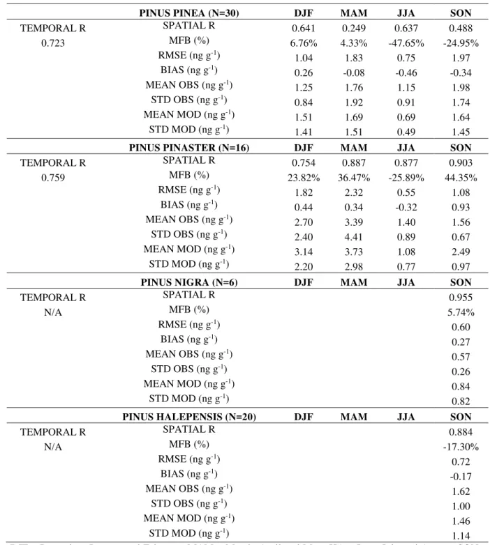
Table 1 – Seasonal evaluation of modelling results (over vegetal canopies) against pine 581
needle data according to the sampling periods of each pine species. 582
PINUS PINEA (N=30) DJF MAM JJA SON
TEMPORAL R SPATIAL R 0.641 0.249 0.637 0.488 0.723 MFB (%) 6.76% 4.33% -47.65% -24.95% RMSE (ng g-1) 1.04 1.83 0.75 1.97 BIAS (ng g-1) 0.26 -0.08 -0.46 -0.34 MEAN OBS (ng g-1) 1.25 1.76 1.15 1.98 STD OBS (ng g-1) 0.84 1.92 0.91 1.74 MEAN MOD (ng g-1) 1.51 1.69 0.69 1.64 STD MOD (ng g-1) 1.41 1.51 0.49 1.45
PINUS PINASTER (N=16) DJF MAM JJA SON
TEMPORAL R SPATIAL R 0.754 0.887 0.877 0.903 0.759 MFB (%) 23.82% 36.47% -25.89% 44.35% RMSE (ng g-1) 1.82 2.32 0.55 1.08 BIAS (ng g-1) 0.44 0.34 -0.32 0.93 MEAN OBS (ng g-1) 2.70 3.39 1.40 1.56 STD OBS (ng g-1) 2.40 4.41 0.89 0.67 MEAN MOD (ng g-1) 3.14 3.73 1.08 2.49 STD MOD (ng g-1) 2.20 2.98 0.77 0.97
PINUS NIGRA (N=6) DJF MAM JJA SON
TEMPORAL R SPATIAL R 0.955 N/A MFB (%) 5.74% RMSE (ng g-1) 0.60 BIAS (ng g-1) 0.27 MEAN OBS (ng g-1) 0.57 STD OBS (ng g-1) 0.26 MEAN MOD (ng g-1) 0.84 STD MOD (ng g-1) 0.82
PINUS HALEPENSIS (N=20) DJF MAM JJA SON
TEMPORAL R SPATIAL R 0.884 N/A MFB (%) -17.30% RMSE (ng g-1) 0.72 BIAS (ng g-1) -0.17 MEAN OBS (ng g-1) 1.62 STD OBS (ng g-1) 1.00 MEAN MOD (ng g-1) 1.46 STD MOD (ng g-1) 1.14
DJF – December, January and February; MAM – March, April and May; JJA – June, July and August; SON –
583
September, October and November; MFB - mean fractional bias; RMSE - root mean square error; OBS - pine
584
needle concentrations; MOD - modelled concentrations; STD – standard deviation; R – correlation coefficient; N
585
– number of sampling sites
586 587
Table 2 – Results from the comparison of BaP concentrations in air obtained by the chemistry 588
transport model simulations and those estimated from pine needle levels by St. Amand et al. 589
(2007, 2009a, 2009b), grouped by pine species. 590
PINUS PINEA (N=30) DJF MAM JJA SON
TEMPORAL R SPATIAL R 0.678 0.819 0.426 0.934 0.727 MFB (%) -43.26% -47.18% -28.46% -5.80% RMSE (pg m-3) 12.43 8.82 5.78 4.99 BIAS (pg m-3) -6.60 -5.27 -2.10 -0.66 MEAN ST. AMAND (pg m-3) 8.70 10.22 5.00 8.07 STD ST. AMAND (pg m-3) 5.88 10.11 3.97 7.59 MEAN CTM (pg m-3) 13.29 11.79 5.46 8.73 STD CTM (pg m-3) 13.22 11.57 5.08 8.17
PINUS PINASTER (N=16) DJF MAM JJA SON
TEMPORAL R SPATIAL R 0.627 0.838 0.929 0.486 0.703 MFB (%) 49.60% 25.66% 28.78% -3.73% RMSE (pg m-3) 21.60 14.19 4.01 13.08 BIAS (pg m-3) 11.20 6.25 1.17 -2.72 MEAN ST. AMAND (pg m-3) 28.43 23.27 8.84 8.41 STD ST. AMAND (pg m-3) 23.78 21.42 5.62 3.78 MEAN CTM (pg m-3) 15.28 16.83 7.64 11.12 STD CTM (pg m-3) 14.53 16.19 7.59 10.58
PINUS NIGRA (N=6) DJF MAM JJA SON
TEMPORAL R SPATIAL R 0.755 N/A MFB (%) -67.86% RMSE (pg m-3) 2.19 BIAS (pg m-3) -1.95 MEAN ST. AMAND (pg m-3) 1.91 STD ST. AMAND (pg m-3) 0.87 MEAN CTM (pg m-3) 3.85 STD CTM (pg m-3) 1.33
PNUS HALEPENSIS (N=20) DJF MAM JJA SON
TEMPORAL R SPATIAL R 0.381 N/A MFB (%) 8.94% RMSE (pg m-3) 2.69 BIAS (pg m-3) 0.88 MEAN ST. AMAND (pg m-3) 4.04 STD ST. AMAND (pg m-3) 2.49 MEAN CTM (pg m-3) 3.17 STD CTM (pg m-3) 0.98
DJF – December, January and February; MAM – March, April and May; JJA – June, July and August; SON –
591
September, October and November; MFB - mean fractional bias; RMSE - root mean square error; STD –
592
standard deviation; R – correlation coefficient; N – number of sampling sites
593 594
FIGURES
595 596
597
Figure 1 – (Top) Annual modelled deposition of BaP on vegetation (ng g-1) over the domain
598
covering the Iberian Peninsula. (Bottom) Seasonal contribution (%) to the annual total 599
concentration over vegetation: (from top-down and left-right): winter (DJF), spring (MAM), 600
602
603
Figure 2 – BaP mean annual climatology in air (pg m-3) over the Iberian Peninsula (mean
604
values for the period 2006-2010). 605
606 607
0,0 0,5 1,0 1,5 2,0 2,5 3,0 F M F M F M F M
P. pinea P. pinaster P. nigra P. halepensis
B a P ( n g g -1) 608
Figure 3 – Mean deposition levels (ng g-1) on pine needles for all samples, grouped by pine
609
species (F: field; M: CTM modelling). The black line on the bars represents the standard 610 deviation. 611 612 613 0 2 4 6 8 10 12 14 16 18 M S M S M S M S
P. pinea P. pinaster P. nigra P. halepensis
B a P ( p g m -3) 614
Figure 4 – Mean atmospheric concentrations (pg m-3) as estimated by CTM modelling (M)
615
and air-vegetation estimation (S) by St. Amand et al (2007, 2009a, 2009b). The black line on 616
the bars represents the standard deviation. 617