Article
Calculating the uncertainty associated to the forecast of species
dispersals: Stochastic Flow Connectivity
Alessandro Ferrarini
Department of Evolutionary and Functional Biology, University of Parma, Via G. Saragat 4, I-43100 Parma, Italy E-mail: [email protected], [email protected], [email protected]
Received 21 October 2015; Accepted 30 November 2015; Published online 1 March 2016
Abstract
To date, corridors for species dispersals have been thought as deterministic outputs emerging from some kind of model. Uncertainty about the individuation of biotic corridors has never been considered. Flow connectivity (FC) is a methodology first introduced in 2013 to forecast biotic flows over real landscapes, alternative to both circuit theory and least-cost modelling. Its name is due to the fact that it resembles in some way the motion characteristic of fluids over a surface. FC predicts species dispersal by minimizing at each time step the potential energy due to fictional gravity force over a frictional 3D landscape built upon the real landscape. In this work, FC is further developed to find a solution to the problem of calculating the uncertainty associated to the forecast of species dispersals. The output of this method is an “uncertainty polygon” (e.g., 5% or 10% uncertainty) around the predicted biotic flow. The importance of this new variant of FC is clear: when planning greenways for biodiversity, uncertainty about biotic flows prediction must be taken into account and the planned corridors must encompass the “uncertainty polygon” as well, otherwise they are at serious risk to underestimate the necessary space required by animal species to flow over landscape.
Keywords biotic flows; dynamical GIS; flow connectivity; gene flow; landscape connectivity; species dispersal; sensitivity analysis; uncertainty.
1Introduction
Flow connectivity (FC hereafter) is a methodology first introduced in 2013 (Ferrarini, 2013) to forecast biotic flows over real landscapes, alternative to circuit theory (McRae, 2006; McRae and Beier, 2007; McRae et al., 2008) and least-cost modelling (Dijkstra, 1959). Its name is due to the fact that it resembles in some way the motion characteristic of fluids over a surface. In fact, FC predicts species dispersal by minimizing at each time step the potential energy due to fictional gravity force over a frictional 3D landscape built upon the real landscape. FC considers connectivity to be a function of a continuous gradient of permeability values rather
Computational Ecology and Software ISSN 2220721X
URL: http://www.iaees.org/publications/journals/ces/onlineversion.asp RSS: http://www.iaees.org/publications/journals/ces/rss.xml
Email: [email protected] EditorinChief: WenJun Zhang
than attempting to distinguish discrete patches based on subjective thresholds of habitat area, quality, or ownership. A comparison with circuit theory and least-cost modelling are discussed in Ferrarini (2013) and Ferrarini (2014e).
At present FC presents many variants (Table 1), each devoted to a particular topic of species dispersals over landscape. In this paper, I introduce a new variant called Stochastic FC, aimed to calculate uncertainty associated to the individuation of biotic corridors of species dispersals. The output of this method is an “uncertainty polygon” (e.g., 5% or 10% uncertainty) around the predicted biotic flow. The importance of this new variant to FC is clear: when planning greenways for biodiversity, uncertainty about biotic flows prediction must be taken into account and the planned corridors must encompass the “uncertainty polygon” as well, otherwise they are at serious risk to underestimate the necessary space required by animal species to flow over landscape.
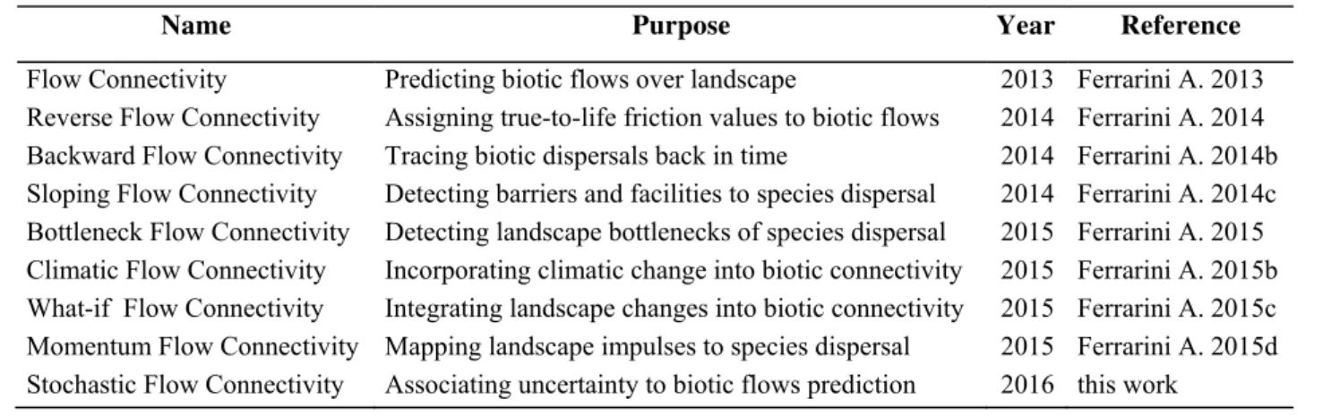
Table 1 Flow Connectivity and its developed variants, each with a particular purpose.
Name Purpose Year Reference
Flow Connectivity Predicting biotic flows over landscape 2013 Ferrarini A. 2013
Reverse Flow Connectivity Assigning true-to-life friction values to biotic flows 2014 Ferrarini A. 2014
Backward Flow Connectivity Tracing biotic dispersals back in time 2014 Ferrarini A. 2014b
Sloping Flow Connectivity Detecting barriers and facilities to species dispersal 2014 Ferrarini A. 2014c Bottleneck Flow Connectivity Detecting landscape bottlenecks of species dispersal 2015 Ferrarini A. 2015 Climatic Flow Connectivity Incorporating climatic change into biotic connectivity 2015 Ferrarini A. 2015b What-if Flow Connectivity Integrating landscape changes into biotic connectivity 2015 Ferrarini A. 2015c Momentum Flow Connectivity Mapping landscape impulses to species dispersal 2015 Ferrarini A. 2015d Stochastic Flow Connectivity Associating uncertainty to biotic flows prediction 2016 this work
2 Stochastic Flow Connectivity: Mathematical Formulation
Let
L x y z t
( , , , )
be a real 3D landscape at generic time t, whereL[1,..., ]n . In other words, L is a generic(categorical) landcover (or land-use) map with n classes. At time T0,
0
( , , , )
0L
L x y z t
(1)Let
( )
L
be the landscape friction (i.e. how much each land parcel is unfavorable) to the species under study.In other words,
( )
L
is a function that associates a friction value to each pixel of L. Landscape friction has 2components (structural and functional) and the overall friction should be equal to their product since they’re interactive:
( )
L
STR( ) *
L
FUNC( )
L
(2)At time T0,
(
L
)
Let
L x y
s( , , ( ))
L
be a landscape where, for each pixel, the z-value is equal to the friction for the speciesunder study. In other words, Ls is a 3D fictional landscape with the same coordinates and geographic
projection as L, but with pixel-by-pixel friction values in place of real z-values. Higher elevations represents areas with elevated friction to the species due to whatever reason (unsuitable landcover, human disturbance etc), while lower altitudes represent the opposite. At time T0,
0
( , , (
0))
s s
L
L x y
L
(4)
Let
S x y t
( , , )
be a binary landscape (of which Sxyt represents the value of the generic pixel at time t) withthe same coordinates and geographic projection as Ls and L, but with binary values at each pixel representing
species presence/absence at generic time t. At time T0,
0
( , , )
0S
S x y t
(5)FC simulates biotic flows over the frictional landscape Ls as follows (Ferrarini 2013)
( , , )
div
S x y t
S
S
S
S
t
x
y
(6)with initial conditions
S
0 at time T0. The symbol δ is a notation for a differential (i.e.
) or a difference (i.e. Δ) partial equation depending on the kind of landscape under study. For a high-resolution frictional landscape it represents a differential operator that simulates almost continuous movements over such landscape, conversely for a low resolution landscape it describes discrete movements both in space and time.As showed in Ferrarini (2013), the equation of resulting biotic flow can be solved as follows:
0
0
1 (
1
0)
(
0
1)
1
S
S
if
x
y
S
S
S
if
and
t
x
y
S
S
or
and
x
y
S
S
or
x
y
(7)FC assumes that the species dispersal ends at a stability point, if exists, where:
( , , )
0
S x y t
S
t
(8)True-to-life coefficients for
( )
L
can be calculated in flow connectivity as depicted in Ferrarini (2014), whereI defined P as the predicted path for the species over the fictional landscape Ls, and P* the real path followed
by the species (as detected by GPS data-loggers or in situ observations). The bias B between P and P* is hence calculated as
*
mod(
)
B
Pdx
P dx
(9)where the function mod indicates the module of the difference. Hence:
* *
* *
where >
where
>
Pdx
P dx
P P
B
P dx
Pdx
P P
(10)True-to-life coefficients for landscape friction can now be calculated by optimizing B, as follows:
set B to 0 (11)
or, at least,
minimize B (12)
In other words, FC assigns realistic resistance values to each land cover type by making null the bias B between the predicted dispersal and the detected one. To do this, it builds up the optimized fictional
landscape
L x y
s( , , ( ))
L
so that the predicted biotic flow P corresponds to the one (i.e. P*) detected in situ.The optimization of
( )
L
can be properly achieved using genetic algorithms (GAs; Holland, 1975). GAs arepowerful evolutionary models with wide potential applications in ecology and biology, such as optimization of protected areas (Parolo et al., 2009), optimal sampling (Ferrarini, 2012a; Ferrarini, 2012b), optimal detection of landscape units (Rossi et al., 2014) and networks control (Ferrarini, 2011; Ferrarini, 2013b; Ferrarini, 2013c; Ferrarini, 2013d; Ferrarini, 2013e; Ferrarini, 2014d).
Alternatively, a simpler solution used by FC to the assessment of realistic friction coefficients is the application of suitability modelling to the detected points of species presence over the landscape. In particular, MAXENT methodology (Phillips et al., 2006) is particularly well suited to determine suitability maps starting
from points of species presence. MAXENT computes the suitability scores
( )
L
for each portion of the landscape in the 0-100 range. Thus, friction coefficients can be properly calculated as complementary to 100 of suitability:( )
100
( )
L
L
(13)Although the achieved frictional coefficients should be considered reliable (as they’re based on in situ experiments), uncertainty about the achieved optimized coefficients can be simulated by FC as follows
(14)
where
~
i
(15)
or alternatively
(16)
In other words, represents a 5% (or 10%) uncertainty about φ(L) for each generic k-th landscape pixel.
If we stochastically vary n times (e.g. 10,000 times) φ(L) for each generic k-th landscape pixel, we can compute n predicted biotic flows around the predicted (deterministic) one. The minimum circumscribed polygon around such n paths hence represents the 5% (or 10%) uncertainty boundary due to our uncertainty about the landscape friction at each k-th landscape pixel.
3 An Applicative Example
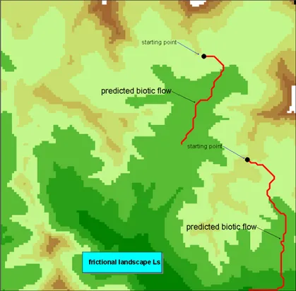
The Ceno valley is a 35,038 ha wide valley situated in the Province of Parma, Northern Italy. It has been mapped at 1:25,000 scale (Ferrarini, 2005; Ferrarini et al., 2010) using the CORINE Biotopes classification system. The landscape structure of the Ceno Valley has been widely analyzed (Ferrarini and Tomaselli, 2010; Ferrarini, 2011b; Ferrarini, 2012c; Ferrarini, 2012d). Several wolf populations have been recently observed in situ by life-watchers, environmental associations and local administrations. I have applied stochastic FC to a portion of the Ceno valley above 1000 m a.s.l. close to the municipality of Bardi (Fig. 1).
Fig. 1 The frictional landscape Lshas been built for wolf upon a portion (20 km * 20 km) of the Ceno valley (province of Parma,
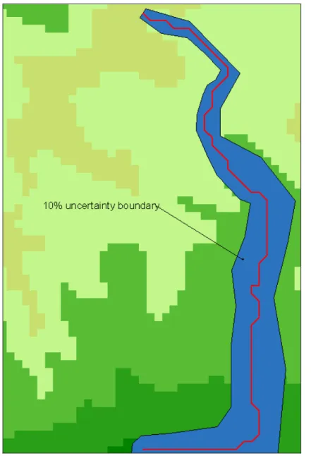
The area is a square of about 20 km * 20 km. Optimized friction valuesto wolf presence are borrowed from Ferrarini (2012e). Stochastic FC applied to the predicted dispersal routes of Fig 1 provides the results depicted in Fig. 2 and Fig 3. Red lines represent the predicted biotic flows, while blue polygons depict the 10% uncertainty polygons about the predicted dispersal routes. For each pixel of the frictional landscape, a 10% uncertainty has been simulated and 1000 random values in the 10% uncertainty interval have been simulated. This mean, for instance, that during simulations a pixel with a friction value equal to 5 can get any values in the range [4.5, 5.5]. This has been realized 1000 times for each pixel, and each time the resulting biotic flow has been recalculated. The resulting uncertainty polygons (in blue in Figs. 2 and 3) depict safety corridors that take into account not only the supposed ecological requirements of the study species while shifting over the landscape, but also the uncertainty of our knowledge about its requirements.
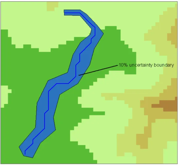
The minimum width around the predicted flows is 15.78 m in Fig. 2 and 16.78 m in Fig. 3 respectively, while the maximum width of the uncertainty boundary is 78.45 m in Fig. 2 and 82.87 m in Fig. 3.
Fig. 3 Application of stochastic Flow Connectivity to one of the two predicted dispersal routes of Fig. 1. For each pixel of the frictional landscape, a 10% uncertainty has been simulated using 1000 random values in a 10% uncertainty interval and each time the resulting biotic flow has been recalculated.
An important result emerges from previous simulations: all other things being equal, the uncertainty about how species dispersals happen is much higher when the surrounding frictional landscape is homogeneous, i.e. landscape friction varies slowly. In Figs. 2 and 3 it can be seen that at the beginning of the dispersal paths the landscape friction varies quickly and the uncertainty polygon is narrow. Instead, in the middle and ending parts of the paths, friction varies little and slowly and the uncertainty boundary becomes much larger. This suggests that Stochastic Flow Connectivity is particularly useful for hilly and mountain landscapes where the land cover is very homogeneous, and the uncertainty about biotic corridors increases.
In order to apply stochastic FC modelling to real landscapes, I wrote the ad hoc software Connectivity Lab (Ferrarini, 2013f).
4 Conclusions
In this work, Flow Connectivity has been extended to find a solution to the problem of calculating the uncertainty associated to the prediction of biotic flows. The output of this method is an “uncertainty polygon” (e.g., 5% or 10% uncertainty) around the predicted biotic flow.
Together with previous variants, stochastic Flow Connectivity represents a further contribution to the realistic forecast of biotic and gene flows over real landscapes with application to landscape genetics, landscape ecology and species conservation.
References
Dijkstra EW. 1959. A note on two problems in connexion with graphs. Numerische Mathematik, 1: 269-271 Ferrarini A. 2005. Analisi e valutazioni spazio-temporale mediante GIS e Telerilevamento del grado di
Pressione Antropica attuale e potenziale gravante sul mosaico degli habitat di alcune aree italiane. Ipotesi di pianificazione. Ph.D. Thesis, Università degli Studi di Parma, Parma, Italy
Ferrarini A, Bollini A, Sammut E. 2010. Digital Strategies and Solutions for the Remote Rural Areas Development. Acts of Annual MeCCSA Conference, London School of Economics, London, UK
Ferrarini A, Tomaselli M. 2010. A new approach to the analysis of adjacencies. Potentials for landscape insights. Ecological Modelling, 221: 1889-1896
Ferrarini A. 2011. Some thoughts on the controllability of network systems. Network Biology, 1(3-4): 186-188 Ferrarini A. 2011b. Network graphs unveil landscape structure and change. Network Biology, 1(2): 121-126 Ferrarini A. 2012a. Biodiversity optimal sampling: an algorithmic solution. Proceedings of the International
Academy of Ecology and Environmental Sciences, 2(1): 50-52
Ferrarini A. 2012b. Betterments to biodiversity optimal sampling. Proceedings of the International Academy of Ecology and Environmental Sciences, 2(4): 246-250
Ferrarini A. 2012c. Founding RGB Ecology: the Ecology of Synthesis. Proceedings of the International Academy of Ecology and Environmental Sciences, 2(2):84-89
Ferrarini A. 2012d. Landscape structural modeling. A multivariate cartographic exegesis. In: Ecological Modeling (Zhang WJ, ed). 325-334, Nova Science Publishers Inc., USA
Ferrarini A. 2012e. The ecological network of the province of Parma. Province of Parma, Parma, Italy, 124 pages (in Italian)
Ferrarini A. 2013. A criticism of connectivity in ecology and an alternative modelling approach: Flow connectivity. Environmental Skeptics and Critics, 2(4): 118-125
Ferrarini A. 2013b. Controlling ecological and biological networks via evolutionary modelling. Network Biology, 3(3): 97-105
Ferrarini A. 2013c. Computing the uncertainty associated with the control of ecological and biological systems. Computational Ecology and Software, 3(3): 74-80
Ferrarini A. 2013d. Exogenous control of biological and ecological systems through evolutionary modelling.
Proceedings of the International Academy of Ecology and Environmental Sciences, 3(3): 257-265
Ferrarini A. 2013e. Networks control: Introducing the degree of success and feasibility. Network Biology, 3(4): 127-132
Ferrarini A. 2013f. Connectivity-Lab 2.1: a software for applying connectivity-flow modelling. Manual, 104 pages (in Italian)
Ferrarini A. 2014b. Can we trace biotic dispersals back in time? Introducing backward flow connectivity. Environmental Skeptics and Critics, 3(2): 39-46
Ferrarini A. 2014c. Detecting barriers and facilities to species dispersal: introducing sloping flow connectivity. Proceedings of the International Academy of Ecology and Environmental Sciences, 4(3): 123-133
Ferrarini A. 2014d. Local and global control of ecological and biological networks. Network Biology, 4(1): 21-30
Ferrarini A. 2014e. Ecological connectivity: Flow connectivity vs. least cost modelling. Computational Ecology and Software, 4(4): 223-233
Ferrarini A. 2015. Where do they come from? Flow connectivity detects landscape bottlenecks. Environmental Skeptics and Critics, 4(1): 27-35
Ferrarini A. 2015b. Incorporating climatic change into ecological connectivity: Climatic Flow Connectivity. Computational Ecology and Software, 5(1): 63-68
Ferrarini A. 2015c. Integrating landscape changes into ecological connectivity: What-if flow connectivity. Proceedings of the International Academy of Ecology and Environmental Sciences, 5(2): 77-82
Ferrarini A. 2015d. Mapping landscape impulses to species dispersal: Momentum Flow Connectivity. Environmental Skeptics and Critics, 4(3): 81-88
Holland JH. 1975. Adaptation in Natural And Artificial Systems: An Introductory Analysis with Applications to Biology, Control and Artificial Intelligence. University of Michigan Press, Ann Arbor, USA
McRae BH. 2006. Isolation by resistance. Evolution, 60: 1551-1561
McRae BH, Beier P. 2007. Circuit theory predicts gene flow in plant and animal populations. Proceedings of the National Academy of Sciences of the USA, 104: 19885-19890
McRae BH, Dickson BG, Keitt TH, Shah VB. 2008. Using circuit theory to model connectivity in ecology and conservation. Ecology, 10: 2712-2724
Parolo G, Ferrarini A, Rossi G. 2009. Optimization of tourism impacts within protected areas by means of genetic algorithms. Ecological Modelling, 220: 1138-1147
Phillips SJ, Anderson RP, Schapire RE. 2006. Maximum entropy modelling of species geographic distributions. Ecological Modelling, 190: 231-259