2019
UNIVERSIDADE DE LISBOA FACULDADE DE CIÊNCIAS DEPARTAMENTO DE BIOLOGIA ANIMAL
Optimizing the reproductive development of the sea
cucumber Holothuria (Panningoturia) forskali Delle Chiaje, 1823 in
captivity: advances for the species’ aquaculture
João Trigo de Sousa
Mestrado em Ecologia Marinha
Dissertação orientada por Doutora Ana C. Brito Doutor Pedro M. Félix
ii
iii List of figures ... iv List of tables ... v Acknowledgements ... vi Resumo ... vii Abstract ... viii 1. Introduction ... 1
1.1.Sea cucumber exploitation ... 2
1.2. Sea cucumber aquaculture: State of the art ... 3
1.3. Sea cucumber nutritional potential ... 5
1.4. Biology of Holothuria forskali ... 6
2.Objectives ... 9
3. Materials and Methods ... 10
3.1. Capture and transport ... 10
3.2. Captivity conditions ... 11 3.3. Histological analysis ... 14 3.4. Lipid content... 16 3.5. Protein content ... 18 3.6. Statistical analysis ... 19 4.Results ... 19
4.1. Capture and transport ... 19
4.2. Captivity conditions ... 20
4.3. Histological analysis ... 25
4.4. Lipid content... 30
4.5. Protein Content ... 30
5.Discussion ... 31
5.1. Capture, transport and acclimation ... 31
5.2. Body mass and mortality rate ... 32
5.3. Gonadosomatic index ... 34 5.4. Histological analysis ... 34 5.5. Biochemical analysis ... 35 6.Conclusion ... 36 7.Future perspectives ... 36 References ... 38 Annexes ... 46 Contents
iv
List of figures
Fig 1.1.1 - Hypothetical variations in stock abundance under two different harvest strategies: pulse fishing and modest continuous fishing. Fishing periods are denoted by dashed curves; periods of fishing closures are denoted by solid curves. Under a ‘closure-pulse fishing-closure’ strategy, populations are reduced at a faster rate than under a modest continuous fishing strategy and risk falling below levels at which depensatory (Allee) effects occur. (a) The Allee threshold is low and stock abundance is not suppressed below it during the intensive pulse fishing and stocks recover thereafter. (b) The Allee threshold is slightly higher causing stock abundance after the second pulse fishing period to be below the level at which per
capita growth of the population is positive, and the population fails to recover thereafter (Adapted from
Purcell et al, 2013). ... 2
Fig 1.4.1 - Shape and colour of an individual of Holothuria forskali. (A) Dorsal side (bivium); (B) Ventral side (trivium). ... 6
Fig 1.4.2 - Geographic range of Holothuria forskali (IUCN, 2018) ... 7
Fig 1.4.3 - Shape and colour of female (left) and male (right) Holothuria forskali gonads. ... 8
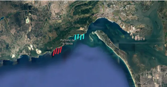
Fig 3.1.1. - Coastal area of Arrábida where sampling took place (delimited area). ... 10
Fig 3.2.1 - Example of the RAS used during the trial (A = sandy substrate, B = protein skimmer; C = mechanical filtration by the means of wool and sponge filters, D = Biological filtration by the means of plastic bio-balls, E = Water chiller). ... 12
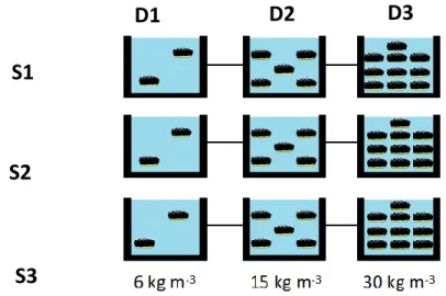
Fig 3.2.2 - Schematic representation of the trial settings for H. forskali along the different RAS (designated as S1, S2 and S3) and in accordance with their respective densities (designated as D1, D2 and D3). ... 12
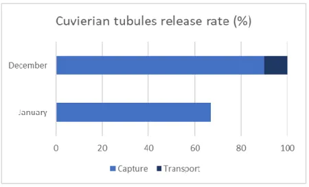
Fig 4.1.1 - Comparing Cuvierian tubules’ release rate of Holothuria forskali between capture and transport in December and January... 20
Fig 4.2.1 - Total evisceration and mortality rates of Holothuria forskali during the acclimation period between December and January. ... 20
Fig 4.2.2 - Mortality rate of Holothuria forskali according to the different densities in question at the end of the trial (D1 = 6 kg.m-3; D2 = 15 kg.m-3; D3 = 30 kg.m-3). ... 21
Fig 4.2.3 - Mean fresh weight (±SD) in individuals of Holothuria forskali in the beginning (January) and the end (May) of the trial (D1 = 6 kg.m-3; D2 = 15 kg.m-3; D3 = 30 kg.m-3). *Statistically significant differences between January (trial onset) and May (trial end). ... 22
Fig 4.2.4. - Mean gutted weight (±SD) in individuals in the beginning (January) and at the end (May) of the trial (t0 = Baseline group; D1 = 6 kg.m-3; D2 = 15 kg.m-3; D3 = 30 kg.m-3). *Statistically significant differences between January (trial onset) and each May group (trial end). ... 23
Fig 4.2.5. - Mean relative available mass (±SD) of individuals in the beginning (January) and at the end (May) of the trial (t0 = Baseline group; D1 = 6 kg.m-3; D2 = 15 kg.m-3; D3 = 30 kg.m-3)... 24
Fig 4.2.6 - Variation of mean gonadosomatic Index (±SD) in Holothuria forskali in the beginning (January) and at the end (May) of the trial (t0 = Baseline group; D1 = 6 kg.m-3; D2 = 15 kg.m-3; D3 = 30 kg.m-3; Wild = Wild individuals collected at the end of the trial). *Statistically significant differences between each group and wild individuals in May (trial end)... 25
Fig 4.3.1 - Sex Ratio of Holothuria forskali according to Stock Density. (F) Female; (M) Male; (U) Undetermined. (t0 = Baseline group; D1 = 6 kg.m-3; D2 = 15 kg.m-3; D3 = 30 kg.m-3). ... 26
Fig 4.3.2. - Microscopic characteristics of different gonadal stages in Holothuria forskali. (A) Growing stage on a female individual; (B) Growing stage on a male individual; (C) Mature stage on a female individual; (D) Mature stage on a male individual; (E) Post-Spawning stage on a female individual; (F) Post-Spawning stage on a male individual. (DO) Developing Oocyte; (GW) Gonadal wall; (L) Lumen; (MO) Mature oocyte; (RO) Relict oocyte; (Sc) Spermatocyte; (Sz) Spermatozoa. ... 27
Fig 4.3.3 - Relative frequency of each developmental stage recorded in the sampled male (M) and female (F) individuals according to their different stock densities (t0 = Baseline group; D1 = 6 kg.m-3; D2 = 15 kg.m-3; D3 = 30 kg.m-3)... 28 List of figures List of figures List of figures List of figures List of figures List of figures List of figures List of figures List of figures List of figures List of figures List of figures List of figures
v Fig 4.3.4 - Mean oocyte diameter registered in individuals according to their different stock densities (t0 =
Baseline group; D1 = 6 kg.m-3; D2 = 15 kg.m-3; D3 = 30 kg.m-3). ... 28
Fig 4.3.5 - Length and relative frequency of female oocytes in sampled Holothuria forskali (t0 = Baseline
group; D1 = 6 kgm-3; D2 = 15 kgm-3; D3 = 30 kgm-3) with moving average trendline (Red). ... 29
Fig 4.4.1 - Total Lipid content present in sampled muscle tissue of Holothuria forskali in the beginning (January) and at the end (May) the trial (t0 = Baseline group; D1 = 6 kgm-3; D2 = 15 kgm-3; D3 = 30 kgm-3;
Wild = Wild individuals collected at the end of the trial). ... 30 Fig 4.5.1 - Total protein content present in sampled muscle tissue of Holothuria forskali in the beginning (January) and at the end (May) of the trial (t0 = Baseline group; D1 = 6 kgm-3; D2 = 15 kgm-3; D3 = 30 kgm-3;
Wild = Wild individuals collected at the end of the trial). ... 31
List of tables List of Tables
Table 1.3.1: Nutritional composition (%) of fresh sea cucumbers (mean values ± SD). According to Ketharani & Sivashanthini (2016) ... 5 Table 4.2.1: Mean values (± SD) of the registered parameters across the different systems throughout the trial ... 21
vi
Acknowledgements
I would like to extend my gratitude first and foremost to my supervisors, Ana Brito and Pedro Félix, as well as my unsung supervisor Ana Pombo, without whom this work would have ended up in a completely different route. I thank them all for granting me this opportunity, for always being there for me whenever I stumbled on my path, for encouraging me to take new risks and continuously push my limits and most importantly, for their endless patience towards me.
I also thank the entire Newcumber team, in particular Tomás Simões and Francisco Azevedo e Silva, for their contagiously positive mood and ability to face adversity with an up-beat attitude, working with you guys is always a pleasure.
I would also like to thank my co-worker, Eliana Venâncio, for teaching me the ropes around the aquaculture lab, for always being by my side during the better times of the job, as well as the harsher, and for being a true friend both in and out of the lab. I honestly could not have asked for a better senior co-worker!
I can’t forget to thank my cousin Andreia Raposo, for always being available to give a helping hand, both in and out of the lab as well as prove that no matter where you go in this world you’re bound to run into family, no matter how distant.
I would like to thank the entire crew of MARE IPLeiria for welcoming me with open arms, there’s never a dull moment on the job.
I thank all my friends and family for all the support, jokes and curiosity shared on this journey of mine over an admittedly unusual topic, you guys turned good work better.
I thank my brother for believing I will one day be the most successful man in the family and this is but the first step to achieve that goal.
Lastly, I’d like to thank my mom and dad, for never doubting me on my path taken away from the family business, even when I came close to doubting myself. For all the support and all the encouragement, I can’t thank you both enough.
vii
Resumo
A elevada procura por pepinos-do-mar nos mercados internacionais, principalmente na Ásia, deixou um profundo impacto no stock natural de muitas espécies. Considerado um recurso alimentar altamente nutritivo, bem como um suplemento medicinal muito eficaz, os pepinos-do-mar do Indo-Pacífico foram explorados até a um ponto crítico, o que por sua vez levou a um alto investimento em aquacultura de modo a mitigar os efeitos negativos das pescas sobre as diversas espécies existentes e suprimir a escassez na oferta. Apesar dos diversos e consideráveis avanços neste sector, ainda existem poucos estudos focados inteiramente na gestão de reprodutores em cativeiro.
Este estudo teve como objetivo determinar o efeito de densidade em reprodutores para a produção de Holothuria (Panningoturia) forskali Delle Chiaje, 1823 em cativeiro, uma espécie comum no Mar Mediterrâneo e nordeste Atlântico, com potencial valor comercial. Para isso, foram consideradas três densidades diferentes, uma baixa de 6 kg.m-3, uma
média de 15 kg.m-3 e uma elevada de 30 kg.m-3.
O ensaio foi realizado ao longo de um período de cinco meses, sobre os quais os parâmetros de qualidade da água foram medidos diariamente, a fim de garantir uma qualidade estável da mesma. Uma vez terminado o ensaio, foi avaliado o efeito das densidades escolhidas no desenvolvimento dos indivíduos, nomeadamente quanto ao índice gonadossomático e conteúdo nutricional, bem como as taxas de evisceração e mortalidade.
O estudo efetuado sugere que a maior densidade, de 30 kg.m-3, é a que apresenta
melhores resultados para o acondicionamento de H. forskali em cativeiro por curtos períodos de tempo, embora testes adicionais sejam recomendados para determinar os efeitos por períodos mais longos.
Palavras chave: Equinoderme, reprodutores, densidade de stock, histologia, valor nutricional.
viii
Abstract
The high demand of sea cucumbers in international markets, mostly based in Asia, has left a deep impact on the natural stock of many different species. Considered a highly nutritious food resource as well as a very effective and ancient medicinal supplement, sea cucumbers across the Indo-Pacific have been exploited to a critical degree, which in turn led to a high investment in aquaculture in order to mitigate the negative impacts that fishing has had over the different species of sea cucumbers, as well as satisfy their continuous demand. Despite the much considerable advancements in this sector, few studies have yet to solely focus on the impact and management of broodstock in captivity.
This study aimed to determine the effects of stock density in rearing broodstock of
Holothuria (Panningoturia) forskali Delle Chiaje, 1823 in captivity, a common species in
the Mediterranean Sea and eastern Atlantic with a potential commercial value. To do so, three different densities were taken into consideration, a lower one of 6 kg.m-3, a medium
one of 15 kg.m-3 and a high one of 30 kg.m-3.
The trial took place over a period of five months, over which water quality parameters were measured daily in order to ensure a good water quality. At the end of the trial, the effects of stock density on the individuals’ condition were assessed, namely regarding their gonadosomatic index, nutritional content as well as evisceration and mortality rates.
Results obtained in this study point towards the highest density of 30 kg.m-3 being the
most beneficial for rearing H. forskali in captivity for short periods of time, although further testing is recommended to determine the effects for longer periods of time.
1
1. Introduction
The need to find and secure resources to sustain nutritional needs has been, and will always be, one of humanity’s paramount priorities. One such resource, rich in protein and commonly overlooked in the West, is the sea cucumber (Anderson, 2011).
Sea cucumbers are Echinoderms of the class Holothuroidea, in the Phylum Echinodermata, with high economic interest. All over the world, sea cucumber capturing techniques are extremely diverse both in methods and target-species. They vary from harvest by hand in shallow waters all the way to large-scale industrial fishing using diving and trawling (Kinch, 2008; Prescott, 2013).
Sea cucumbers are often traded as a dried product, known as Bêche-de-mer in french. They have been in high demand in China since ancient times (Fabinyi, 2011). Considered to be a delicacy and alleged to have favourable medicinal and strengthening effects, it holds strong ties to tradition, in particular festive occasions in south-eastern Asian countries or countries with deeply rooted Chinese communities (Chen, 2003). In China it is mostly consumed in a re-hydrated form while in Japan the intestine, gonad and longitudinal muscle are processed into exclusive gourmet products consisting mostly of stews and broths (FAO, 1988). Depending on the processing technique, rehydrated sea cucumbers can expand up to 6 or 7 times their dehydrated size (Chen & bean, 2012).
In recent years, however, securing enough resources to satisfy an ever-increasing human population has proven to be a challenging task, often leading to the over-exploration of available resources. The biggest impact occurs on natural fishing stocks, including sea cucumbers (Pauly et al., 2002), made worse by the inherent value of such a gourmet product. Many species of sea cucumbers are threatened mostly due to their high economic value, such as Apostichopus japonicus which can go for over US$3583 per dried kg
(Akamine, 2003; Conan et al, 2014; Purcell et al, 2014; Purcell et al, 2018).
The pressure from the high demand imposed on this group is such that their natural stock is dwindling, especially in certain regions of south-east Asia, mainly China, where the natural stock of certain species has been low for quite some time (Anderson, 2011). This steep decrease in abundance of wild sea cucumbers, along with the rising interest in consumption from the general public has led to high stakes arms race to grow and produce sea cucumbers in captivity in order to sustainably secure nutritional resources (Conand, 2004; FAO, 2012) as well as to secure a place in the competitive market of sea
2
cucumbers, allowing for a mitigation of the impact it has had on the many commercially viable species’ natural habitat (Auster, 1996; Friedman et al, 2011).
1.1. Sea cucumber exploitation
Due to their low motility, sea cucumbers are extremely susceptible to over-fishing, with high production cycles being closely followed by abrupt dips in population numbers, also known as pulse fishing, representing most of these captures (Zamora et al., 2016; Kinch et
al., 2008). Some authors however still advocate for a continuous fishing at a modest rate
(Purcell et al, 2011) as illustrated in fig. 1.1.1.
Fig 1.1.1 - Hypothetical variations in stock abundance under two different harvest strategies: pulse fishing and modest continuous fishing. Fishing periods are denoted by dashed curves; periods of fishing closures are denoted by solid curves. Under a ‘closure-pulse fishing-closure’ strategy, populations are reduced at a faster rate than under a modest continuous fishing strategy and risk falling below levels at which depensatory (Allee) effects occur. (a) The Allee threshold is low and stock abundance is not suppressed below it during the intensive pulse fishing and stocks recover thereafter. (b) The Allee threshold is slightly higher causing stock abundance after the second pulse fishing period to be below the level at which per capita growth of the population is positive, and the population fails to recover thereafter (Adapted from Purcell et al, 2011).
3
Resorting to reckless pulse fishing as demonstrated in the previous figure has led to recorded cases of stock decimation within 2-4 years in Egypt (Lawrence et al, 2004; Hasan 2005), Oman (Al-Rashdi and Claereboudt, 2010) and Tonga (Purcell et al, 2011). Unfortunately, despite the clear risks of stock decimation, the commercial demand for sea cucumbers has only gotten higher (Zamora et al, 2016), a demand that continuous fishing at a modest rate cannot possibly satisfy, leading to aquaculture development and improvement.
1.2. Sea cucumber aquaculture: State of the art
With fisheries being increasingly regulated in order to minimise the depletion of natural stocks, aquaculture has become a profitable industry and a helpful tool regarding the conservation of species (Purcell et al, 2011). Their goal is mostly focused on rearing individuals in order to supply the increasing demand from the food market, although some effort has been spared towards stock repopulation, with provisions having already been put in place regarding the breeding of juveniles aimed towards regions with a clear depletion in native species (Bell et al., 2008). In recent years, Aquaculture production has already exceeded its fisheries counterpart in global sea cucumber production (Fig 1.2.1.).
Fig 1.2.1 - Global wild captures and aquaculture production of sea cucumbers over time; in metric tonnes (t), (Adapted from Purcell et al, 2011).
4
Dating as far back as 1930, holothurian aquaculture has grown to unbelievable proportions, with the aquaculture production market value in China being estimated to exceed US$ 5 billion (Zhang et al, 2015), despite most of its techniques remaining generally unchanged at their core (Zamora et al, 2016). With its roots in Japan and mainland China, it has since expanded to India, Indonesia, the Maldives, Solomon Islands, Australia and certain regions of the western world (Battaglene, 1999). However, it still hasn’t managed to satisfy the ever-increasing demand from the general public (Anderson, 2011).
Regarding the aquaculture techniques, broodstock is preferably collected from the wild considering the genetic implications sprung from the repeated use of the same spawners, particularly if the main goal is stock repopulation. The collected sea cucumbers could be induced to spawn immediately or kept in land-based tanks to undergo conditioning towards captivity (Yanagisawa, 1998). Rapid and/or steep changes in water parameters, such as temperature, salinity and pH should be avoided while in captivity. During capture, sea cucumbers must be handled with extreme care. It is advisable to refrain from griping them too tightly or detaching them from substrate in an aggressive manner in order to avoid unwanted stress. Likewise, the same precautions regarding changes in water parameters must be taken into account with the added step of avoiding steep variations in the pressure at which the sea cucumbers are subjected to, so as to avoid unwanted early spawning, evisceration or even death (Ito, 1995; Yanagisawa, 1998).
While in captivity, broodstock are recorded to have been fed a variety of products, from dried brown algae in Japan, to soybean powder, rice bran, chicken manure, ground up algae and even prawn head waste in both India and Indonesia (James, 1996).
With sea cucumbers being considered a highly nutritional food resource, it is important to establish the most efficient diet in order to maximize somatic and/or gonadal growth, as well as enhance the nutritional potential of the many different species of sea cucumbers.
5
1.3. Sea cucumber nutritional potential
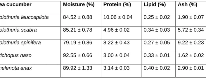
From a nutritional standpoint, sea cucumbers have been categorized as a delicacy with high nutritional value (Table 1.3.1.), with protein values as high as nearly 70% when dried (Chen, 2003). Having been consumed since the Ming Dynasty (1368-1644 AD) not only as a food source, but mainly as a tonic and traditional medicine with similar properties to Ginseng, hence its Chinese name, haishen, being roughly translated to Ginseng of the sea (Fabinyi, 2011). Historically used to treat fatigue, impotence, constipation, frailty resulting from old age and urinary incontinence (Huizeng, 2001), recent studies have more accurately determined the sea cucumbers health benefits resulted from their high content of polyunsaturated fatty acids (PUFA), particularly eicosapentaenoic acid (EPA) and docosahexaenoic acid (DHA) (Aydn et al, 2011).
Table 1.3.1: Nutritional composition (%) of fresh sea cucumbers (mean values ± SD). According to Ketharani & Sivashanthini (2016)
Sea cucumber Moisture (%) Protein (%) Lipid (%) Ash (%)
Holothuria leucospilota 84.52 ± 0.88 10.06 ± 0.04 0.25 ± 0.02 1.90 ± 0.07
Holothuria scabra 85.21 ± 0.78 4.96 ± 0.02 0.34 ± 0.03 5.72 ± 0.34
Holothuria spinifera 79.19 ± 0.86 8.22 ± 0.43 0.27 ± 0.05 9.22 ± 0.23
Stichopus naso 92.55 ± 0.66 3.00 ± 0.04 0.33 ± 0.01 1.62 ± 0.02
Thelenota anax 89.92 ± 1.33 3.14 ± 0.03 0.40 ± 0.02 2.90 ± 0.01
Aside from the rich protein content, some species of sea cucumbers produce toxins that have medicinal value, while others produce certain compounds that when isolated exhibit anti-microbial, anti-inflammatory, anti-oxidant (Ketharani & Sivashanthini, 2016; Santos et
al, 2015a; Santos et al, 2015b), anti-coagulant and immuno modulatory activities due to
the presence of compounds such as sulponamides and diketones (Aminin et al., 2001).
With the nutritional benefits in mind and its long history as a medicinal supplement (Chen, 2003; Gao et al, 2011; Zamora et al, 2016; Zhang et al, 2015) it’s easier to understand the value of the many different species of sea cucumbers.
6
Of these different species there is one highly abundant in the western world, just off the coast of Portugal, Holothuria forskali (Delle Chiaje, 1823), a potential resource that is yet to be fully explored.
1.4. Biology of Holothuria forskali
Holothuria (Panningoturia) forskali Delle Chiaje, 1823 is a considerably abundant species whose maximum-recorded fresh weight exceeds 200 g (Tuwo, 1992). Individuals from this species are characterized by having a dark tegument marked by small white spots that are visible under water, a yellow trivium and the presence of cuvierian tubules. Some specimens are less coloured, either dark brown or different shades of yellow (Fig 1.4.1). The distribution of the species is Atlanto-Mediterranean extending from Scandinavia and the British Isles to the Canary Islands and Morocco and along the northern Mediterranean coast (Koehler, 1927; Perez-Ruzafa & Lopez-Ibor, 1988), as illustrated by the figure 1.4.2. It is generally considered a littoral species commonly occurring in shallow waters (0-50 m of depth) on rocky reefs, especially on vertical surfaces (Southward & Campbell, 2006), therefore being characteristic of rocky bottoms although some exceptions have been found in sea-grass beds (Cherbonnier, 1958).
Fig 1.4.1 - Shape and colour of an individual of Holothuria forskali. (A) Dorsal side (bivium); (B) Ventral side (trivium).
7 Fig 1.4.2 - Geographic range of Holothuria forskali (IUCN, 2018)
As a defence mechanism and response to stress this species abruptly contracts their muscles in order to expel a thin and very adhesive organ called the Cuvierian tubules through its anus after a tear in the cloaca. This organ consists of several dozens, or even hundreds, of tubules whose proximal ends attach to the basal part of the left respiratory tree and whose distal, blind ends float freely in the coelomic cavity (Vandenspiegel, 2000). Sometimes the muscle contraction is so intense they end up expelling the rest of their internal organs in what is known as evisceration, however, under the appropriate conditions eviscerated individuals may be able to grow back their lost organs (Dimock, 1997). Sea cucumbers also possess a ventral mouth surrounded by a crown of 20 sensory tentacles that are used to evaluate the organically richest areas of sediment as well as for feeding (Bouland et al, 1982).
Regarding their reproductive system, although animals from this species do not present sexual dimorphism, they are in fact dioic, with females usually presenting larger gonads, known as ovaries (Tuwo, 1992). The ovaries are more vividly coloured, usually deep red, as opposed to their male counterpart (the testis), which are paler and slimmer, with a colouration closely resembling shades of yellow (Fig 1.4.3).
Fertilization of the eggs is done externally, requiring a significant density of individuals in order to maximize efficiency (Rakaj et al, 2017).
8 Fig 1.4.3 - Shape and colour of female (left) and male (right) Holothuria forskali gonads.
Although not yet compiled under FAO’s “Commercially important sea cucumbers of the world” (Purcell et al, 2012), Holothuria forskali is a commercially viable species already in the trade market (Alibaba, 2019), with potential for aquaculture production.
The rising surge in demand for sea cucumbers, including individuals from the species
Holothuria forskali, has been accompanied by a parallel increase in the development and
optimization of different techniques regarding broodstock maintenance in captivity. However, a key factor has been overlooked. While most studies aim towards optimizing diets (Yanagiswawa, 1998), hatchery techniques (Rakaj et al, 2017) or broodstock management (Battaglene, 1999), few studies focused on the effects different stock densities might have on the rearing of broodstocks. The most stand out case regarding this subject was centred on another species with high commercial value, Apostichopus
japonicus, and their optimal stock density in pond culture (Qin et al, 2009).
With most aquaculture studies focusing on species of fish with commercial interest, it is already established that higher densities will lead to negative consequences, such as higher mortality rates, lower growth rates and, from a commercial perspective, lower quality products (Ntanzi, 2014; Siracov, 2008). This study, in turn, focuses on the effects of stock density on the survival rate and overall quality of Holothuria forskali in Recirculating aquaculture systems (RAS).
9
2. Objectives
With few studies regarding the management of broodstock density in captivity, this study aimed to evaluate the effects that different stock densities may have in Holothuria forskali reared in captivity, including:
i) Their effect on evisceration and mortality rate, in order to determine the safest density for rearing in captivity;
ii) Their effect on body mass and gonadal development, in order to determine the density most suited towards broodstock rearing;
iii) Their effect on the amount of sea cucumber’s body mass available for human consumption (including gonads, muscle bands and body wall), in order to determine the most commercially viable density for stock rearing in captivity; iv) Their effect on protein and lipid content of muscle bands, in order to determine the
most suitable density for stock rearing in captivity aimed for human consumption.
To do so, this study sought to compare the effects of different stock densities based on previous studies, in particular, a low density (D1) of 6 kg.m-3, a medium (D2) of 15 kg.m-3
and a high (D3) of 30 kg.m-3. These three densities will help test the limits of broodstock
densities regarding aquaculture production, a step forward towards optimizing broodstock rearing conditions in captivity. This study also took into account the effects of stock density during transport and acclimation by comparing the results obtained from two capture campaigns in order to determine the least harmful density for the transport of live specimens.
10
3. Materials and Methods
3.1. Capture and transport
The sampled individuals (n=70) were captured in the coastal area of Arrábida (Fig 3.1.1) during two scuba diving campaigns that took place in December (n=40) and in January (n=30). All individuals were carefully collected by hand and placed in 46 L containers for transport, filled with seawater and with constant aeration. No additional sediment was added in order to minimize possible damage to the tegument (Santos, 2017). In December, specimens were stocked for transport at around 16 to 20 individuals per container (average 56.35 kg.m-3) while in January they were stocked at 12 individuals per container
(average 37.57 kg.m-3). At both occasions, all animals were conveyed to the Aquaculture
Lab of MARE-IPLeiria over a maximum period of 3 hours, with monitoring of any eventual lesion, evisceration and/or mortality.
11
3.2. Captivity conditions
Once the specimens arrived at the facilities, they were randomly assigned to a total of six tanks with 50 L capacity (38.5 x 34 x 38 cm), 3 for each sampling campaign in order to undergo a one-week minimum period of acclimation. This was done with the purpose of getting the captured sea cucumbers accustomed to the captivity conditions and subsequently assuring the individuals were under no stress from the sudden change in environment before the trial regarding the effects of stock density in captivity could begin. Due to the difference in number of captured individuals in the two campaigns, sea cucumbers collected in December were stocked for acclimation at an average density of 38.40 kg.m-3 while the ones collected in January were stocked at 28.80 kg.m-3. During the
placement of the animals into the tanks, transfer of debris and/or eviscerated material present in the transport containers was avoided.
When the acclimation period was over, all specimens were weighted individually in an analytical scale (ADAM PGL Precision Balance NDPGL4001, EUA) with a precision of 0.01 g. Ten individuals were selected randomly to determine their fresh and gutted weights, as well as their gonad weight, thus establishing a baseline comparison group comprised of both males and females, labelled as t0. After having their fresh, gutted and
gonad weights determined, individuals from t0 were then preserved at -20° C until the
biochemical analyses at the end of the trial.
With a mean fresh weight (± SD) of 144.35 ± 31.96 g, 51 Holothuria forskali were equitably distributed, according to a One-way ANOVA [F(8, 42) = 0.166; p = 0.994], into
tanks with a 50 L capacity, a bottom area of approximately 0.129 m2 and a surface (usable)
area of approximately 0.667 m2 (38.5 x 34 x 38 cm). These tanks were integrated in a
recirculation aquaculture system (RAS), with mechanical and biological filtration, continuous aeration, an air-cooled water chiller Frimar F200 (Fernando Ribeiro, Ltd., Barcarena, Portugal) and sandy substrate (Fig 3.2.1), according to the desired densities of:
i) 6 kg.m-3, designated as D1 (Chen, 2003; Xia 2017; Yang, 2005);
ii) 15 kg.m-3, designated as D2 (Chen & Chang, 2015);
12
All of the previously established densities were pulled from studies focused on species other than H. forskali and with different purposes, however they contributed towards the selection of a realistic starting point for the trial. Each of the selected densities had three replicates (designated as S1, S2 and S3) as depicted in figure 3.2.2. Individuals distributed by the experimental tanks at the onset of the trial presented no statistically significant differences with individuals from the baseline group (t0) in regards to their mean
fresh weight according to a One-Way ANOVA [F(3, 57) = 2.256; p = 0.092]. The statistical
similarity within stocked groups and between these and the baseline validated a common starting point that enabled comparisons between groups at the end of the trial.
Fig 3.2.1 - Example of the RAS used during the trial (A = sandy substrate, B = protein skimmer; C = mechanical filtration by the means of wool and sponge filters, D = Biological filtration by the means of plastic bio-balls, E = Water chiller).
Fig 3.2.2 - Schematic representation of the trial settings for H. forskali along the different RAS (designated as S1, S2 and S3) and in accordance with their respective densities (designated as D1, D2 and D3).
D1
D2
D3
S1
S2
S3
A
B
C
D
E
13
The trial lasted for a period of five months, with an established photoperiod of 12h light and 12h dark, over which the selected 51 H. forskali were fed three times a week a mixture of frozen microalgae composed of Tetraselmis sp. and Phaeodactylum tricornutum, two species of microalgae suitable for feeding individuals of this species (Santos, 2017).
Observations of the specimens occurred daily to record any occurrence of physiological alterations, evisceration and/or mortality. Water quality maintenance routines took place daily to ensure the well-being of the specimens, namely through water changes and removal of excreted products through siphoning, therefore reducing the probability of bacterial contamination and preventing significant changes to the water quality. To guarantee the control over abiotic conditions, water parameters were monitored through daily measurements of temperature (°C) and dissolved oxygen (mg.L-1) using a
multiparametric sonde (YSI-Pro Plus, USA), pH through a pH meter (SympHony SP70P, USA), ammonia, nitrates and nitrites (NH3, NH4+ and NO2- in mg.L-1) with colour tests (API,
U.S.A.), as well as salinity, measured with a refractometer (Seawater Refractometer #I96822, Romania).
At the end of the trial all surviving specimens were weighted, dissected and had their gonads collected. This task enabled the determination of their fresh and gutted weight after 5 months in captivity. By dividing the gutted weight over the fresh weight of each individual it was then possible to determine their relative available mass, which alongside the gonadosomatic index, can narrow down how much of a sea cucumber is available for human consumption and how much remains unconsumed (e.g. respiratory trees or stomach content like sand and debris). This mean relative available mass can help determine, from an economic standpoint, how much profit a sea cucumber stands to generate depending on the processing technique (Chen & Bean, 2012).
The gonad weight was also determined, which could then be used to calculate the sea cucumbers’ gonadosomatic index (GI) according to the following mathematical equation (Benítez-Villalobos et al., 2013):
14
Where,
Gw = Gonad weight (g);
Tw = Total gutted weight (g).
After being weighted, gonads were fixed in a buffered formaldehyde solution (4%) for a maximum of 48 hours before being preserved in alcohol (70%) for further histological analysis. Muscle tissue was also collected and preserved at -20 °C for further biochemical analysis (protein and lipid content).
At the end of the trial, complementary data (such as GI, lipid and protein content) were acquired from individuals captured in the month of May from the coast of Arrábida in order to determine the state of wild H. forskali. These parameters were registered in order to determine, by comparison, any physiological differences attained from rearing in captivity (i.e. ascertain any added value from controlled conditions in favour of gonad development and nutritional content).
3.3. Histological analysis
The extracted gonads that had been fixed were dehydrated in a tissue processor (Leica
TP1020, Germany)with sequential submersions in graded ethanol (80%, 96% and 99%),
followed by xylene for clarification and finally, impregnation with paraffin wax at 60º C, after which they were fixed in blocks of paraffin (Leica® EG 1120 Paraffin Dispenser with integrated Hot Plate, Leica Microsystems GmbH, Wetzlar, Germany), using Tissue-Tek stainless-steel base molds (Sakura Finetek Europe BV, Netherlands)and left to cool and solidify in a Kunz Instruments CP-4 Cooling Plate (Kunz Instruments, Denmark). Each block was then cut in a microtome (Sakura Accu - cut SRM 200, Japan), each cut having a thickness between 5 and 8 µm, and later fixed to a microscope slide for further coloration with Hematoxilin-Eosin and observation under an optic microscope (Leica DM 2000 LED, Germany). Each observed gonad cut was also photographed (Leica MC170 HD, Germany)
GI =
Gw
X 100
15
and had the diameter of the oocytes measured using the LAS software distance line tool, performed at 20X magnification (Software LAS V4.4, Germany). In each histological preparation were registered the diameter of 30 oocytes per female.
The analysed oocytes and spermatocytes were divided into five categories, based on the works of Despalatovic (2004), Kazanidis (2014) and Tuwu (1992), in accordance with their developmental stage as explained below:
Stage I - Recovery stage, where the female oogonia are embedded in the germinal layer. Small developing oocytes are arranged in a single layer. The gonad wall is thick and three basic layers are easily distinguished.
The males also present a thickening of the outer and inner epithelium of the gonad wall. Spermatogonia appear on the germinal layer, which may have numerous folds that increase the surface area for spermatogenesis.
Stage II - Growing stage, where the females have their germinal layer lined with oocytes at various stages of development. As vitellogenesis intensifies, fully-grown oocytes with large nuclei begin to take up a central position in the lumen of the tubules. Small follicular cells surround the oocytes. The gonad wall is still thick but in the advanced stages of growth it becomes narrower.
In the males this stage is characterized by very active spermatogenesis. Columns of spermatocytes extend towards the lumen and spermatozoa start to fill the lumen. As the growing proceeds, the folds of the germinal epithelium straighten out. The gonad wall is thinner and the follicles increase in size.
Stage III - Mature Stage, where the gonad wall is thin. In females, fully-grown mature oocytes that have reached their maximum size are densely packed in the lumen of tubules. In the germinal layer previtellogenic oocytes could be present and continuing their development.
The males present densely packed spermatozoa in the lumen of the tubules, which characterize mature testes. Spermatocyte columns are present in the germinal layer and spermatogenesis proceeds.
Stage IV - Spawning stage, where the females still present a thin gonad wall. There is a noticeable decrease in the abundance of oocytes inside the tubules. Empty spaces are observed in the lumen due to gamete release. The number of oocytes and the size of
16
empty spaces in the lumen depend on the stage of spawning. Few developing oocytes may remain in the germinal epithelium.
The males present spermatozoa less densely packed. Empty spaces are present in the lumen due to gamete release. In the early period of the spawning, a spermatogenic layer is present. There is an empty space between the spermatogenic layer and the mass of gametes in the central part of the lumen. The gonad wall is still very thin.
Stage V - Post-Spawning stage, where in females, the gonad wall is thick again and large amounts of connective tissue are present. Genital haemal sinus is present too. Unspawned relict oocytes are present in the lumen and start to show signs of degradation due to phagocytic activity.
Males In the post-spawning stage still present a very thick gonad wall and are characterized by the presence of large amounts of connective tissue. The genital haemal sinus starts to expand. Unspawned spermatozoa are present in the lumen. Phagocytosis is observed.
3.4. Lipid contents
In order to determine the total lipid contents of sea cucumber’s muscle bands, 3 random individuals from each stock density, as well as 3 preserved individuals from the t0 group,
were randomly selected at the end of the trial to have their muscle bands homogenized using an electric homogenizer (IKA T 18 D, Germany). To these 12 random individuals were added another 3 random sea cucumbers collected from the coastal area of Arrábida at the same time the trial had ended to assess any possible differences between wild individuals and individuals in captivity. After the initial preparation, the lipid content was determined by the Folch method (Folch et al. 1957). The selected individuals had 0.5 g of their fresh muscle bands extracted, homogenized and placed in a falcon tube alongside
2.5 mL of Folch reagent (CHCl3:MeOH 2.1) and mixed using a Pellet mixer (VWR Pellet
mixer, China) for 1 minute. The polytron head was rinsed with another 2.5 mL of Folch solution and vortexed for 5 minutes before being added 0.6 mL of NaCl 0.8% solution and vortexed again for another 2 minutes. After homogenization the mixture was centrifuged at 6000 rpm for 10 minutes at 4 °C using an automatic Centrifuge (Heidolph Laborota 4000, Germany) which resulted in two distinct phases, a top phase with the remainder of the
17
organic tissue and a lower phase containing the extracted lipids diluted in chloroform. The lower phase was meticulously collected with a 1 mL automatic pipette (Kartell SpA Pluripet PL-II 100 - 1000 μL, Italy), filtered through a sodium sulphate anhydrous column (Pasteur pipette with cotton on the bottom) and collected in an evaporator flask with known weight.
If there were any residuals of the lower phase, unable to be extracted due to its small volume, they would then be extracted by adding another 1 mL of CHCl3 to the mixture,
centrifuged at the same conditions and extracting the new lower phase in the same manner.
Finally, the solvent was evaporated under lower pressure using a rotary evaporator (Heidolph, Laborota 4000, Germany) and the lipid content was determined gravimetrically using an analytical scale (Sartorius Lab Instruments Gmb ENTRI224I - 1S, Germany) with a precision of 0.0001 g. The remaining additional weight to the evaporator flask would then translate to the total amount of lipids in the extracted sample according and the following formula:
Where,
Fw = Final weight of the evaporator flask (g)
Iw = Initial weight of the empty evaporator flask (g)
m = Sample mass (g)
Lipids (%) =
(Fw-Iw)
X 100
m
18
3.5. Protein contents
The protein contents were determined by way of the Kjeldahl method (Campbell, 1937). To do so, 0.5 g of homogenized muscle tissue, from each of the same individuals as the Lipid analysis, was placed in a digestive tube alongside 2 catalysing pills as well as 25 mL of sulfuric acid and identified accordingly. Once identified, the samples were placed in a digester (FOSS 2006 Digestor Unit DS6, Sweden) with the temperature set for 220 °C. In each digestion there was another tube with no samples to function as the blank solution.
After 30 minutes the temperature was raised to 400 °C where it stayed that way for another 90 minutes, after which the digester was turned off and the samples were left to cool for another 60 minutes. Digestion was considered finished once a clear liquid was obtained inside the tubes.
Once properly digested the tubes were distilled using a Distillation unit (FOSS 2100 Distillation Unit, Sweden). After being properly distilled, the resulting solutions from each sample, as well as the blanks, were then spiked with a solution of HCl at 0.1 M. With the volume spent to determine the solution’s turning point, the total protein content of the samples could be determined according to the following equation:
Where,
Vs = Volume of solution used to spike the sample (mL)
Vb = Volume of solution used to spike the blank solution (mL)
m = Sample mass (g)
Protein (%) =
(Vs-Vb) x [HCl] x 6.25 x 0.014
X 100
m
19
3.6. Statistical analysis
The obtained data was used to perform a one-way analysis of variance (One-Way ANOVA or Kruskal-Wallis depending on whether the data met the assumptions of the parametric tests) in order to accurately determine any differences in the individuals before and after the trial. Whenever any statistically significant difference occurred (p < 0.05), it was immediately followed by a Pairwise Multiple Comparison Procedure (Dunn’s method for non-parametric tests or Tukey’s test for parametric tests). All statistical analyses were performed with the software WPS office Spreadsheets 2018, Microsoft excel and SigmaStat4.0. All data was presented, whenever possible, as mean ± standard deviation (SD).
4. Results
4.1. Capture and transport
Regarding the first transport, all specimens released Cuvierian tubules. Ninety percent (90%) of the 40 individuals collected in December released the tubules during capture and 10% during transport. The second transport, of just 30 individuals, presented only a 67% rate of Cuvierian tubules’ release during capture and none during transport (Fig 4.1.1).
Despite the high rate of stress responses from the sampled individuals, there was no registered mortality during this stage.
20 Fig 4.1.1 - Comparing Cuvierian tubules’ release rate of Holothuria forskali between capture and transport in December and January
4.2. Captivity conditions
During the acclimation period, specimens of the first transport showed signs of stress, culminating in a total of 25% of complete evisceration (all of the internal organs forcefully expelled from a tear in the cloaca) of the individuals and 17.5% of mortality rate. In contrast, the January specimens showed no signs of evisceration and presented no mortality (Fig 4.2.1).
Fig 4.2.1 - Total evisceration and mortality rates of Holothuria forskali during the acclimation period between December and January.
21
During the trial, water quality parameters were measured daily (Annex 1) with the mean values (± SD) for each system presented in the table below (Table 4.2.1).
Table 4.2.1: Mean values (± SD) of the registered parameters across the different systems throughout the trial Parameters S1 S2 S3 Temp (°C) 18.35 ± 1.14 17.97 ± 1.04 17.99 ± 0.91 OD (mg.L-1) 6.99 ± 0.47 7.04 ± 0.41 6.89 ± 0.42 Sal (psu) 32.97 ± 0.67 33.31 ± 0.86 34.12 ± 1.10 pH 8.36 ± 0.10 8.35 ± 0.07 8.35 ± 0.07 Ammonia (mg.L-1) 0.04 ± 0.09 0.00 ± 0.00 0.00 ± 0.00 Nitrites (mg.L-1) 0.12 ± 0.32 0.13 ± 0.34 0.09 ± 0.30
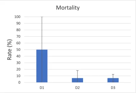
When the trial ended, individuals from the first density (D1 = 6 kg.m-3) presented an
average mortality rate (±SD) of 50 ± 50% whereas individuals from the second (D2 = 15 kg.m-3) and third (D3 = 30 kg.m-3) densities presented similar mortality rates of 6.67
±11.55 % and 6.67 ± 5.77%, respectively (Fig 4.2.2).
0 10 20 30 40 50 60 70 80 90 100 D1 D2 D3
R
at
e
(%)
Mortality
Fig 4.2.2 - Mortality rate of Holothuria forskali according to the different densities in question at the end of the trial (D1 = 6 kg.m-3; D2 = 15 kg.m-3; D3 = 30 kg.m-3).
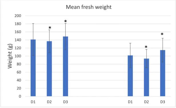
The remaining surviving individuals presented a decrease in mean fresh weight when compared to the initially determined mean fresh weight. Individuals from D1 went from a mean fresh weight (±SD) of 141.14 ± 39.74 g to 101.71 ± 30.31 g (a loss of 27.94%), individuals from D2 went from a mean fresh weight (±SD) of 137.07 ± 28.17 g to 93.68 ± 22.70 g (a loss of 31.66%) and individuals from D3 went from a mean fresh weight (±SD) of 148.63 ± 32.51 g to 114.90 ± 29.45 g (a loss of 22.70%).
22
Individuals from D2, as well as individuals from D3, presented statistically significant differences before and after the trial in accordance with a One-Way ANOVA [F(5, 90) =
7.850; p < 0.001] followed by a Pairwise Multiple Comparison Procedure (Tukey; p < 0.001), while individuals from D1 presented no statistically significant differences between the same interval (Fig 4.2.3), however there were no statistically significant differences between any of the individuals in captivity according to the same test.
0 20 40 60 80 100 120 140 160 180 200 D1 D2 D3 D1 D2 D3
W
eigh
t
(g)
Mean fresh weight
Fig 4.2.3 - Mean fresh weight (±SD) in individuals of Holothuria forskali in the beginning (January) and the end (May) of the trial (D1 = 6 kg.m-3; D2 = 15 kg.m-3; D3 = 30 kg.m-3). *Statistically significant differences between
January (trial onset, Left) and May (trial end, Right).
Based on the initial baseline group (t0 = 88.61 ± 14.38 g), there was also a loss in terms
of mean gutted weight with individuals in captivity (D1 = 56.35 ± 19.42 g; D2 = 58.84 ± 11.21 g; D3 = 70.86 ± 13.47 g) showing significant differences with the initial t0 group
according to a Kruskal-Wallis [H(3) = 18.851; p < 0.001] followed by a Pairwise Multiple
Comparison Procedure (Dunn; p < 0.001), however there were no significant differences of mean Gutted weigh between any of the individuals in captivity according to the same test (Fig 4.2.4).
*
*
*
23 0 20 40 60 80 100 120 t0 D1 D2 D3
W
eigh
t
(g)
Mean gutted weight
Fig 4.2.4. - Mean gutted weight (±SD) in individuals in the beginning (January) and at the end (May) of the trial (t0 = Baseline group; D1 = 6 kg.m-3; D2 = 15 kg.m-3; D3 = 30 kg.m-3). *Statistically significant differences
between January (trial onset) and each May group (trial end).
With both the gutted weight and fresh weight it was then possible to determine the relative available mass in each sea cucumber after dividing their individual gutted weight by their individual fresh weight. This in turn can translate how much of the sea cucumber, when paired with the gonadossomatic index, is viable for regular human consumption and how much of its weight is unnecessary padding (i.e. unconsumable organs, such as respiratory trees and Cuvierian tubules or excess water and stomach content).
From the following data regarding the mean relative available mass (Fig 4.2.5), there were no statistically significant differences between the baseline group (t0 = 52.44 ±
4.86 %) and any of the individuals in captivity (D1 = 56.78 ± 6.06 %; D2 =60.38 ± 3.19 %; D3 = 60.18 ± 3.90 %) in accordance with a Kruskal-Wallis [H(3) = 7.415; p = 0.060].
*
*
24 0 10 20 30 40 50 60 70 t0 D1 D2 D3 Wild Gu tt ed w eigh t/ Fr esh w eigh t (%
)
Mean relative available mass
Fig 4.2.5. - Mean relative available mass (±SD) of individuals in the beginning (January) and at the end (May) of the trial (t0 = Baseline group; D1 = 6 kg.m-3; D2 = 15 kg.m-3; D3 = 30 kg.m-3).
Regarding the Gonadossomatic Index (GI), the only significant difference noted was between the mean percentage (±SD) in the wild individuals from May (Wild = 0.83 ± 0.70 %) and every other group (t0 = 18.85 ± 6.06 %; D1 = 17.98 ± 10.33 %; D2 = 12.27 ±
7.92 %; D3 = 13.48 ± 7.89 %) according to a Kruskal-Wallis [H(4) = 39.238; p < 0.001]
followed by a Pairwise Multiple Comparison Procedure (Dunn; p < 0.001). No difference was presented between the initial t0 group and any of the different captivity groups or even
25 Fig 4.2.6 - Variation of mean gonadosomatic Index (±SD) in Holothuria forskali in the beginning (January) and at the end (May) of the trial (t0 = Baseline group; D1 = 6 kg.m-3; D2 = 15 kg.m-3; D3 = 30 kg.m-3; Wild = Wild
individuals collected at the end of the trial). *Statistically significant differences between each group and wild individuals in May (trial end).
4.3. Histological analysis
From the histological analyses it was possible to accurately determine the sex ratio of the individuals within this trial. Overall there was a prevalent majority of females over males, with the initial t0 group being comprised of 80% females, 20% males and no undetermined
individuals (without identifiable gonads). The smallest stock density studied, D1, presented an absolute prevalence of females (100%). The remaining stock densities presented a more balanced sex ratio, with D2 being comprised of 63.33% females, 21.67% males and 15% undetermined individuals and D3 being comprised of 47.04% females, 31.85% males and 21.11% undetermined individuals, making it the most balanced of the stock densities in question when it comes to sex ratio. In total, female holothurians comprised nearly 2 thirds (66.39%) of the sea cucumbers at the end of the trial, while males took up a little over one fifth (20.07%) and undetermined individuals were close to one sixth (13.54%) as seen in the figure below (Fig 4.3.1).
26 0 10 20 30 40 50 60 70 80 90 100 t0 D1 D2 D3 Total
R
ela
tiv
e
Fr
eq
u
en
cy
(%
)
Male to Female ratio according to Stock Density
F M U
Fig 4.3.1 - Sex Ratio of Holothuria forskali according to Stock Density. (F) Female; (M) Male; (U) Undetermined. (t0 = Baseline group; D1 = 6 kg.m-3; D2 = 15 kg.m-3; D3 = 30 kg.m-3).
Upon inspecting the histological cuts under the microscope and classifying them under the stages established on chapter 3.3, the most abundant stage was Stage III (Fig 4.3.2 - C and D), with certain individuals showing signs of still being in Stage II (Fig 4.3.2 - A and B), and a sparse minority in Stage V (Fig 4.3.2 - E and F) as can be seen in figure 4.3.3. There were no individuals at Stage I or at Stage IV.
Following a two-sided Fisher test with Freeman-Halton extension, there were no statistically significant differences in the proportions of maturity stages between any of the densities in question in either the males (p = 0.629) or the females (p = 0.196).
27 Fig 4.3.2. - Microscopic images of different gonadal stages in Holothuria forskali. (A) Growing stage on a female individual; (B) Growing stage on a male individual; (C) Mature stage on a female individual; (D) Mature stage on a male individual; (E) Post-Spawning stage on a female individual; (F) Post-Spawning stage on a male individual. (DO) Developing Oocyte; (GW) Gonadal wall; (L) Lumen; (MO) Mature oocyte; (RO) Relict oocyte; (Sc) Spermatocyte; (Sz) Spermatozoa.
MO L Sc GW GW Sz DO
C
D
E
F
A
B
L GW GW GW GW Sz Sz L L MO MO RO28 Fig 4.3.3 - Relative frequency of each developmental stage recorded in the sampled male (M) and female (F) individuals according to their different stock densities (t0 = Baseline group; D1 = 6 kg.m-3; D2 = 15 kg.m-3; D3
= 30 kg.m-3).
After the optical analysis, female oocytes were then measured and had their mean diameter determined (Fig 4.3.4). Individuals from D2 presented a mean oocyte diameter of 105 ± 22 μm, a statistically significant smaller mean oocyte diameter than individuals from the highest density (D3 = 112 ± 21 μm), as well as individuals from the initial baseline group (t0 = 111 ± 19 μm), in accordance with a One-Way ANOVA [F(3, 871) = 7.017; p <
0.001], followed by a Pairwise Multiple Comparison Procedure (Tukey; p < 0.001). Individuals from the smallest density (D1 = 106 ± 15 μm) presented no statistically significant differences with any of the other groups.
0 20 40 60 80 100 120 140 t0 D1 D2 D3 Size (μm)
Mean oocyte diameter
Fig 4.3.4 - Mean oocyte diameter registered in individuals according to their different stock densities (t0 =
Baseline group; D1 = 6 kg.m-3; D2 = 15 kg.m-3; D3 = 30 kg.m-3). *Statistically significant differences between
each group and individuals from D1.
29
Regarding the oocytes’ relative frequency, the t0 group presented a relative majority
(33.56 %) of oocytes of sizes between 117-131μm, followed by D3 and D1 with a relative frequency of 26.57 % and 25.56 % of oocytes in the same size interval, respectively. All individuals from captivity (D1, D2 and D3) presented a relative majority of oocytes of sizes between 103-117 μm, with D2 having the smallest relative frequency (29.26 %), followed by D3 (30.63 %) and lastly D1 with the most relative frequency of oocytes of that size interval (38.89 %). Despite this reasonable difference in frequency, D1 presented no oocytes bigger than 145 μm, whereas D2 presented a number of oocytes as big as 173 μm and D3 even goes further with oocytes as big as 188 μm (Fig 4.3.5).
Fig 4.3.5 - Length and relative frequency of female oocytes in sampled Holothuria forskali (t0 = Baseline group;
D1 = 6 kgm-3; D2 = 15 kgm-3; D3 = 30 kgm-3) with moving average trendline (Red).
0 10 20 30 40 60 74 88 103 117 131 145 159 173 188 R e la ti v e Fr e q u e n cy ( % ) Oocyte Size (μm)
T0
0 10 20 30 40 60 74 88 103 117 131 145 159 173 188 R e la t iv e F r e q u e n c y ( % ) Oocyte Size (μm)D1
0 10 20 30 40 60 74 88 103 117 131 145 159 173 188 R e la ti v e F re q u e n cy ( % ) Oocyte Size (μm)D2
0 10 20 30 40 60 74 88 103 117 131 145 159 173 188 R e la t iv e F r e q u e n c y ( % ) Oocyte Size (μm)D3
t0
30
4.4. Lipid content
As for the total lipid content, there were no statistically significant differences between the mean (± SD) lipid content any of the tested groups (t0 = 0.71 ± 0.13 %; D1 = 1.16 ± 0.11 %;
D2 = 1.18 ± 0.34 %; D3 = 0.98 ± 0.17 %; Wild = 0.92 ± 0.17%) in accordance with a One-Way ANOVA [F(4, 10) = 2.810; p = 0.084], despite t0 presenting a seemingly smaller
average lipid content than the rest (Fig 4.4.1).
Fig 4.4.1 - Total Lipid content present in sampled muscle tissue of Holothuria forskali in the beginning (January) and at the end (May) the trial (t0 = Baseline group; D1 = 6 kgm-3; D2 = 15 kgm-3; D3 = 30 kgm-3; Wild
= Wild individuals collected at the end of the trial).
4.5. Protein Content
Regarding the total protein content, much like the previous analysis, there were no significant differences that could strongly justify the variance in mean (± SD) protein content in any of the individuals in the trial (t0 = 5.91 ± 1.25 %; D1 = 5.75 ± 0.52 %; D2 =
5.84 ± 0.38 %; D3 = 6.11 ± 0.65 %; Wild = 5.43 ± 1.45 %) according to a Kruskal-Walis [H(4) = 0.294; p = 0.990], as demonstrated in figure 4.5.1.
31 Fig 4.5.1 - Total protein content present in sampled muscle tissue of Holothuria forskali in the beginning (January) and at the end (May) of the trial (t0 = Baseline group; D1 = 6 kgm-3; D2 = 15 kgm-3; D3 = 30 kgm-3;
Wild = Wild individuals collected at the end of the trial).
5. Discussion
This study aimed to determine the effects of different stock densities on the rearing of
Holothuria forskali in captivity, as well as during transport. This represents a step forward
towards the optimization of aquaculture techniques regarding this species, from capture all the way to broodstock maintenance in captivity.
5.1. Capture, transport and acclimation
Capture and transport can both induce sharp levels of stress upon the collected individuals (Purcell et al, 2006). The captured specimens must therefore be carefully handled in order to mitigate whatever negative aspects may come from these situations (Santos, 2017).
Holothuria forskali is known to be able to recover after stressful conditions (Tonn et al,
2016), much like most species of holothurians (Agudo, 2006; Dolmatov & Ginanova, 2009). However, while individuals collected in January were able to acclimate to captivity conditions without trouble, similar to what has been reported by Santos (2017) under the
32
same transport protocol, specimens collected in December failed to meet those standards. Individuals from December sampling campaign revealed a more adverse reaction to handling than individuals collected in January, with a higher rate of Cuvierian tubules’ release, evisceration and even mortality. With both campaigns following the same capture and transport protocol, the most notable difference between the two is the lower stock density during transport and acclimation in January. With this in mind, lower stock densities through transport and acclimation period seem to indicate better results for individuals of Holothuria forskali and are therefore recommended for future aquaculture studies regarding holothurians. The same recommendations are applicable to aquaculture rearing with economic interest.
5.2. Body mass and mortality rate
Regarding the trial itself, the most glaring difference between the densities in question was the seemingly larger mortality rate present in D1 when compared to the other two densities. However, this difference doesn’t seem to be originated from any morphological difference between the densities studied or the water parameters between systems, but rather a difference in the original amount of sea cucumbers within each density. Due to its’ smaller size alongside the limited volume of the tanks available for the study, D1 ended up being supplied with only two sea cucumbers per tank, leaving the entire density in question to be represented by a total of two Holothuria forskali, with their corresponding replicates, as opposed to D2 and D3 which were represented by a total of five and ten holothurians, with their corresponding replicates, respectively. Looking at the entire mortality list, D2 presented the loss of one individual while D3 presented two, by themselves these casualties are not much different from D1 which presented a total loss of three sea cucumbers. The difference lies in the density’s representation, with far less holothurians to supply D1, the small casualty list ended up leaving a bigger impression than the other two densities which had a more robust representation (Landsberg & Sands, 2011). As such, the results pulled from D1 ended with a lack of representation, therefore making them less robust in certain aspects when compared to the other two densities. The sea cucumber’s ability to store and expel water from inside its own body makes it difficult to accurately assess the weight of individuals, often leading to high variability in
33
fresh weights (Prescott et al, 2015). In order to reduce such variability, the weighting procedure was standardized to establish valid comparisons. Following a methodology based on this principle, it’s clear from Fig 4.2.3. and Fig 4.2.4 that there was a loss in terms of both mean fresh and gutted weight in all individuals in captivity without exception. This loss in weight could result from the individuals’ lack of variety in diet throughout the trial (Battaglene, 2002) or a lack of debris in abundance and other benthic organic matter (Ceccarelli et al, 2018; Gao et al, 2011).
All densities in question presented a loss of mean fresh weight of around 20-30% (D1 = 27.94%, D2 = 31.66% and D3 = 22.70%), although not a positive outlook from an aquaculture perspective, individuals from this trial still present an improvement over previous studies where certain species of sea cucumbers, including Holothuria forskali, presented a loss of mean fresh weight of around 36-40% (Morgan, 2007; Santos, 2017).
Despite the losses in both fresh and gutted weight, there were no differences regarding the mean relative available mass (how much of the sea cucumber is available for regular consumption, except the gonads) in each stock density. All individuals in captivity showed no differences with the individuals sacrificed at the beginning of the trial, which, in turn, points towards the loss in biomass to have affected the entire animal and not just the tegument and muscle mass. In other words, if the loss in biomass had merely affected the gutted weight then there should have been a parallel decrease in the mean relative available mass, however with the proportional decrease in mean fresh weight the amount of sea cucumber available for regular consumption remains unchanged.
With no considerable differences regarding the amount of sea cucumber for human consumption, the most viable stock density from an economic perspective is the one which can hold the biggest amount of sea cucumbers, in this case D3 (30 kg.m-3).
Regarding the use of broostock for reproductive purposes, results point to D3 being the most suitable density to implement out of all the densities in this trial. Considering the lack of morphological differences between males and females in sea cucumber species, with no sexual dimorphism between individuals to determine their sex, the less intrusive solution for a successful spawning induction is having a higher number of individuals present (Pratas et al, 2017). As such, a higher density will have better chances of being consisted by both sexes, as corroborated by fig 4.3.1.