A Work Project, presented as part of the requirements for the Award of a Master Degree in Finance from the NOVA – School of Business and Economics.
Microstructural changes before Macroeconomic Announcements: Predictability of Economic Surprises in the U.S. market
Rita Dias Barreto Calçada 930
A Project carried out on the Master in Finance Program, under the supervision of: Afonso Eça
2 Abstract
Flow of new information is what produces price changes, understanding if the market is unbalanced is fundamental to know how much inventory market makers should keep during an important economic release.
After identifying which economic indicators impact the S&P and 10 year Treasuries. The Volume Synchronized Probability of Information-Based Trading (VPIN) will be used as a predictability measure. The results point to some predictability power over economic surprises of the VPIN metric, mainly when calculated using the S&P. This finding appears to be supported when analysing depth imbalance before economic releases. Inferior results were achieved when using treasuries.
The final aim of this study is to fill the gap between microstructural changes and macroeconomic events.
3 1. Introduction & Literature Review
The aim of this study is to understand if microstructural changes in specific assets before Macroeconomic data releases have predictive properties over the result of the release, mainly if they are able to predict positive or negative surprises.
The study starts by understanding which macroeconomic announcements produce a stronger impact on the financial markets. Subsequently, focusing on those announcements, predictability tools to forecast if the results deviate from the expectation are developed. Lastly, with all the knowledge acquired an investment strategy is developed.
The motivation for this study is to fill in the gap between the studies of informed trading and its applicability to days with macroeconomic releases. The reason why this study is focused on United States macroeconomic events is due to their importance across the globe as a gauge to measure the wealth of the financial markets as well as the current Monetary Cycle. As Europe and most of the developed countries are following some sort of Quantitative Easing, expansionist policies might bias the results of the data releases. Moreover, the Federal Open Market Committee, section of the United States Federal Reserve that decides the monetary policy to be followed, is constantly monitoring the employment, nonfarm payroll and other macroeconomic data, making the data releases so important to signal the monetary policy.
In the financial markets, price changes are usually driven by flow of information. Easley et al. (1992) discovered that an increased inflow of new information reduces the time between trades, and the more relevant the news the more volatility it attracts. For this reason, there has been a number of studies that try to identify informed traders. The concept of informed traders might be misinterpreted as traders with inside information. However, that would be a misspecification. Bouchaud et al. (2009), developed an interesting definition of informed trader as a trader that is able to earn profit above transaction costs. It is clear that this definition does not imply the presence of inside information.
4
In this case, an informed trader might be someone who is able to better interpret economic news and generate profit from it. Cenesizoglu, Dionne & Xiaozhou (2014), showed that between the release of economic surveys and announcements there is still a significant flow of information that can be used by traders. Another evidence of informed trading would be the Flash Crash of 6 May 2010. This events make it imperative to try and predict informed trading. The increasing number of studies that conclude that economic surprises produce an impact on several different assets is what motivates this study. Amongst others, Balduzzi et al. (2001), try to understand the impact that economic releases have on US Treasuries. Using the microstructure properties of the Bond market, such as trading volume, bid-ask depth and its spread. They found that public news explains a substantial amount of the volatility that follows the announcement and that adjustments are usually corrected within one minute. This analysis was done to four tenors, 3 months, 2, 10 and 30 years. Even though there are indicators that impact all the maturities almost evenly it is clear that the largest the maturity the largest the impact. Reason why in this study a longer maturity is evaluated.
Andersen et al. (2002) connect high-frequency dynamics to fundaments by concluding that many U.S. announcement surprises produce conditional mean jumps on exchange rates. Moreover, they found that there is an asymmetric impact of news; bad news seems to have a stronger impact compared to good news. This conclusion is interesting, as throughout this study the model appears to have a stronger explanatory power over bad news rather than good news.
This paper relates to these previous studies in some interesting points, but it also deviates in relevant aspects. Both Andersen et al. (2002) and Balduzzi et al. (2001) appear to arrive to the conclusion that macroeconomic announcement such as payrolls, employment and durable goods produce the largest significant impact on the price of exchange rates and bond markets. Despite finding most of the same announcements relevant, it also finds that Retail Sales and Manufacturing PMIs, amongst the announcements with the highest impact; however, the
5
explanatory power seems to be relatively lower than the referenced studies. Opposite to most studies, the aim is to go further and to try and connect order flow to predict news.
Although there is substantial literature about the impact of macroeconomic news to microeconomic aspects of several assets, mainly Treasuries and Exchange Rates. Few studies try to predict the macroeconomic release. Rime, et al. (2010) gives a step in this direction, finding tools to predict movements in the exchange rates. Using the data of one year for 3 major exchanges, they find evidence to support order flow as a predictor of daily movements in exchange rates. Moreover, Pasquariello & Vega (2006) analyse the impact of private and public information in the price formation of U.S. Treasuries. They conclude that unexpected order flow leads to persistent changes in U.S. Bond prices both in days with and without economic releases. Also, the study reveals that the correlation between order flow and price changes is the highest when beliefs are dispersed and public announcements are noisy. Meaning, that the existence of several different beliefs is what seems to make the order flow central to price formation. Following the same line of Pasqiariello et al. (2006), days without relevant economic events are set as the benchmark. Understanding in which microstructural aspect does days with economic releases deviate from days without relevant announcements will help the development of the predictability tools.
Throughout this work order flow will be evaluated as a predictability tool. This study will use the Volume Synchronised Probability of Informed Trading (VPIN), developed by Easley, López and O’Hara (2010) as the central model to try and predict economic surprises.
The choice of this model fits the new developments in the financial markets, where almost all assets are exclusively traded through electronic platforms. High-frequency trading has become a considerable portion of the financial markets. The Securities and Exchange Commission in 2014 compiled a series of studies regarding HFT, where they conclude that the
6
average research found that more than 50% of the total volume of the US equities are HFT. It is assumed that for the Futures market this value is even greater.
This study will focus on order imbalances. When the order flow is unbalanced, market makers might be adversely selected and face possible losses. They try to predict order toxicity in order to manage their inventory position. Orders were defined by Easley et al. (1996) as “toxic when they adversely select market makers, who may be unware that are providing liquidity at a loss”. If the market makers believe that the flow toxicity present in the market is too strong, they will liquidate their positions. This process usually happens before relevant macroeconomic announcements, liquidity disappears from the market as liquidity providers are unsure if there are traders with more information than them.
Furthermore, the motivation to use this model relates to the fact that several studies have found that the VPIN could be used as a predictability tool of large movements in the financial markets, such as the flash crash. Easley et al. (2011). By analysing the S&P future contract, they found evidence that minutes before the Flash Crash, the VPIN metric reached the highest level in the history of the contract. Finally, in the same study they compare the VPIN to the VIX as predictability measures. They found that although the VIX increased before the crash it only reached its pick after the market collapsed. So, it is possible to conclude that the VIX was impacted by the flash crash producing no explanatory power over it, whereas the VPIN appeared to have some predictability information.
The VPIN metric departures from the Probability of Information-Based Trading (PIN) Model developed by Easley et al. (1996). This metric follows the basic principle that trading is an exchange between liquidity providers and position takers.
The PIN model has a few drawbacks for the dataset that is going to be used. Firstly, the PIN model is a daily measure of Probability of Informed Trading. Since macroeconomic releases occur throughout the day, only the hours around economic releases will be studied to understand
7
if they provide some predictive power. Moreover, by using high-frequency data, the trading time is not continuous, as there are seconds with a large flow of orders and others where there are no trades at all. For this reason, the VPIN model will be studied, as it is not only able to analyse high-frequency data, but also is able to divide the sample in time volume buckets. Ané & German (2000) had already developed this method that defines trade time as volume increments. The concept of volume time bucket is explained further. Another reason why the volume buckets are so appropriate for this type of data is that it is able to deal with volatility clustering that is a characteristic of high frequency data. Thus, as significant movements in price are usually attached to increasing trading volumes, it is a way to sample by volatility, normalize and reduce heteroscedasticity.
The main focus of this study is to use the VPIN as the main predictability measure of economic data releases; however, other microstructure properties such as the depth of the first level of the order book and bid/ask spread might have predictability information.
Several studies analyse bid-ask metrics, such as the bid-ask depth imbalance and spread; these metrics serve as a liquidity and predictability proxies. Rühl & Stein (2014), concluded that the bid-ask spread has two components, volatility (measures risk) and information component (predictability element). Zheng, Moulines, & Abergel (2013), concluded that the conditional probability of the next trade sign is severely correlated with a bid-ask depth imbalance metric. In this study the depth imbalance (DI) will be evaluated in order to see if combined with OI creates an improved predictability tool. Xu, J., (2013) defines DI as a metric that is able to capture the liquidity pressures of the limit order book, the same DI metric will be used in this study; Zhan, et al. (2008) highlight possible drawbacks of the DI metric; in their study they conclude that the bid ask depth reflects the liquidity that marker makers are willing to provide after taking into account the market order flow. This conclusion might indicate that the addition of information contained in the DI is already accounted in the OI.
8
The remainder of the work is organized as follows. Section 2 presents the data set; section 3 describes the methodology, first for the selection of the major economic events, later the model to predict surprises. Section 4 provides the results and discussion. Section 5 concludes.
2. Data
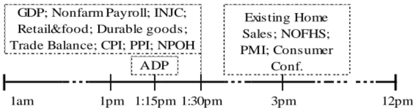
The data used for the expected and realized value of the macroeconomic data was provided by Bloomberg. The forecasts correspond to the median of all the predictions attained by Bloomberg. Time table 1 highlights the time of the announcements.
Figure 1: Time of economic releases (GMT)
For the initial analysis of the impact of surprises on prices of the S&P Future and 10 year Treasuries, minute bar data will be used. For the S&P 500 the data set starts on the 30th of September 2007. Whereas, the Treasury data starts on the 10th of June of the same year. They both end in the end of March 2015. Tick data is used for the subsequent analysis.
Tick data displays the information of transaction volume and price, best bid and depth, best ask and depth to the closest second. The sample covers the period from 3rd of April 2015, until the 23rd of November from 7am until 12am EST time, as most economic releases occur between 8 and 10am. The tenor chosen for the U.S. Treasuries was 10 years because it is the one that combines both highest duration with highest liquidity, prevailing above 5 year and ultra-bonds. Lastly, the available data was divided in two. From the 3rd of April until the 31st of August
an in-sample analysis is produced (referenced as in-sample data). From the 1st of September onwards the data will be used to test all the knowledge acquired (out-of-sample data).
3. Methodology
Firstly, to try and predict announcement news, one must understand which news have the highest impact on both the S&P 500 and 10 year treasuries. To make all the economic variables
Existing Home Sales; NOFHS; PMI; Consumer Conf. 12pm 1:15pm ADP GDP; Nonfarm Payroll; INJC; Retail&food; Durable goods; Trade Balance; CPI; PPI; NPOH
9
comparable, the same methodology of Balduzzi et al. (2001) and Andersen et al. (2002) is used in order to standardize news. The surprise for each k indicator at time t is divided by its sample standard deviation. As represented below.
𝑆𝑘𝑡 =
𝐴𝑘𝑡−𝐸𝑘𝑡
𝜎̂𝑘 (1)
where 𝐴𝑘𝑡 represents the value of the economic indicator k at time t, 𝐸𝑘𝑡 corresponds to the
median of the predicted values, and 𝜎̂ is the sample standard deviation of the difference 𝑘
between actual value and predicted. Contrasting both referenced studies, the standard deviation is calculated in a rolling basis, using the past 20 days. This was done so that the standard deviation does not include forward looking information and so it does not incorporate completely different economic cycles that could produce a bias to this metric.
In order to assess the impact of economic surprises on the price on the future of the S&P500 and on the 10 year U.S. Treasuries, this simple OLS regression was computed
∆𝑃𝑡−1:𝑡+𝑥,𝑘= 𝛽0+ 𝛽1∙ 𝑆𝑘𝑡+ 𝜀𝑡 (2)
where ∆𝑃𝑡−1:𝑡+𝑥,𝑘 corresponds to the price change of each asset between the end of the minute prior to the announcement until 1, 5,15 and 60 minutes after for the kth indicator (k=1,...,14).
Andersen et al. (2002) simply defined VPIN as the rolling average of the absolute Order Imbalances. In spite of this simple definition, several steps must be taken, illustrated below.
Figure 2: Steps to calculate VPIN
time
T3 T4
Bucket #1 Bucket #2 Bucket #3 vol trade 1 vol trade 2 T5 T6 vol trade 7 vol trade 8 vol trade 9 *if makes price go down *if makes price go up
Step 2: Within each bucket, define each trade as buyer or seller initiated
Step 3: Calculate OI for each bucket. VPIN is just na average of the last 'x' OI
Buyer Initiated
Seller Initiated Step 1: Divide the sample in vol buckets
0 0,5 1 0 50 100 150 200
Buy Initi ated Sell Init iat ed
Vol OI VPIN (2 Buckets) trade trade trade trade trade trade trade trade trade
10
Tick data provides granular information on trades, changes in bid-ask price and depth. Nevertheless, there are also some drawbacks from using this type of data. Tick data captures each trade and each change on bid-ask, which means that it is not a stationary series. There are seconds/minutes with much higher market flow than others, making them incomparable. For this reason, a different time metric is computed – volume buckets. Allowing for this change enables comparisons between buckets within one day or even between different days. To construct volume buckets, it is necessary to decide how to divide each day. In this case the future of the S&P has an average morning volume of 554,718.01. In order to divide each morning in 40 intervals (# buckets per morning = B), each bucket of time should have on average 13,868 trades. In the case of the 10 year treasury futures with an average morning volume of441,393.93, each morning will be divided on average in 15 buckers, each having an average volume of 29,426 trades. The value of B will be explained further in the results section. Identical to previous VPIN studies, the average volume of trades during the morning is the average over the whole in-sample period. Subsequently, this methodology leads to a forward looking bias in-sample. Nevertheless, all these values will be used to calculate the VPIN out-of-sample. A rolling window would not be appropriate in this case, as the objective is to compare each trading volume to a consistent metric. Even though there are month with much lower trading volume, like June in the case of the Treasuries, this does not necessarily mean lower probability of informed traders in a specific time frame. The summary of this analysis can be seen in appendix 3. Just like in Andersen et al. (2013), these graphs highlight the need to “detrend” the volume of trades to make them comparable.
When trading intensity increases, the time to fill in a volume bucket is lower than when trading is slow. This is why volume buckets provide such a good comparison tool.
After dividing the sample in volume buckets it is necessary to understand which trades are buyer or seller initiated. There has been an increasing amount of discussion on this topic.
11
Chakrabarty et al. (2014) presents an interesting discussion about the best methodology to classify trades, comparing the Bulk Volume Classification (BVC), used in this paper with the tick rule (TR) and Lee-Ready (LR) algorithm. In their study they compare the real trade classification provided by the NASDAQ Exchange with these metrics. They conclude that on the majority of the tests, the BVC classification is outperformed by the other. Nevertheless, the LR procedures is only reliable if level II information (order book data) mid quote is available and is reliable, as tick data is used the most appropriate method to classify trades will either be the same used by Easley et al. (2012) and Abad, D., and Yagüe, J., (2012), the BVC or the tick rule. Both methods will be tested, and ultimately, the one that appears to better explain surprises will be used. The TR is the simplest classification method, it classifies a trade as buyer-initiated if the current trade price is above the prior, and seller-initiated if it is below. If between two trades the price does not change, the classification will be the same as the previous.
On the other hand, to proceed with the BVC method, trades are aggregated over short periods, one minute intervals (in this case), then the standardized price change between the beginning and end of each interval is used to determinate the percentage of buy and sell orders. Using the same variables as Easley et al. (2012), the buy (𝑉𝑖𝐵) and sell (𝑉𝑖𝑆) are calculated as
𝑉𝑖𝐵 = 𝑉𝑖 ∙ 𝑍 ( 𝑃𝑖−𝑃𝑖−1 𝜎∆𝑃 ) (3) 𝑉𝑖𝑆 = 𝑉𝑖 ∙ [1 − 𝑍 (𝑃𝑖−𝑃𝑖−1 𝜎∆𝑃 ) ] = 𝑉 − 𝑉𝑖 𝐵 (4)
where 𝑉𝑖 is the volume traded in the time period 𝑖 − 1 to 𝑖. 𝑃𝑖− 𝑃𝑖−1 is the price change between that period, 𝜎∆𝑃 is the estimate standard deviation of price over in-sample. Z is the CDF of the
standard normal distribution. This method divides the trade between buyer and seller initiated, if there is no price change the volume is equally divided. If the price increases, the volume is mainly transferred to the buy rather than the sell; the opposite if price decreases.
12 𝑉𝜏𝐵= ∑ 𝑉 𝑖𝐵 𝑡(𝜏) 𝑖=𝑡(𝜏−1)+1 ; 𝑉𝜏𝑆 = ∑ 𝑉𝑖𝑆 𝑡(𝜏) 𝑖=𝑡(𝜏−1)+1 (5)(6)
where, 𝜏 corresponds to a bucket and t(𝜏 − 1) is the minute of the start of the bucket, and 𝑡(𝜏) the last minute of bucket 𝜏.
The final step before calculating the VPIN, is to compute the order imbalance (OI) of each volume bucket, which is simply the absolute difference between the buy and sell volume. It can be mathematically expressed as
𝑂𝐼𝜏 = |𝑉𝜏𝐵− 𝑉𝜏𝑆| (7)
Finally, to calculate the VPIN metric it is necessary to combine the order imbalance with the average trade volume during the morning and with the span that the VPIN metric is going to be evaluated. Mathematically the VPIN flow toxicity metric is
𝑉𝑃𝐼𝑁 =∑𝑛𝜏=1|𝑉𝜏𝐵−𝑉𝜏𝑆|
𝑛𝑉 =
∑𝑛𝜏=1𝑂𝐼𝜏
𝑛𝑉 (8)
Through this expression it is possible to understand that the VPIN metric is recalculated after each bucket and it only starts in the nth bucket. If n was equal to B (number of buckets per
day on average), there would be on average one value of VPIN per morning. As the aim of this study is to understand the Volume of Informed trading before the announcement, n has to be low enough so that on average there are enough buckets filled before the announcement.
The value of B will differ for Treasuries and for the S&P. Since the volume transacted, the type of agents that make up the bulk of the trades and the announcements evaluated for each assets differ. B and n will be sets so that each VPIN metric better captures the surprises. The results and comparison of several different parameters will be explained further. Nevertheless, for the S&P future, n will be set to be equal to 1 and B equal to 40. Making some simple calculations, since the analysed period is between 7:30am and 11:30am EST, 4 hours, each bucket would capture on average 6 minutes, allowing for 9 values of the VPIN before the announcement. In the case of the 10 year Treasuries, B will be set to 15 and n to 1, enabling on average 3 values of the VPIN before the earliest announcements.
13
After understanding which announcements to analyse and developing a metric of informed trading, a series of comparisons between the benchmark and days with relevant economic indicators like the average VPIN value and number of buckets during the day are calculated. These are simple metrics but highlight the difference between these days.
Finally, to try and predict surprises two regressions are analysed. First, to try and understand the explanatory power of news the following regression is analysed
𝑆𝑡 = 𝛽0+ 𝛽1∙ 𝑉𝑃𝐼𝑁𝑡−1+ 𝜀𝑡 (9)
where, 𝑉𝑃𝐼𝑁𝑡−1 is the last value of the VPIN right before the announcement. This means that
sometimes there will be no value of VPIN before the announcement, if trading intensity was low. On the other hand, when there is enough volume before the announcement, the last value of VPIN can be calculated only one minute before the announcement or several minutes before. This will depend on the amount of volume traded during the morning that will fill in the buckets. As there seems to be more explanatory power of the VPIN over negative surprises, a probit regression is analysed. The Probit provides some benefits over a normal OLS regression, as it tries to identify if the probability of a negative surprise increases with the value of VPIN. The regression has the expression below, and the variable will be defined as 0 if the surprise is above or equal to zero, and 1 other wise.1
𝑌𝑡 = 𝛽1 ∙ 𝑉𝑃𝐼𝑁𝑡−1+ 𝜀𝑡 (10) 𝑌𝑡= {0 𝑖𝑓 𝑆𝑡 ≥ 0
1 𝑖𝑓 𝑆𝑡 < 0
Using the second portion of the sample, an out of sample investment strategy is developed. By analysing the times when VPIN has some explanatory power over economic surprises, a threshold is defined, VPIN values above it should lead to negative surprises.
1 In order to decide between a probit and logit, the deviance metric was used. The deviance measures lack of fit, which means that a lowest value is preferred. In the case of the S&P the probit deviance was 33.072 and logit 33.041; for the treasuries was 48.9322 and 48.9468; As these values are so close to each other, both regressions appear to fit the data similarly, so it was chosen for simplicity to use the probit metric for both regressions. It is important to notice that for both regressions, the conclusions were the same.
14
Through the analysis of which economic announcements produce relevant impact, it is also possible to study the magnitude and sign of the impact. The sign will be crucial for the examination of the VPIN. If the signal is negative, the value of the standardized surprise will be the symmetric of the actual value. And this will substitute the value of 𝑆𝑡 in both equation (9) and (10) so that a “positive” new is expected to lead to positive returns.
Lastly, there are two dimensions that have to be evaluated. The predictive power of this methodology and the profitability of this strategy. For the former, the amount of predicted surprises over the total amount of announcements will be evaluated. For the latter, a simple return measurement of the strategy will be computed.
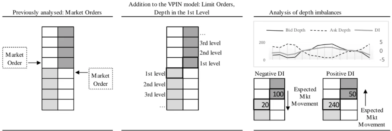
The focus of this study is to use the order imbalance, through the VPIN metric, as a predictability tool. Nevertheless, other levels of the financial microstructure will be studied to try and complement the VPIN. As illustrated in the figure below, whereas, VPIN analyses only market orders, DI is able to analyse a deeper level of the limit order book.
Figure 3: Difference between OI and DI, development of the DI tool
The same metric developed by Xu (2013) of DI will be used and it is represented below 𝐷𝐼𝑡= log(𝐷𝑒𝑝𝑡ℎ 𝐵𝑒𝑠𝑡 𝐵𝑖𝑑𝑡) − log(𝐷𝑒𝑝𝑡ℎ 𝐵𝑒𝑠𝑡 𝐴𝑠𝑘𝑡) (11) Opposite to the order imbalance, where the distribution is standardized by volume, in this case the data will be organized to the closest second.
After developing this additional metric, the same procedure as the one developed for the VPIN metric will be taken. First equation (9) will be computed for DI. Later, given the result
… 3rd level 2nd level 1st level 1st level 2nd level 3rd level 100 50 … 20 240
Previously analysed: M arket Orders
M arket Order
M arket Order
Analysis of depth imbalances Addition to the VPIN model: Limit Orders,
Depth in the 1st Level
Negative DI Positive DI -5 0 5 0 200
Bid Depth Ask Depth DI
Expected M kt M ovement Expected M kt M ovement
15
of this first analysis, an investment strategy will be developed and tested for predictability and profitability. When trying to understand the predictability power of the DI, the optimal number of seconds before the announcement is going to be evaluated in-sample and tested out of sample. Finally, both metrics will be combined in order to see if DI is able to add value to VPIN.
4. Results and Discussion
The initial step in this analysis is to identify and prove that it is interesting to predict economic surprises as they are predominant for the transfer of news and price formation. Regression (2) allows for this analysis. As mentioned in the introduction, this study starts with the premise that only flow of new information leads to price changes. Hence, the absolute value of the economic news release is irrelevant, only surprise will be studied.
In order to achieve robust conclusions, regression (2) will be computed for 4 different time frames, 1, 5, 15 and 60 minutes. Test in different time spans is fundamental; if the impact of a news surprise would happen only in the second after the release and then return to the initial value, there would be a great chance that the investor could not be able to sell at the pick/bottom, not profiting from knowing the surprise in advance.
The results are presented in appendix 1 and 2 for the S&P and Treasuries respectively. It is interesting to identify that the announcement surprise of some indicators are statistically significant for some time frames but stop being for others. This is specially the case for the S&P, i.e. Existing Home Sales and Initial Jobless Claims. Furthermore, regarding the S&P, the result that stands out the most is the decreasing R2 when the regression is done considering a longer time span. As previously mentioned, this initial analysis will allow the division of the sample in days with and without relevant economic releases. For the S&P the days with relevant economic releases will correspond to the days with ADP+, Durable Goods+, Manufacturing PMIs+, Nonfarm+ Payrolls, New One Family Households+ and Retail Sales+ (indicators with
16
highest R2). Neither, Existing Home Sales nor Initial Jobless Claims, will be incorporated in
this analysis as they combine to the lowest R2, with low significance levels at certain periods. For the Treasuries the results are slightly different, not only the announcements that appear to have a stronger impact vary, as there appears to exist a greater consistency in all the time frames. Hence, the days with relevant economic news will be the days with ADP-, CPI-, GDP-, Initial Jobless Claims+, Manufacturing PMIs-, Nonfarm Payrolls-, New One Family
Households-, New Privately Owned Housing- and Retail Sales-. It is important to notice that some of the announcements will have a positive and others negative impact over each asset, this is represented by a positive or negative sign over the indicator (+/-).
Prior to any further analysis it is necessary to look at different results and decide the value of the number of buckets per morning (B) and number of buckets to calculate VPIN (n) that lead to higher explanatory power (in equation (9)).
The VPIN metric works best if it is able to capture OI that deviate from the average. There has been no particular discussion on the correct value of B, it depends on what is being captured and on the trading frequency of each asset. If it is an asset that has a lot of trading volume throughout the morning, then B has to be higher. For this reason, the value of B for the S&P is higher than the value for the Treasures. Set to 40 and 15 respectively. As the aim of this study is to calculate possible small order imbalances that might reflect some information prior economic releases, B cannot be so small that is not possible to calculate a VPIN value before the economic release or to large that almost each trade is evaluated individually as the conclusions would be too unstable. The values were set to better accommodate the data that is being evaluated and this was done by regressing equation (9) several times until the best explanatory VPIN was reached (Analysis is represented in appendix 5).
Secondly, the variable that has the largest impact on the VPIN metric, is the value of n. As n increases some of the extreme order imbalances that might happened within a bucket can be
17
offset by averaging with the subsequent buckets, this is represented in appendix 3. VPIN will follow a log-normal distribution, meaning that the larger the variance the righter skewed will the distribution be. Appendix 4 illustrate that, as n decreases the distribution is increasingly more skewed, and these are the values that might be able to predict economic releases. Although the graphs are relative to the S&P the same applies to the Treasuries. As the purpose of this study is to try identify these extreme values and see if they can explain surprises, n should be as small as possible, so it is set to 1 in both cases.
As described above, there are two different metrics to classify trades that are applicable to the type of data used. Even though, several studies referenced above conclude that the BVC methodology is outperformed by other metrics, it appears that the VPIN metric calculated using the BVC metric has a stronger explanatory power over economic surprises. Using the parameters stablished before, the VPIN was calculated with both trade classifications. Making use of regression (9) it is possible to identify which metric has larger predictive power. As represented in appendix 6, the BVC classification appears to have a stronger explanatory power. Appendix 7 represent the distributions of both VPIN metrics. It is interesting to notice that Treasuries have VPIN spikes throughout the sample it seems that for the S&P they are more concentrated in the end period.
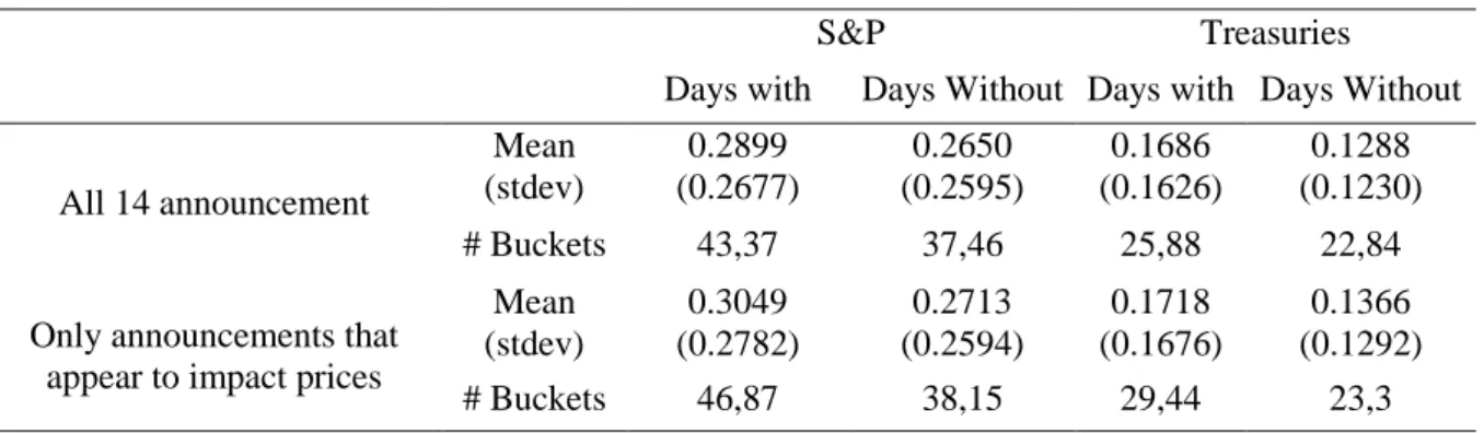
The first analysis is going to evaluate if the VPIN metric is able to identify if days with economic releases are days with more informed trading, presented in the table below.
Table 1: Comparison of the VPIN metric for days with and without relevant economic releases
S&P Treasuries
Days with Days Without Days with Days Without
All 14 announcement Mean (stdev) 0.2899 (0.2677) 0.2650 (0.2595) 0.1686 (0.1626) 0.1288 (0.1230) # Buckets 43,37 37,46 25,88 22,84
Only announcements that appear to impact prices
Mean (stdev) 0.3049 (0.2782) 0.2713 (0.2594) 0.1718 (0.1676) 0.1366 (0.1292) # Buckets 46,87 38,15 29,44 23,3
18
Overall, the average of the S&P distribution is higher, which represents that the order imbalances are usually stronger. When accounting for all the 14 analysed macroeconomic announcements, VPIN identifies on average an increased presence of informed traders than during the rest of the days. For the days with the chosen relevant economic announcements, this affirmation still holds, the average VPIN of the S&P and Treasuries is still higher than the benchmark. This initial conclusion is meaningfully, as it provides support for all the study. Providing evidence that during days with relevant economic releases there is a higher presence of informed traders. The fact that the average VPIN is higher on the days with relevant economic releases implies that the order imbalances throughout these days is higher. Which appears to corroborate with past studies of order imbalances as a source of information transmission, and crucial for price formation.
Moreover, days with relevant economic releases have a higher number of buckets that are filled. This means that these days attract a larger amount of traders which is interesting by itself and proves how relevant would be to predict economic surprises.
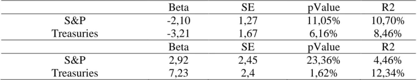
In order to understand if the VPIN has in fact explanatory power, the results of the regressions (9) and (10) will be evaluated.
Table 2: Result of equation (9) and (10) for the VPIN metric
Beta SE pValue R2 S&P -2,10 1,27 11,05% 10,70% Treasuries -3,21 1,67 6,16% 8,46% Beta SE pValue R2 S&P 2,92 2,45 23,36% 4,46% Treasuries 7,23 2,4 1,62% 12,34%
The table above represents the results of applying the VPIN to the economic surprises. It is interesting to see that, a higher value of VPIN in both seems to imply a future negative surprise. It is important to remember that each equation is done with the economic indicators that most affect the asset. Moreover, the VPIN metric appears to be statistically significant at 15% in the first equation of both assets. These are the most striking results of the paper as there indeed
19
appears to exist evidence, although small (small value of R-squared) that the VPIN metric has some explanatory power over future economic indicator releases.
To take this study even further, as there appears to exist evidence over the explanation of negative surprises, the second regression captures this effect. The probability of a negative surprise increases with the increase of the VPIN metric calculated for the Treasuries. However, the increase probability of negative surprise with increase VPIN of the S&P is not statistically significant. Strikingly, out-of-sample the S&P is a better predictor of negative surprises.
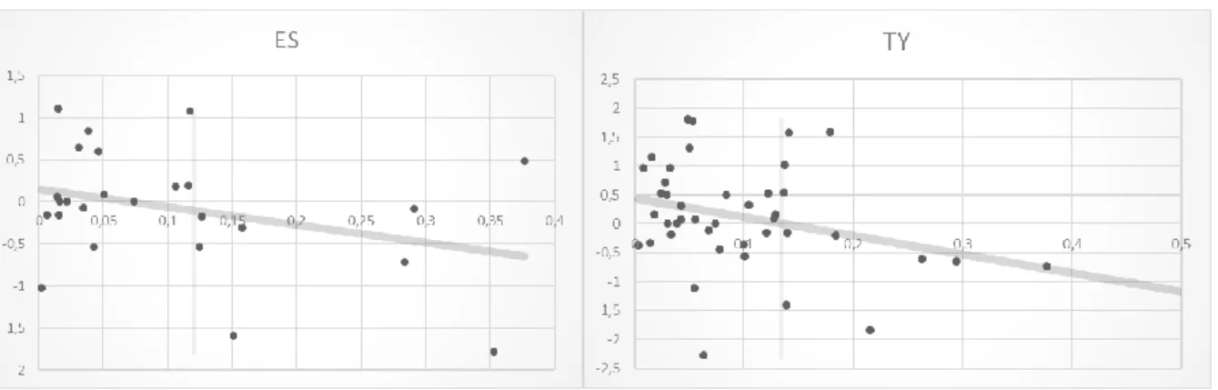
The final step is to identify a profitable investment strategy; the graphs below represent the distribution of VPIN to the future economic surprise.
Table 3: Graphical representation of regression (9) for both assets
For the S&P, values above 0.12 appear to be followed by negative surprises, whereas values below this threshold are usually followed by negative surprises. In sample, this threshold would have a percentage of correct signals of 73.91%. In the case of the 10 Year Treasuries, values above 0.13 appear to be followed by negative surprises and below by positive. Again, this threshold would have an accuracy of 65.85% in-sample. Given these results, these will be the thresholds analysed for the investment strategy that is developed out of sample.
These thresholds will be evaluated in two levels, first their predictability power, and secondly the profitability of this investment strategy. The first level conclusions are somewhat interesting, it seems that with the parameters defined above, the VPIN calculated for the S&P would be able to predict the news surprise with a 71.43% accuracy over 14 observations. On
20
the other hand of the scope, the Treasuries VPIN could only predict 56.52% (23 observations). A sensitivity analysis of the thresholds is displayed in appendix 8, it appears that the predictability power it is stable around these values. The profitability results of this strategy are presented below, two scenarios are analysed, if the position is liquidated after 5 or 60 minutes.
Table 4: Result of the Investment strategy given the specified threshold. In brackets is the Sharpe Ratio.
S&P 10 Year Treasuries
5 min -0,97% (-0,0840) -3,24% (-0,0156)
1 hour 1,63% (0,2507) 2,03% (0,0401)
For the level of risk that this strategy involves, even the risk reward for the treasuries is not substantially high (evaluated by the Sharpe Ratio); however, it is still interesting. Another interesting conclusion is that, although the S&P has a higher explanatory power, returns are still negative. Meaning that the predictability results should be used as an investment decision in other assets that might be influenced by these announcements, i.e. exchange and interest rates. To take this analysis further, and as in previous studies such as Easley et al. (2011), discovered that the VPIN appears to predict negative events, a new trading strategy is developed where the investor only invests if a negative surprise is expected (if VPIN is above the threshold). The results are presented in the table below.
Table 5: Result of the investment strategy of only investing in negative surprises
S&P 10 Year Treasuries
5 min 0,59% (0,0299) -0,08% (-0,0009)
1 hour 0,55% (0,1043) 0,65% (0,0250)
% correct 100% 42,86%
Interestingly, there is a 100% accuracy in predicting negative events, using the S&P, and returns are positive. The only drawback is that, there were only 4 values above 0.12, making this not a robust result. Though, it is curious that whereas the S&P profits and it is better at predicting negative surprises, Treasuries profit and predict better positive surprises.
Finally, the results from equation (9) for the DI analysis in-sample are presented in the table below. It is important to notice that even though several studies analyse the bid-ask spread, in
21
this time frame the value before the announcement does not deviate from the average, so it is not going to be evaluated.
Table 6: Result of equation (9) of the DI and evaluation of the metric out of sample
In-sample Out of sample
Beta SE pValue R2 % correct
S&P 0,17 0,12 17,77% 7,15% 31,25%
Treasuries -0,14 0,07 6,20% 7,22% 61,29%
Appendix 9 represents a sensitivity analysis of equation (9) when calculated for different seconds before the announcement. It is important to take into consideration that the highest R2 for the S&P was achieved when the variables were calculated 10 seconds before the announcement. Whereas for the treasuries the variables were calculated 25 seconds before. The most striking finding about these results, is even though the sign of the DI should reflect which side of the market is more probable of being depleted first. For the Treasuries, a greater volume in the bid side appears to predict a negative surprise. The opposite, more intuitively, happens within the S&P market, where a higher volume on the best bid (versus the best ask) appears to predict positive surprises. Hence, this might indicate a higher portion of informed traders in the S&P before the economic releases when compared to the Treasury traders. However, the S&P is only statistically significant at 17.77%.
Moreover, the predictability results are disappointing and do not appear to add value to the VPIN metric. When evaluating the signals, in the S&P, all the announcements except one, that the DI predicts so does the VPIN. For the Treasuries, there are some cases that DI correctly predicts when VPIN does not, however, the ones that VPIN predict offset that improvement. The comparison between signals is represented in appendix 10. Also, it appears that investing only when both metrics signal the same result does not improve the results in the S&P (correctly predicting only 57,14%), however it appears to slightly improve in the predictability for the treasuries (correctly predicting 66,67%). The only drawback is that the investor will most often restrain from being in the market. Investing only 6 out of 23 times.
22 5. Conclusion
There has been a number of studies that try to identify the impact of economic releases on several different assets, ranging from Treasuries, usually appointed as the assets that suffer more with changes in economic beliefs; Exchange rates, that similar to Treasuries incorporate the interest rate of the country in their pricing, making them exposed to new economic releases. And Equities that have a more indirect effect, but transmit the confidence that investors have over the overall economy of a country.
The aim of this study is to take a step further, given that positive and negative economic releases have significant impact on the S&P and 10 year Treasuries, the VPIN metric was be used to try and predict surprises. The first striking conclusion of this study is that on days with relevant economic events the existence of informed traders appears to be higher (higher VPIN). It appears to exist evidence that the VPIN has a small explanatory power over the economic surprises. Even though, in sample, the S&P has a smaller explanatory power, out of sample it appears to be a good predictor, mainly in the case of negative news. This conclusion corroborates with previous studies that use the VPIN to predict the flash crash.
Moreover, it is interesting to notice that opposite to the S&P, Treasuries have a stronger explanatory power over positive news rather than negative news. This is interesting, one of the reasons might be the fact that usually the aggregate of agents that participate on the treasury market are more risk adverse, not wanting to participate when expecting a negative surprise.
The final conclusion on this initial analysis is that the VPIN calculated relative to the S&P appears to have a stronger explanatory power given the chosen threshold, which means that it could also be given as a gauge to invest in other assets.
The poor returns of the S&P might be explained by the fact that, although the number is released at the exact time, there are also some specifications that come after the number that take longer to be analysed and may lead to a retracement of the price movement.
23
The final analysis of the bid-ask depth imbalance, is just the begging of a study that can be taken much further. Although the results were not enlightening, it was interesting to notice that for the S&P, a positive DI would be an indicator of a positive news. Whereas the opposite occurs in the Treasuries. This corroborates with the conclusion that the traders of the S&P are more informed.
Moreover, order imbalance appears to have a stronger explanatory power when compared to the depth imbalance. This corroborates past studies such as Zheng et al. (2013) where they study the long memory of the order flow. The rational is that when a trader resolves to buy/sell a considerable quantity of assets he may spit it into small pieces in order not to move the market and get a worse average price. Due to this mechanism, several studies recognize that previous market orders direction might be able to predict the next market order. This implies that order imbalance might have a larger explanatory power when compared to depth imbalance, as the first relates to market orders and the second to limit orders. Moreover, Zhan, et al. (2008), conclude that the DI captures the information that market makers attain from the order imbalance and make a decision to provide liquidity upon.
Finally, it would be interesting to explore further the bid ask structure of the assets, and be able to evaluate deeper limit order levels that might provide useful information. Nevertheless, and as concluded in this study it is important to notice that informed traders usually transmit new information to the market through market orders whereas limit orders are most often used by liquidity providers. This means that order imbalances and metrics that evaluate market orders should have a stronger explanatory power.
All in all, there are some interesting conclusions that open the desire to investigate more this subject, more types of assets, more levels of the limit order book, and different OI metrics. In 2015 there was also a new development in the VPIN metric advanced by Ke et al. (2015) that would be interesting for the next step in this analysis.
24 6. References
[1] Abad, David, and José Yagüe. (2012). “From PIN to VPIN: An introduction to order flow toxicity”. The Spanish Review of Financial Economics, 2: 74-83.
[2] Andersen, Torben G., Tim Bollerslev, Francis X. Diebold, and Clara Vega. (2003). “Micro Effects of Macro Announcements: Real-Time Price Discovery in Foreign Exchange”. American Economic Review, 93: 38-62.
[3] Andersen, Torben, and Bondarenko G Oleg. (2013). “Assessing Measures of Order Flow Toxicity via Perfect Trade Classification”. Unpublished.
[4] Thierry, Ané, and Helyette, Geman,. (2000). “Order Flow, Transaction Clock, and Normality of Asset Returns”. Journal of Finance, 55: 2259-2284.
[5] Balduzzi, Pierluigi, Edwin J Elton, and T Clifton Green. (2001). “Economic News and Bond Prices: Evidence from the U.S. Treasury Market”. Journal of Financial and Quantitative Analysis, 4: 523-543.
[6] Bouchaud, Jean-Philippe, J. Doyne Farmer, and Fabrizio Lillo. (2009). “How Markets Slowly Digest Changes in Supply and Demand”. Handbook of Financial Markets: Dynamics and Evolution, 57-160.
[7] Cenesizoglu, Tolga, Georges Dionne, and Zhou Xiaozhou. (2014). “Effects of the Limit Order Book on Price Dynamics”. Unpublished.
[8] Chakrabarty, B., Pascual, R., & Shkilko, A., (2014). “Evaluating Trade Classification Algorithms: Bulk Volume Classification versus the Tick Rule and The Lee-Ready Algorithm”. Unpublished.
[9] Easley, David, Nicholas, M., Kiefer, Maureen, O'Hara, and Joseph, B., Paperman, J. (1996). “Liquidity, information, and infrequently traded stocks”. The Journal of Finance. 51(4):1405– 1436.
25
[10] Easley, David, Marcos M., de Prado, and Maureen, O'Hara. (2012). “Flow Toxicity and Liquidity in a High-Frequency World." Review of Financial Studies, 25: 1457-1493.
[11] Easley, David, Marcos M., de Prado, and Maureen, O'Hara. (2011). “The Microstructure of the “Flash Crash": Flow Toxicity, Liquidity Crashes, and the Probability of Informed Trading”. Journal of Portfolio Management, 37 (2): 118-128.
[12] Easley, David, Marcos M., de Prado, and Maureen, O'Hara. (2012). “The Volume Clock: Insights into the High Frequency Paradigm”. Journal of Portfolio Management, 39 (1): 19-29 [13] Easley, David, and Maureen, O'Hara. (1992). “Time and the process of security price adjustment.”Journal of Finance, 47: 577–604.
[14] Ke, Wen-chyan, and Hsiou-wei William Lin, H.-w. W. (2015). “An Improved Version of the Volume-Synchronized Probability of Informed Trading (VPIN )”. Unpublished.
[15] Pasquariello, Paolo, and Clara, Vega. (2006). “Informed and Strategic Order Flow in the Bond Markets”. International Finance Discussion, 874.
[16] Rühl, R., Tobias, and Michael Stein. (2014). “Discovering and Disentangling Effects of US Macro-Announcements in European Stock Markets”. Unpublished.
[17]Rime, Dagfinn, Lucio Sarno, and Elvira Sojli. (2010). “Exchange rate forecasting, order flow and macroeconomic information”. Journal of International Economics, 1: 72-88.
[18] SEC. (2014). “U.S. Equity Market Structure Literature Review Part II: High Frequency Trading.” Staff of the Division of Trading and Markets March, 1-37.
[19] Xu, J. (2013). “Optimal Strategies of High Frequency Traders”. Unpublished.
[20] Zhang, Michael Yuanjie, Jeffrey R. Russell, e Ruey S. Tsay. (2008). “Determinants of bid and ask quotes and implications for the cost of trading”. Journal of Empirical Finance, 4: 656-678.
[21] Zheng, Ban, Eric Moulines, and Frédéric Abergel. (2013). “Price Jump Prediction in a Limit Order Book”. Journal of Mathematical Finance, 2: 242-255.
26 7. Appendix
Appendix 2: Impact of Economic Surprises on the Future of the 10 year Treasuries
Announcement
Beta P-Val R^2 Beta Pval R^2 Beta Pval R^2 Beta Pval R^2 1 - GDP 0,279 0,070 3,57% 0,248 0,237 1,53% -0,267 0,198 1,79% -0,362 0,264 1,35% Real Activity 2 - Nonfarm Payroll Employment 1,672 0,001 11,34% 1,984 0,000 13,23% 1,812 0,001 10,46% 1,410 0,028 5,15% 3 - ADP Employment Change 0,568 0,000 17,85% 0,608 0,000 14,58% 0,641 0,002 9,63% 0,915 0,002 10,01% 4 - Initial Jobless Claims -0,342 0,000 5,89% -0,404 0,000 4,32% -0,381 0,003 2,20% -0,162 0,364 0,20% 5 - Retail Sales 0,506 0,009 7,26% 0,701 0,005 8,36% 0,762 0,007 7,67% 0,734 0,035 4,72% Consumption 6 - Existing Home Sales 0,377 0,014 6,48% 0,291 0,225 1,61% 0,205 0,523 0,45% 0,158 0,750 0,11% 7 - New Privately Owned Housing 0,034 0,800 0,07% -0,131 0,413 0,73% -0,267 0,198 1,79% -0,362 0,264 1,35% 8 - New One Family
Houses Sold 0,451 0,004 8,87% 0,581 0,009 7,20% -0,008 0,982 0,00% -0,542 0,245 1,48% Investment 9 - Durable Goods Orders 0,272 0,031 5,13% 0,297 0,091 3,18% 0,315 0,131 2,55% 0,352 0,198 1,86% 10 - ISM Manufacturing PMI 1,394 0,000 27,57% 1,756 0,000 28,48% 1,610 0,000 17,03% 2,371 0,000 19,77% Net Exports 11 - Trade Balance 0,301 0,045 4,31% 0,236 0,177 1,97% -0,074 0,758 0,10% 0,025 0,955 0,00% Prices 12 - Consumer Price Index -0,148 0,402 0,76% -0,076 0,739 0,12% -0,082 0,767 0,10% 0,617 0,113 2,71% 13 - Producer Price Index -0,207 0,201 -1,02% -0,303 0,139 -0,35% -0,030 0,906 0,72% 0,076 0,782 0,28% Sentiment Related 14 - Consumer Confidence Index 0,189 0,173 2,03% 0,294 0,163 2,13% 0,236 0,456 0,61% -0,613 0,160 2,16%
1 Minute 5 Minutes 15 Minutes 60 Minutes
Announcement
Beta P-Val R^2 Beta Pval R^2 Beta Pval R^2 Beta Pval R^2 1 - GDP -0,019 0,021 5,87% -0,008 0,465 0,60% -0,009 0,486 0,55% -0,012 0,489 0,54% Real Activity 2 - Nonfarm Payroll Employment -0,109 0,007 7,99% -0,129 0,002 10,19% -0,138 0,001 12,30% -0,110 0,019 5,99% 3 - ADP Employment Change -0,042 0,000 31,08% -0,057 0,000 31,99% -0,069 0,000 26,31% -0,072 0,000 20,70% 4 - Initial JoblTYs Claims 0,015 0,000 4,58% 0,021 0,000 5,17% 0,020 0,001 2,97% 0,023 0,005 1,97% 5 - Retail Sales -0,049 0,000 22,49% -0,062 0,000 19,20% -0,061 0,000 13,68% -0,068 0,004 8,98% Consumption 6 - Existing Home SalTY -0,006 0,333 1,05% -0,005 0,489 0,54% -0,012 0,230 1,62% -0,001 0,967 0,00% 7 - New Privately Owned Housing -0,014 0,048 4,32% -0,013 0,197 1,87% -0,009 0,486 0,55% -0,012 0,489 0,54% 8 - New One Family
HousTY Sold -0,012 0,038 4,76% -0,015 0,034 4,95% -0,010 0,342 1,02% -0,017 0,271 1,36% InvTYtment 9 - Durable Goods Orders -0,012 0,092 3,16% -0,018 0,044 4,49% -0,009 0,396 0,81% -0,011 0,464 0,60% 10 - ISM Manufacturing PMI -0,053 0,000 21,82% -0,071 0,000 21,73% -0,088 0,000 24,64% -0,080 0,000 13,52% Net Exports 11 - Trade Balance -0,005 0,733 0,13% 0,000 0,994 0,00% 0,001 0,959 0,00% -0,026 0,253 1,47% PricTY 12 - Consumer Price Index -0,025 0,006 8,34% -0,027 0,018 6,12% -0,023 0,067 3,71% -0,015 0,441 0,67% 13 - Producer Price Index -0,011 0,299 3,25% -0,017 0,205 0,76% -0,024 0,187 -0,57% -0,028 0,208 -0,58% Sentiment Related 14 - Consumer Confidence Index 0,001 0,880 0,03% -0,007 0,419 0,74% -0,008 0,486 0,55% -0,002 0,882 0,03%
1 Minute 5 Minutes 15 Minutes 60 Minutes
27
Appendix 4: VPIN Distribution by changing the number of buckets per day. From left to right and top to bottom, n equal 1, 10 and 20. Skew and Kurtosis (1.2222 4.2432) (0.5649 3.2793) (0.5028 3.2220) respectitively.
Appendix 5: Sensitivity Analysis of the value of n for both the S&P and Treasuries
Appendix 6: Results of Regression 9 with different classification method
Appendix 3: Daily trading volume vs Average trading S&P and TY Futures
Appendix 7: Distribution of the VPIN metric, for the S&P and Treasuries
Beta SE pValue R2
S&P -2,28 1,71 19,48% 7,20%
28
Appendix 8: Sensitivity Analysis over the threshold and percentage of correct sign
Appendix 9: Sensitivity Analysis on the number of seconds before the announcement
Appendix 10: Comparison between real economic surprise and predictions of both metrics
sec' Beta Std Pval R2 sec' Beta Std Pval R2
5 0,01 0,13 95,85% 0,01% 5 -0,04 0,09 62,19% 0,52% 10 0,17 0,12 17,77% 7,15% 10 0,00 0,08 99,43% 0,00% 15 0,08 0,09 40,10% 2,84% 15 -0,08 0,10 40,82% 1,46% 20 0,04 0,12 75,14% 0,41% 20 -0,04 0,09 66,43% 0,40% 25 0,07 0,07 32,91% 3,81% 25 -0,14 0,07 6,20% 7,22% 30 0,04 0,08 60,26% 1,10% 30 -0,18 0,11 10,02% 5,65% 35 -0,09 0,08 26,54% 4,94% 35 -0,20 0,11 7,34% 6,66% 40 -0,11 0,10 27,70% 4,71% 40 -0,16 0,10 11,18% 5,29% 45 0,01 0,10 93,21% 0,03% 45 -0,08 0,08 32,85% 2,03% 50 0,02 0,09 83,79% 0,17% 50 0,11 0,07 9,90% 5,69% 55 -0,11 0,08 18,78% 6,83% 55 -0,03 0,10 73,47% 0,25% 60 0,05 0,08 52,85% 1,61% 60 0,06 0,08 44,88% 1,23% S&P TY OI DI Comb Signal Real Signal of the surprise Correct OI Correct DI Correct Comb OI DI Comb Signal Real Signal of the surprise Correct OI Correct DI Correct Comb -1 1 0 -1 1 0 0 1 -1 0 -1 0 1 0 -1 1 0 -1 1 0 0 1 -1 0 -1 0 1 0 1 1 1 -1 0 0 0 1 -1 0 -1 0 1 0 1 1 1 1 1 1 1 1 -1 0 -1 0 1 0 1 1 1 1 1 1 1 1 -1 0 1 1 0 0 1 1 1 1 1 1 1 -1 1 0 1 0 1 0 -1 1 0 -1 1 0 0 1 1 1 1 1 1 1 1 -1 0 -1 0 1 0 1 1 1 -1 0 0 0 -1 -1 -1 -1 1 1 0 1 -1 0 1 1 0 0 1 1 1 -1 0 0 0 -1 -1 -1 -1 1 1 1 1 1 1 1 1 1 1 1 -1 0 -1 0 1 0 1 -1 0 1 1 0 0 -1 1 0 -1 1 0 0 1 -1 0 1 1 0 0 1 -1 0 1 1 0 0 1 -1 0 -1 0 1 0 1 -1 0 -1 0 1 0 % correct 7 % correct 71,43% 50,00% 57,14% -1 1 0 -1 1 0 0 -1 1 0 -1 1 0 0 1 -1 0 1 1 0 0 -1 -1 -1 -1 1 1 1 -1 1 0 1 0 1 0 1 -1 0 1 1 0 0 1 1 1 -1 0 0 0 1 -1 0 1 1 0 0 1 1 1 1 1 1 1 6 % correct 56,52% 52,17% 66,67% S&P Trasuries Thr ES TY 0,09 78,57% 52,17% 0,1 71,43% 56,52% 0,11 71,43% 60,87% 0,12 71,43% 56,52% 0,13 71,43% 56,52% 0,14 71,43% 47,83% 0,15 57,14% 43,48%