A Work Project, presented as part of the requirements for the Award of a Master Degree in Economics from the NOVA School of Business and Economics
Measuring the Effects of Price
Movements on Private Consumption
Filipe Figueirôa
765
A project carried out on the Master in Economics Program, under the supervision of: Miguel Lebre de Freitas
&
Luís Catela Nunes
1
Abstract
This paper studies how shocks in the prices of Food, Energy and Financial Assets affect private consumption using a VAR Model. Then, the total effects are broken into direct and indirect effects, using the coefficients taken from the previous model. We use quarterly data for the Portuguese economy from the last 20 years. We found that energy prices and financial assets have a strong connection with consumption, suggesting that the economy may be too exposed to shocks in these markets.
2
I. Introduction
After the first fifteen years of this new millennium, we’ve had the chance to witness several political and economic events of great importance. After a decade of moderation, we’ve had crises and price oscillations that meddled with the stability of our global, heavily integrated society.
In 2001, a dotcom bubble brought a mild economic slowdown and in 2008 we had one of the biggest crisis of our modern world which led to a massive economic set back and serious political tensions, especially between members of the European Union. Also in 2007-2008 there was the Global Food Crisis when world food prices soared, creating political and economic instability which in their turn led to riots and uprisings.
Additionally, oil prices in recent years have been increasing to record highs with severe price decreases in 2008-2009 and 2013, going from 145$ to 45$ per barrel between August 2008 and February 2009. It has since then increased back to around 100$ and recently decreased back to around 40$ per barrel. These price fluctuations generate uncertainty and lead to energy price oscillations that will have an effect throughout the whole economy, given our oil dependence. Furthermore, Killian (2008) argues about how political tensions in oil producing countries can produce sharp price increases, not due to changes in capacity but due to changes in expectations and concerns over future production.
All of the aforementioned instabilities stemmed from markets which are, either from the demand or supply side, inelastic. Hence, considering the there is little or no substitutability, price increases in the markets of Food, Energy and Financial Assets are bound to have their full effect on the economy and, thus, are more likely to provoke crises.
3
The main questions of these paper are, thus, what are the impacts in private consumption of price fluctuations in inelastic markets. Additionally, the overall effect can be decomposed in direct and indirect effects. Such an analysis is done or the case of Energy prices. This paper differs from the existing literature by inputting a larger number of variables into the same system, including more information and granting greater flexibility to how variables interact with each other.
The approach taken to test that these markets have an effect on consumption and on society, a Vector Autoregressive Model (VAR) is used so as to understand the reactions of private consumption to price fluctuations in these markets. The use of a VAR allows for a simple calculation an analysis of the Impulse Response Functions (IRF), which lead to useful insights. It also provides with all the necessary coefficients to do the effect decomposition described above.
Section II will cover past literature on the subjects at hand, section III will provide the theoretical reasoning for the hypothesis put forward, section IV covers the empirical methodology, section V presents the dataset used and VI will cover the results, preceding a final conclusion.
II. Literature Review
This paper focuses on the response of private consumption to price fluctuation in the markets of Food, Energy and Financial Assets. Similar relations have been studied in the past with different models and with different aims.
Ludwig and Slok (2001) test the relation between consumption and asset wealth for a panel of OECD countries. The paper focuses on determining if housing wealth and financial wealth have different effects in market and bank based economies. The paper shows that both
4
types of wealth have significant effects in both types of economy. Their importance has also been growing. Aside from having its results supporting our use of financial wealth, this paper’s main contribution concerns the description of the different transmission mechanisms through which changes in wealth can affect private consumption. These can be “realized wealth effects” – increase in value of liquid assets through capital gains; “unrealized wealth effects” – an increase in the valuation of illiquid assets leads to better future prospects, boosting present consumption with expectations of higher future wealth and income; “liquidity constraints effect” – an increase in the value of a portfolio eases access to credit and, consequently, access to present consumption; “substitution effect” – an increase in stock prices can cause consumption postponement for increased investment. The substitution effect has the symmetric sign of the other outcomes mentioned above.
While Ludwig and Slok (2002) assume that the relation between consumption and asset wealth is due to wealth effects and not due to asset prices behaving as leading indicators, Groenewold (2003) tests whether the stock market price effects are driven by fundamentals or speculation, following the work of Poterba and Samwick (1995), yielding contradictory results.
Firstly, a simple equation is used in the spirit of Ludwig and Slok (2002) or Ludvigson and Steindel (1999) allowing for cointegration relationships and, then, they model a VAR with error correction, allowing for fundamental and speculative shocks following Black (2003) to have different effects on consumption. The main conclusion is that the wealth effect dominates over the signaling effect. Thus, we will use stock prices assuming that the wealth effect is dominant and that any price movement – speculative or otherwise – will have similar effects in the economy.
Ludvigson and Steindel (1999) also focus on the correlation between spending and wealth after showing correlations between wealth movements and stock market fluctuations and between wealth movements and the disposable income ratio and savings. The Marginal
5
Propensity to Consume (MPC) is calculated using the dynamic Ordinary Least Squares (OLS) procedure proposed by Stock and Watson (1993). Afterwards, they use a VAR with error correction focusing on income, consumption and wealth, using data for the United States of America (USA). The results show that responses of consumption to innovations in wealth are mostly of contemporaneous nature, with its effects dying out rather quickly.
The set of works discussed above provide with useful guidelines concerning the study of how consumption interacts with changes in wealth, in general, and with the stock markets and financial wealth, in particular. In the wake of recent economic and financial events, we deem it to be extremely relevant to use financial wealth in or model.
With a slightly different focus, Lutz Killian (2008) sets out to study the relationship between energy prices and macroeconomic aggregates through a 2 Variable VAR model, assuming that energy prices respond to macro aggregates with a one quarter delay. Regarding its impacts on consumption, Killian (2008) states four main vehicles.
First, an increase in the price of energy will increase the average consumer’s energy bill, reducing is income available for other goods. Second, and considering their nature, durable goods’ consumption may be postponed, due to uncertainties regarding future economic developments. Evidence for this particular effect found in the work of Hamilton (2008). A similar effect can also stem from uncertainties in the future development of wealth resulting from price fluctuations in the stock markets. Third, and related to the previous effect, this same uncertainty can cause an increase in savings, as a safeguard for any future economic downturn. Fourth and finally, energy-intensive goods’ consumption may also be postponed. The results of Killian (2008) show that the economy responds differently to oil price supply and demand shocks. Van de Ven and Fouquet (2014) reach similar conclusions using a slightly different use of data. The main differences between the results of the two studies regards the magnitude of the effect though not its underlying significance.
6
From another perspective, an increase in the price of energy will increase the costs of services and goods that require energy to meet its end. Hence, the consumption and use of those goods and services are likely to decrease and, if there are too many constraints on labor circulation, the ensuing unemployment will bring forth a further decrease in private expenditures (Hamilton 1988).
The view present in Killian (2008) is contradicted by the findings in Hamilton (2009) which seem to suggest that price shocks are, in fact, brought about by exogenous tensions in oil producing countries that gives rise to price increases. Furthermore, it is also suggested that after a capacity shock that decreases the amount of oil produced globally, oil inventories decrease leading to a temporary decrease in demand matching the decrease in supply. Hence, in the four past global oil production disruptions (73-74, 78-79, 80-81, 90-91), it took prices about one quarter to start responding to such disruption (except in 90-91, when the response was immediate).
III. Theoretical Background
Direct Effect Model
In order to have a clear understanding over how increases and decreases in prices can directly affect the demand of other goods, consider that the average consumer makes his consumption decisions so as to maximise his utility according to the following utility function:
7 𝑀𝑎𝑥 𝑈 = ∑ 𝑏𝑖ln(𝑥𝑖 − 𝑎𝑖) 3 𝑖=1 , 𝑠. 𝑡𝑜 ∑ 𝑝𝑖𝑥𝑖 3 𝑖=1 = 𝑚 ( 1 )
Here, 𝑈 stands for utility, 𝑝𝑖 for price, 𝑚 for income and 𝑏𝑖 is a coefficient for preference. Since we’re studying the relationship between the prices of specific markets and consumption decisions, we specify which goods and prices will be considered in the model.
First off, our utility function depends on the consumption of three goods: Energy, Food, and “Other” consumption goods. Both Energy and Food need to have a minimum value, 𝑎𝑖,
that has to be consumed, regardless of price increases (of course, a minimum amount of income is needed so as to make the minimum subsistence bundle affordable). The amount of income that is dedicated to “Other Goods” is completely flexible, as there is no subsistence level of these other goods that needs to be consumed.
By solving the maximisation problem shown above, one can derive the Marshallian Demand functions of each 𝑥𝑖:
𝑥𝑖 = 𝑎𝑖+𝑏𝑖
𝑝𝑖(𝑚 − ∑ 𝑎𝑗𝑝𝑗
2
𝑗=1
) ( 2 )
Thus, the demand of which good will be affected by the prices of all other goods. If the price of energy increases, the amount spent on the subsistence level of energy will increase and the demand for “Other Goods” will decrease as a result.
𝛿𝑥𝑖 𝛿𝑝𝑗
= −𝑏𝑖 𝑝𝑖
𝑎𝑗 ( 3 )
Now, we are interested in including financial wealth in this simple model. Bearing this in mind, we altered 𝑚 so that it would include these:
8
𝑚 = 𝑘𝑌 + 𝛼𝑊 ( 4 )
𝑊 = 𝑝𝑠𝑆 ( 5 )
Inputting this new equation into the Marshallian Demand function ( 2 ):
𝑥𝑖 = 𝑎𝑖+ 𝑏𝑖 𝑝𝑖 (𝑘𝑌 + 𝛼𝑊 − ∑ 𝑎𝑗𝑝𝑗 2 𝑗=1 ) ( 6 ) 𝛿𝑥𝑖 𝛿𝑝𝑠 = 𝑏𝑖 𝑝𝑖. 𝛼𝑆 ( 7 )
An increase in the price of Financial Assets will lead to an increase in wealth for the holder of such assets, resulting in more consumption and greater demand.
From this simple and static model, we portray the dynamics in which fluctuations in the prices of Energy, Food and Housing and Financial Assets will have an effect on the demand of consumption goods by either increasing or decreasing (depending on the shock) income available for the consumption of those goods. This represents the direct effect.
The main idea, then, is that due to the fact that these markets are somewhat inelastic, a big shock or crisis in one of these specific markets will leak onto the rest of the economy by decreasing the aggregate demand of “Other goods”.
Indirect Effect Model
Relative to the indirect effects that we will study later, consider a much simplified specific factor model with two goods, 𝐺1 and 𝐺2. 𝐺1 requires labour (𝐿1) and energy (𝐿2) to
be produced, while 𝐺2 requires only labour (𝐿2). Ahead, 𝑘 is a labour productivity factor. 𝐺1 = 𝑘𝐸𝐸 + 𝑘1. ln 𝐿1
𝐺2 = 𝑘2. ln 𝐿2
9
In this model, a total amount of 𝐿 must be allocated between the two goods. We next derive the Marginal Productivity of Labour (𝑀𝑃𝐿), which is equivalent in both sectors.
Δ𝐺𝑖
Δ𝐿𝑖 = 𝑘𝑖
𝐿𝑖 ( 9 )
From ( 8 ), we get the profits (𝜋) for both goods: 𝜋1 = 𝑝1𝐺1− 𝑤𝐿1− 𝑟𝐸
𝜋2 = 𝑝2𝐺2− 𝑤𝐿2
( 10 )
In ( 10 ), 𝑟 denotes the rent paid for energy, or the price of energy. Taking the derivative:
Δ𝜋1
Δ𝑟 = −𝐸 ( 11 )
The clearing market conditions are as follows: Δ𝜋𝑖 Δ𝐿𝑖 = 0 (=) 𝑝𝑖𝑘𝑖 𝐿𝑖 = 𝑤 ( 12 ) Δ𝜋1 Δ𝐸 = 𝑝1𝑘𝐸 = 𝑟 ( 13 )
Taking into account that this is a small open economy, foreign prices are given as 𝑝. In the event of an energy price increase, the energy intensive sector would endure a loss in profits, since firms could not undercut the foreign price for good 1. The energy price increase would then lead to the erosion of profits and the closure of firms. In this model, when 𝑟 < 𝑘𝑒𝑝1, sector
1 has negative profits. The economy then migrates to the second sector which doesn’t rely in energy. This migration of labour can be afflicted by mobility limitations which can eventually lead to unemployment. If we assume income to be a function of the employed labour force and wage, income would also fall, reducing consumption as an indirect effect of the energy price increase.
10
IV. Empirical Model
Vector Autoregressive Model
Having covered the theory behind price dynamics between markets and how impactful these can be, we now turn to the empirical framework that will be used.
We depart from the PIH which states that consumption decisions will be made mostly based on the expected permanent income. Consequently, only permanent and unexpected changes in income will have an effect in consumption, with all temporary shocks only affecting consumption temporarily. Friedman (1957) states that permanent income will be the yearly share of the sum of lifetime human on nonhuman wealth. The model is built around this statement, such that:
𝑌𝑡= 𝑌𝑝+ 𝜀𝑦 ( 14 )
Being 𝑌𝑡 income in period 𝑡 and 𝜀𝑦 is any temporary deviation from the permanent income present in that period.
Consumption follows a similar pattern, with its permanent value being a share of income’s permanent value:
𝐶𝑡 = 𝐶𝑝+ 𝜀𝑐 ( 15 )
𝐶𝑝 = 𝑘𝑌𝑝 ( 16 )
Afterwards, we include wealth in the model since consumers have been shown to consume out of their wealth. Literature on the topic has investigated the relevance of financial wealth on consumer decisions
𝐶𝑡 = 𝛼𝑊𝑡+ 𝛽𝑌𝑡 ( 17 )
11
Combining ( 17 ) and ( 18 ), one gets:
𝐶𝑡= 𝛼1𝑆𝑡+ 𝛼2𝑌𝑡 ( 19 )
Considering what we want to test and given that we intend to include prices in the model, we extend ( 19 ) so as to include these. Food and energy prices end up affecting discretionary income - we can think of 𝐹𝑡 and 𝐸𝑡 as additional measures for income:
𝐶𝑡 = 𝛼1𝑆𝑡+ 𝛼2𝑌𝑡+ 𝛼3𝐹𝑡+ 𝛼4𝐸𝑡 ( 20 ) The VAR model to be estimated is, then, built around the equation above. The two go-to statistics for the lag length criteria, the Akaike Information Criterion and the Schwarz Information Criterion, present two very different suggestions. While the SIC proposes the use of zero lags, the AIC proposes the use of 12 lags (3 years). If we impose we can’t use more than 8 lags, it suggests 3 lags.
Considering our sample, it would not be reasonable to include 12 lags in the VAR model, since residuals would be seriously auto correlated. Hence, we believe it to be more reasonable to include 4 lags, so as to include information from the last 4 quarters (or last year) of data. Thus, we begin with the VAR model specified below:
Δ𝐴𝑡 = 𝜃𝑖∑ Δ𝐴𝑡−𝑖 4 𝑖=1 + 𝜀𝑡 ( 21 ) 𝐴𝑡 = ( 𝐶𝑡 𝑌𝑡 𝑆𝑡 𝐹𝑡 𝐸𝑡) ( 22 )
In this model, every variable is affected by every variable’s last 4 lags. Since all variables are, at most, I(1)1 and considering that applying first differences decreases the level integration by one, all of the first differences included in the model are stationary. The matrices 𝜃𝑖 contain the coefficients of the VAR for each lag level 𝑖.
12
Direct and Indirect Effects
We are also interested in understanding whether energy prices affect consumption through the direct channel or the indirect channel. The direct effects concern the behaviour of private consumption following energy price increases, through a change in the consumption allocation. The indirect effect, on the other hand, is linked to how the private consumption will decrease following the whole economy’s response to that price increase. One hypothesis is that unemployment due to labour market movements will induce a fall in available income that will depress private consumption.
Even though it’s hard to pinpoint and quantify each one of the two contributing effects, we try to collect evidence that will end up supporting the dominance of one effect over the other. Understanding these effects lead to a better understanding over the response dynamics present in the Portuguese economy.
First off, we do a series of regressions that enclose such information. The different specifications lead to somewhat different results. The analysis is also done with first differences since using levels would most likely bring spurious results and invalid conclusions due to the non-stationary nature of the variables. Furthermore, endogeneity and simultaneity are other issues to be taken into account. Then, we use variance decompositions and impulse response functions to gather additional evidence in order to get some conclusions from the stated regressions. We will use the following system of equations:
Δ𝑌𝑡 = 𝑐1+ ∑ 𝜙𝑖 𝑘 𝑖=0 Δ𝐸𝑡−𝑖+ 𝜀𝑦 ( 23 ) Δ𝐶𝑡 = 𝑐2+ ∑ 𝜃𝑖 𝑘 𝑖=0 Δ𝐸𝑡−𝑖+ ∑ 𝛾𝑖 𝑚 𝑖=1 Δ𝑌𝑡−𝑖+ 𝜀𝑐 ( 24 )
Out of the coefficients achieved from these regressions, we can take a few conclusions. First of all, we expect significant coefficients from regression (23) since income should be
13
sensible to changes in energy. Equation (24) includes both energy prices and income as regressors for consumption change. Since income is included in the regression, any omitted variable bias - which relates to the indirect effects present between energy and consumption – will not be present. Hence, the coefficients for energy will only portraying direct effects. The table of results will include other auxiliary regressions.
V. Data
Taking into account all that we’ve learned so far from past literature on these subjects, we proceed by selecting and gathering data on a set of indicators so as to include them as the variables in our model. Broadly speaking, the variables of the model will be consumption, income, stock prices, food prices and energy prices.
In the case of consumption, it’s fairly straightforward, we gathered the data for Portuguese private consumption from the National Statistics Bureau (INE). Data is at constant prices, having 2011 as base year. Regarding its behaviour, both ADF and Phillips-Perron tests suggest trend stationarity at 10% significance and I(1) at 5% levels of significance.
For income, while past literature usually resorts to measures of GDP to account for changes in income, we chose private disposable income as the measure for income. Data for disposable income was also taken from INE. We believe that this indicator is preferred to GDP since it mirrors the behaviour of actual available income that households have to spend. Both stationarity tests indicate stationarity at 10% confidence levels and I(1) if we require 5% confidence levels.
14
Regarding stock prices, we drew the historical values for PSI20, which is the main index, consisting on the 20 largest companies present in Euronext Lisbon. PSI20 is nonstationary, I(1).
Energy and Food prices indexes were also taken from INE. There are two alternatives indexes for both food and energy. For the food price index, it can either be considering unprocessed foods or a basket composed of food and non-alcoholic beverages. Both indexes show a similar behaviour and values. For energy however, if the index is built considering the prices of housing, water, electricity, gas and other fuels, the behaviour follows a linear upward trend with few deviations. If, however, it is built using only energy prices, it has a more dynamic behaviour, with more obvious shocks. Both price indexes are also integrated of order 1 and, thus, stationary after using first differences.
An unemployment series was also used for auxiliary regressions, with the data being retrieved from INE. This series is I(1).
Frequency on the data is quarterly, starting from the first quarter of 1995 and going until the second quarter of 2015, amounting to around 80 observations.
VI. Results
Vector Autoregressive Model
After collecting the necessary data and taking out the first differences, we estimate the aforementioned model, with 4 lags being included. We take a moment to go through the economic reasoning behind the particular set of coefficients displayed in the estimation output that concern energy price movements.
15
Essentially, we expect that energy prices’ changes will be fairly independent from the lagged values of the other variables, considering that the Portuguese economy behaves like a small open economy and its performance should have no impact on energy prices. This hypothesis is confirmed given the statistically insignificant coefficients present in the model.
Now, we turn ourselves to testing the model and its residuals as a way to study if it’s adequate. First off, all roots lie within the unit circle, confirming VAR’s stability. Then, we proceed with residual diagnostics. The LM test for the autocorrelation of the residuals present no statistically significant evidence for autocorrelation and the white test presents no evidence for heteroscedasticity. Hence, regular statistical inference can be done and we can treat this model as a correctly specified and adequate one.
In order to have a better perspective at the dynamics present in our model, we compute both the impulse response functions and the variance decompositions. Our main focus is consumption and how it is affected by innovations in the model’s variables.
We use the Choleski decomposition method to orthogonalize the errors. Despite the fact that we could use some other specification for the structural decomposition, using Choleski isn’t unreasonable from the economic theory perspective, provided a sensible ordering is used. For the model at hand, we ordered it in the following manner:
( 𝜀𝐸 𝜀𝐹 𝜀𝑆 𝜀𝑌 𝜀𝐶) = ( 1 0 0 0 0 𝑏21 1 0 0 0 𝑏31 𝑏32 1 0 0 𝑏41 𝑏42 𝑏43 1 0 𝑏51 𝑏52 𝑏53 𝑏54 1)( 𝜇𝐸 𝜇𝐹 𝜇𝑆 𝜇𝑌 𝜇𝐶) ( 25 )
This ordering imposes a set of contemporaneous relations. Energy prices is not contemporaneously affected by any variable other than itself given that these prices are not responsive to changes in the national economy. Food prices respond only to energy prices, since the last increase transportation costs and refrigeration costs that can leak onto food prices. The stock market is set to respond within the same quarter to shocks in food and energy prices
16
but lags one quarter to respond to changes in consumption or income. While this slightly contradicts the usual assumptions of perfect information and immediate response of the stock markets, changing the order will yield similar results. Disposable income is subject to all shocks but consumption’s. Placing it after stock prices allows income to be immediately affected by any increase in wealth or any capital gains resulting from a change in stock prices. Lastly, consumption is affected by all variables’ innovations immediately, to reflect immediate wealth (both realised and not realised) and income effects. Below we present the graphs concerning the IRF’s.
The IRF’s give us some insight on our main question. The graphs above depict the response of consumption to a one standard deviation innovation in the different variables. From them, we get statistical evidence that the change in consumption is dependant and significantly affected by changes in our other variables of interest.
-300 -200 -100 0 100 200 1 2 3 4 5 6 7 8 9 10
Response of Consumption to Stock Prices
-300 -200 -100 0 100 200 1 2 3 4 5 6 7 8 9 10
Response of Consumption to Disposable Income
-300 -200 -100 0 100 200 1 2 3 4 5 6 7 8 9 10
Response of Consumption to Food Prices
-300 -200 -100 0 100 200 1 2 3 4 5 6 7 8 9 10
Response of Consumption to Energy Prices
Figure 1 – Consumption’s Impulse Response Functions derived from the VAR specified above. These contain significance bands corresponding to two standard deviations.
17
A positive one SD innovation in the price of energy will lead to a fall in consumption, with the effect being significant from the third to the 6th lag2. This effect can be either due to a
direct or indirect effect on consumption – with the direct effect being the income effect and indirect being a reduction in consumption resulting from economic slowdown after an energy price shock.
Although energy prices are also shown to have an effect on income, this effect’s significance fades away during the following 6 months. Food prices’ response is significant in the 3rd and 4th quarter after an energy price innovation. The stock market, isn’t affected in a statistically significant way. Accumulated responses of both consumption and income are significant for around 12 lags
Turning now to price fluctuations in the stock market, these also seem to affect consumption and income in the 1st lag and 3rd and 4th lag, respectively. Accumulated response
functions are also significant until the 7th and 5th lag, respectively. Food prices only respond significantly at on the 5th lag, with the accumulated impulse response function being insignificant throughout. When the there’s an innovation in Food Prices, there are no significant movements in the other variables.
2 These results are robust to changes in the energy variable used (e.g. energy prices relative to overall CPI).
0 10 20 30 40 50 60 1 2 3 4 5 6 7 8 DE DF DPSI DR DC
Variance Decomposition of Consumption
0 10 20 30 40 50 60 70 80 90 1 2 3 4 5 6 7 8 9 10 DE DF DPSI DR DC
Variance Decomposition of Disposable Income
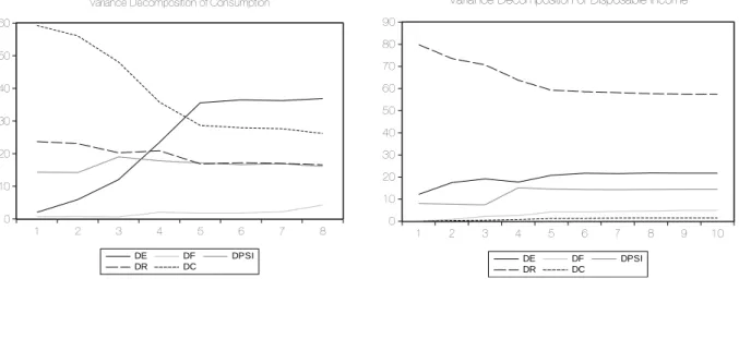
Figure 2 – Variance Decompositions of both Consumption and Disposable Income. Standard deviations not available since we’re using combined graphs.
18
To obtain further information concerning this model, we analyse the variance decomposition of both consumption and disposable income. This way, we can get more insight on the relative importance that each variable’s innovations has in each one of these variables.
From the graphs depicted above, we can verify that consumption is mostly affected by innovations in consumption itself and on energy prices. Energy prices seem to have a longer, more sustained effect and appear to be the more relevant one as time goes by. Innovations in income and stock prices are the 3rd and 4th most relevant forces, according to the variance
decomposition shown in the left-hand graph.
In the case of income, we see that it is dominated by innovations in income itself, with energy coming as the 2nd most relevant variable and stock market coming as 3rd. These results were obtained while following the Cholesky ordering specified above, changes in the order will have an effect on these decompositions. If income and consumption were to change places in the ordering scheme, consumption would become relevant in income’s variance decomposition and income would become less significant in consumption’s decomposition.
Direct and Indirect Effects
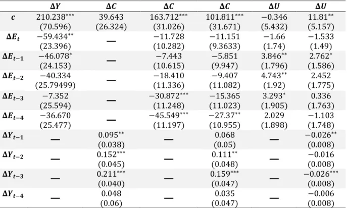
Following the discussion regarding the direct and indirect effects that energy shocks have on consumption, we try to determine which one is more prevalent. Below, we present a table with a summary of the regressions.
Considering the hypothesis that energy prices only have indirect effects, they would become insignificant as we added disposable income as an independent variable. The 1st regression shows how energy price changes are significant in explaining changes in income. If only indirect effects were present in the Portuguese economy, the significant energy related coefficients present in the 3rd regression would be stemming from that indirect relation and reflective of the relation present in the 1st and 2nd equations. Thus, given that the 4th equation
19
features both energy prices and disposable income, significance in the fourth lag of energy price changes suggests either a lagged direct response to price changes or an indirect effect through variables not present in this regression.
𝚫𝒀 𝚫𝑪 𝚫𝑪 𝚫𝑪 𝚫𝑼 𝚫𝑼 𝒄 210.238∗∗∗ (70.596) 39.643 (26.324) 163.712∗∗∗ (31.026) 101.811∗∗∗ (31.671) −0.346 (5.432) 11.81∗∗ (5.157) 𝚫𝑬𝒕 −59.434∗∗ (23.396)
−
−11.728 (10.282) −11.151 (9.3633) −1.66 (1.74) −1.533 (1.49) 𝚫𝑬𝒕−𝟏 −46.078∗ (24.153)−
−7.443 (10.615) −5.851 (9.947) 3.846∗∗ (1.796) 2.762∗ (1.586) 𝚫𝑬𝒕−𝟐 −40.334 (25.79499)−
−18.410 (11.336) −9.407 (11.082) 4.743∗∗ (1.92) 2.452 (1.775) 𝚫𝑬𝒕−𝟑 −7.352 (25.594)−
−30.872∗∗∗ (11.248) −15.365 (11.023) 3.293∗ (1.905) 0.336 (1.763) 𝚫𝑬𝒕−𝟒 −36.670 (25.477)−
−45.549∗∗∗ (11.197) −27.37∗∗ (10.955) 2.029 (1.898) −1.103 (1.748) 𝚫𝒀𝒕−𝟏−
0.095∗∗ (0.038)−
0.068 (0.05)−
−0.026∗∗ (0.008) 𝚫𝒀𝒕−𝟐−
0.152∗∗∗ (0.045)−
0.111∗∗ (0.048)−
−0.016 (0.008) 𝚫𝒀𝒕−𝟑−
0.211∗∗∗ (0.040)−
0.159∗∗∗ (0.047)−
−0.026∗∗∗ (0.008) 𝚫𝒀𝒕−𝟒−
0.048 (0.06)−
0.035 (0.047)−
−0.006 (0.008)Table 1 - Multiple Regressions for Direct and Indirect Effects using OLS. The stars (*,**,***) state statistical significant coefficients at 10%, 5% and 1% significance levels, respectively. Standard deviations for the coefficients are show in parenthesis. The unemployment rate (𝛥𝑈) used in columns 5 and 6 is in percentage points.
The results shown in the 5th and 6th regressions regard unemployment. While some energy related coefficients are significant in the 5th regression, suggesting that energy price movements have an effect in the Portuguese unemployment rate, these become insignificant as we add income in the 6th equation. Hence, this is evidence that energy has only an indirect effect on the unemployment rate. If consumption followed the same pattern regarding energy related coefficients, we could safely vouch for the absence of direct effects.
The equations shown above are somewhat relatable to the Granger Causality, which tests whether or not some time series is relevant in explaining another. The null hypothesis in this test is that variable 𝑥 does not granger cause 𝑧. If we can’t reject it, we should not include
20
contemporaneous and past values of 𝑧 in a regression that attempts to explain 𝑥. We did the tests for income, consumption and energy and got the following results:
Null Hypothesis: Observations F-Statistic P-Value
DE does not Granger Cause DC 77 5.77723 0.0005
DC does not Granger Cause DE 0.30026 0.8768
DR does not Granger Cause DC 77 5.32153 0.0009
DC does not Granger Cause DR 0.83532 0.5075
DR does not Granger Cause DE 77 0.31347 0.8680
DE does not Granger Cause DR 2.12265 0.0874
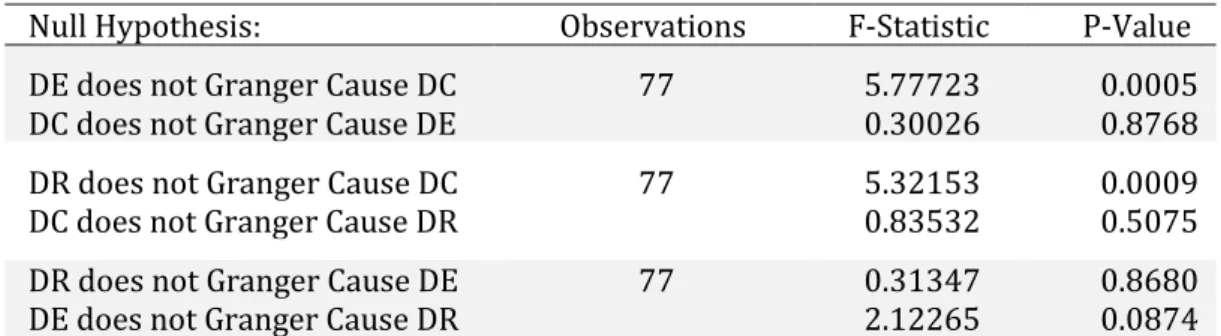
Table 2 – Granger Causality tests for consumption, energy and income. These results are taken from an extended table containing all the variables used in the VAR model.
From the table shown above, we can verify that we have strong statistical evidence that changes in energy prices granger cause changes in consumption and that changes in consumption also do granger cause changes in income. The same evidence is found for energy affecting income but only at 10% significance levels. These results are in accord with the specifications used in the previously mentioned regressions.
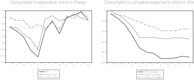
In order to gather more evidence for the presence of the two effects, we isolated the channels through which consumption responds to an energy price shock. To do this, we break the impulse response function using the variables’ coefficients from the VAR model specified above to understand which of them are having the bigger impact. Additionally, we present the cumulative response.
This set of figures shed some light on the responsiveness of consumption, its lag and its origins. The two are slightly different. We are especially interested in the accumulated response function since it will be a better illustration of the total accumulated effects. Both are displayed in the next page.
21
Consumption’s response to shock in Energy Consumption’s cumulative response to shock in Energy
First, it seems to take private consumption half a year to ¾ quarters until its response becomes sizeable. It decreases exponentially until the 5th quarter. By then, the decrease in consumption becomes smoother and stagnates from the 8th quarter on. Thus, both direct and indirect effects take about half a year to become noticeable.
Second of all, we can verify that the direct effect stops roughly on the 5th lag, with the indirect effect fading through until the 8th quarter. Hence, this is evidence that both effects are present in the Portuguese economy3. Furthermore, it also suggests that the direct effect is stronger, although less persistent.
VII. Conclusions
This paper gives use to VAR modeling in order to gain some insight on the economic forces that drive the Portuguese Economy. Specifically, it attempts to understand the power
3 The same analysis was done for the direct and indirect effects of fluctuations in the financial markets.
Although the general behavior is similar, the direct effects are more prevalent in this case and we couldn’t reject the hypothesis that there are no actual indirect effects.
-500 -400 -300 -200 -100 0 1 2 3 4 5 6 7 8 9 10 11 12 IRF Cumulative Direct Cumulative Indirect Cumulative -140 -120 -100 -80 -60 -40 -20 0 20 1 2 3 4 5 6 7 8 9 10 11 12 IRF Direct Effect Indirect Effect
22
and relevance that central markets - with either inelastic demand or supply – have on this particular economy.
It was shown that, apart from food prices, all other variables have relevant and significant effects on private consumption. Fluctuations in both financial markets and energy markets have an impact in the behavior of both income and consumption and, as a result, can potentially lead to a slowdown in economic development.
Thus, the results obtained here show some degree of exposure to unanticipated events that, unfortunately, have been quite common in both the global and the national economies. This can be taken as evidence that, for example, increasing the country’s energy sustainability and energy security can make the economy more stable and immune to foreign shocks.
Additionally, if monopoly power is present in the energy sector, macroeconomic stability and development can be impaired by private decisions. Hence, what the country stands to gain by having a privatized energy sector heavily depends the sector’s structure and balance of power.
Additional interest was taken with respect to the direct and indirect effects of fluctuations in energy prices. As it has been shown, these fluctuations affect consumption both directly – through renewed consumption decisions, arising from shrunken discretionary income and changes in expectations – and indirectly – such as the mechanisms present in Hamilton (1988). The overall effect of energy price movements is estimated to last up to two years.
Relevant further studies on the matters at hand can focus on how to make the Portuguese economy quicker to adapt to such price movements so as to reduce persistence of the negative impacts shown above.
23
VIII. References
Flavin, Marjorie A. 1981. “The Adjustment of Consumption to Changing
Expectations About Future Income.” The Journal of Political Economy, Vol. 89, No. 5, pp. 974-1009
Poterba, James M. and Samwick, Andrew A. 1995. "Stock Ownership Patterns,
Stock Market Fluctuations, and Consumption." Brookings Paper on Economic Activity, 2: 295-372.
Ludvigson, Sydney C. and Steindel, Charles. 1999. “How Important is the stock
Market Effect on Consumption.” Economic Policy Review, Vol. 5, No. 2
Ludwig, Alexander and Slok, Torsten. 2002. “The Impact of Stock Prices and House
Prices on Consumption in OECD Countries.” IMF Working Paper, WP/02/1
Bartaut, Carol C. 2002. “Equity Prices, Household Wealth and Consumption Growth
in Foreign Industrial Countries: Wealth Effects in the 1990’s.” FRB International Finance Discussion Paper No. 724
Groenewold, Nicolaas. 2003. “Consumption and Stock Prices: Can We Distinguish
Signalling from Wealth Effects?” The University of Western Australia, Department of Economics, Economics Discussion / Working Papers, 03-22
de Castro, Gabriela L. 2007. “The Wealth Effect on Consumption in the Portuguese
Economy.” Banco de Portugal, Publications, 37.
Amonhaemanon, Dalina. 2015. “The Impact of Stock Price and Real Estate Price
Shocks on Consumption: The Thai Experience.” International Journal of Financial
Research, Vol 6, No 1
Hamilton, James D. 1998. “A Neoclassical Model of Unemployment and the Business Cycle.” Journal of Political Economy, vol 96, no 3
Dhawan, Rajeev and Jeske, Karsten. 2006. “How Resilient is the Modern Economy
to Energy Price Shocks?” Economic Review, Vol. 91, No. 3.
Hamilton, James D. 2009. “Causes and Consequences of the Oil Shock of 2007-08.”
24
Killian, Lutz. 2007. “The Economic Effects of Energy Price Shocks.” CEPR
Discussion Paper No. DP6559.
van de Ven, D. J., & Fouquet, R. 2014. “Historical energy price shocks and their
changing effects on the economy.” Centre for Climate Change Economics and Policy
Working Paper, (171).
Baghirov, A., & Rodzko, R. 2014. “Direct and indirect effects of oil price shocks
on economic growth: case of Lithuania.” ISM University of Management and Economics.
Campbell, J. Y., & Mankiw, N. G. 1989. “Consumption, income and interest
rates: Reinterpreting the time series evidence.” NBER Macroeconomics Annual 1989,