Equity Valuation of
PUMA SE
Fabian Arndt
Dissertation written under the supervision of
Professor José Carlos Tudela Martins
Dissertation submitted in partial fulfilment of requirements for the MSc in
Finance, at the Universidade Católica Portuguesa, June 6
th2019.
Company: PUMA SE
Industry: Sportswear Listed: Frankfurt Stock Exchange
Bloomberg: PUM GR Reuters: PUMG.DE
Recommendation: HOLD
Target Share Price: €505,91 Current Share Price: €481,50
(as of 13 February 2019) Potential: +5,07% Value Indicators: DCF: 511,99 EV/Sales: €634 | EV/EBITDA: €432 EV/EBIT: €478 | P/E: €485 Investment Summary 80% 100% 120% 140% 160% 180%
Mar-17 Sep-17 Mar-18 Sep-18
3-Year Indexed Weekly Performance
MDAX PUMA
Summary:
The management guidance of Feb 18 for sales growth of 10% was outperformed with 17.6%, ending up in a strong EBIT of €337m. Given a strong global brand recognition momentum across various product lines and a full order book for Q1/19 we expect PUMA to continue its trend on sales growth with 10.4% in FY19 and 10.0% in FY20. We predict the EBIT margin to decrease slightly from 7.3% in FY18 to 7,1% in FY19 and 7.2% in FY20 due to increasing OPEX mainly triggered by a higher level of marketing expenses. CAPEX is expected to increase significantly from €138m in FY18 to €205m in FY19, in line with management guidance (€200m). PUMA transformed its business over the past years by identifying new sport style trends and transforming them into fashionable and high performance products that leverage sales. Furthermore, its marketing strategy to sign high profile celebrities (Rihanna, Selena Gomez, Jay-Z) seems to be paying off well.
World Economy, Industry, Competitors:
The European market is challenging due to Brexit uncertainties and high competition. Opportunities can be seen in the fastest growing region of Asia, where conditions are more favorable.
Despite the strong upwind, PUMA still lacks in market share and brand heat compared to its major competitors Adidas and Nike which results in scale disadvantages when signing sport stars for marketing purpose. Valuation Summary:
The values obtained by the DCF model and multiples are weighted and a price recommendation of €505.91 is issued. Compared to the share price of €481.50 it demonstrates a 12-month upside potential of 5.07%. Overall, this leads to a HOLD recommendation for PUMA shares. Valuation Notes:
Two different valuation approaches were applied to receive a fair value share price of PUMA. On the one hand, the DCF valuation yields a price of €511.99, representing an upside potential of 6.33%. On the other hand, the 1-year forward multiple approach including EV/Sales, EV/EBITDA, EV/EBIT and P/E result in a median indicated price of €633.10, €431.71, €477.28 and €484.86, respectively.
14 February 2019
Column1 1W 1M 3M
Absolute 0.21% 4.79% 6.88%
Relative (vs. MDAX) -0.03% -0.86% 7.66%
Current Share Price 481.50 €
52-Week High 525.00 € 52-Week Low 317.00 € Column1 Column2 2018 2019 DCF WACC 5.85% Tax Rate 26.57%
Revenue CAGR FY19-FY27 7.48%
Terminal Growth Rate 2.20%
Multiples EV/Sales 1.9x EV/EBITDA 14.7x EV/EBIT 20.2x P/E 30.8x Column1 2016 2017 2018 Gross Margin 45.7% 47.3% 48.4% EBITDA Margin 5.2% 7.6% 9.0% EBIT Margin 3.5% 5.9% 7.3% Pretax ROE 7.2% 13.9% 18.8% Current Ratio 1.05 1.78 1.83 x Interest Earned 9.50 13.70 22.40
Cash Cycle (Days) 76 67 75
D / E Ratio 2.4% 3.7% 11.8%
Net Debt / Equity -16.7% -21.8% -15.4%
Stock Performance
Valuation Metrics
Key Ratios (Historical) 05 June 2018 14 February 2018 13 February 2019
in €m 2014 2015 2016 2017 2018 2019E 2020E 2021E 2022E 2023E 2024E 2025E 2026E 2027E TV
Revenues 2,972 3,387 3,627 4,136 4,648 5,131 5,644 6,187 6,842 7,453 7,992 8,416 8,703 8,894 9,090
Change Sales Y-o-Y -0.4% 14.0% 7.1% 14.0% 12.4% 10.4% 10.0% 9.6% 10.6% 8.9% 7.2% 5.3% 3.4% 2.2% 2.2%
EBIT 128 96 128 245 337 363 409 453 492 520 532 559 578 590 603 EBIT Margin 4.3% 2.8% 3.5% 5.9% 7.3% 7.1% 7.2% 7.3% 7.2% 7.0% 6.7% 6.6% 6.6% 6.6% 6.6% EBITDA 186 154 188 315 419 454 507 559 609 647 669 704 727 743 759 EBITDA Margin 6.3% 4.5% 5.2% 7.6% 9.0% 8.8% 9.0% 9.0% 8.9% 8.7% 8.4% 8.4% 8.4% 8.4% 8.3% Net Income 64 37 62 136 187 235 264 293 319 337 347 367 380 391 401 NOPAT 254 266 300 332 361 382 391 411 424 433 443 FCFF 87 32 104 124 121 158 192 256 319 363 407 # Shares Outstanding 14.95 14.95 14.95 14.95 14.95 14.95 14.95 14.95 14.95 14.95 14.95 14.95 14.95 14.95 14.95 EPS (€) 4.29 2.48 4.18 9.08 12.53 15.73 17.69 19.58 21.31 22.58 23.25 24.52 25.45 26.14 26.84 Dividend per Share (€) 0.50 0.50 0.75 12.50 3.50 3.93 4.42 4.90 5.33 5.64 5.81 6.13 6.36 6.53 6.71 Cash & Cash Equivalents 402 339 327 415 464 385 408 443 467 523 612 761 972 1226 1487 Net Debt -381 -318 -285 -355 -263 -165 -167 -179 -178 -207 -268 -388 -569 -792 -1021
List of Contents
List of Contents ... I List of Figures ... IV List of Tables ... VI List of Abbreviations ... VII List of Formulas ... X Abstract ... 1 Resumo ... 1 Acknowledgement ... 2 1 Introduction ... 3 2 Literature Review ... 4
2.1 Fundamentals of Intrinsic Valuation Methods ... 4
2.1.1 Discount Rate ... 4
2.1.2 Cost of Equity ... 5
2.1.2.1 Risk-free Rate ... 6
2.1.2.2 Beta ... 6
2.1.2.3 Market Risk Premium ... 7
2.1.3 Cost of Debt ... 7
2.1.4 Weighted Average Cost of Capital ... 8
2.2 Valuation Approaches ... 8
2.2.1 Dividend Discount Model ... 9
2.2.2 Discounted Free Cash Flow Model ... 10
2.2.2.1 Free Cash Flow to the Firm ... 10
2.2.2.2 Free Cash Flow to Equity ... 11
II
2.2.4 Terminal Growth Rate and Terminal Value ... 13
2.2.5 Option Pricing Model (Real Options) ... 14
2.2.6 Asset-based valuation ... 14
2.2.7 Multiples / Relative Approach ... 14
3 Global Economy Overview ... 16
4 Industry Overview ... 19
5 Company Overview ... 24
6 DCF Valuation ... 35
6.1 Financial Forecast - Income Statement ... 35
6.2 Financial Forecast – Balance Sheet ... 46
6.3 Discount Rate ... 50
6.3.1 Cost of Debt ... 50
6.3.2 Cost of Equity ... 51
6.3.2.1 Risk Free Rate ... 51
6.3.2.2 Beta ... 52
6.3.2.3 Market Risk Premium ... 52
6.3.3 WACC Calculation ... 53
6.4 Long-term Growth Rate ... 53
6.5 Discounted Cash Flow ... 54
6.6 Sensitivity Analysis ... 56
7 Multiples / Relative Valuation ... 57
7.1 Peer Group Selection ... 57
7.2 Relative Valuation ... 58
8 Sum of the parts valuation ... 60
9 Comparison Investment Bank Report ... 61
III 11 Appendix ... 64 12 Publication bibliography ... 74
IV
List of Figures
Figure 1: Real GDP growth 2008 - 2024E ... 16
Figure 2: Inflation rates 2008 - 2024E ... 17
Figure 3: 10-Year sovereign bond yield average ... 17
Figure 4: Short-term interest rates 2008 - 2020E ... 18
Figure 5: Long-term interest rates 2008 - 2020E ... 18
Figure 6: Market Share of the largest sportswear producers ... 19
Figure 7: Market size and segment overview ... 21
Figure 9: Market growth by region ... 22
Figure 8: Global sportswear market ... 22
Figure 10: Revenue split by segment ... 24
Figure 11: Sales across segments ... 24
Figure 12: EMEA sales & growth Figure 13: Americas sales & growth ... 25
Figure 14: APAC sales & growth ... 25
Figure 15: Distribution channel mix ... 26
Figure 16: Sourcing regions of PUMA in % of unit production in FY18. ... 26
Figure 17: Sponsorships (a) ... 27
Figure 18: Sponsorships (b) ... 28
Figure 19: Sustainability goals ... 28
Figure 20: Social media followers ... 29
Figure 21: Sales and EBIT margin ... 30
Figure 22: EBIT vs. EBIT/FTE ... 31
Figure 23: Sales vs. Sales/FTE ... 31
V Figure 25: PUMA SE 5-year share price development compared to the MDAX index 33 Figure 26: PUMA SE 3-year share price development compared to the MDAX index 33
Figure 27: Dividend per share ... 34
Figure 28: Ownership structure ... 34
Figure 29: Revenue growth forecast ... 35
Figure 30: Sales development and growth rates ... 37
Figure 31: Cost structure in relation to sales ... 39
Figure 32: EBIT and EBIT margin ... 40
Figure 33: Financial expenses ... 41
Figure 34: Net income and net income margin ... 42
Figure 35: Net income bridge FY18 ... 43
Figure 36: PP&E + Intangibles and D&A ratio ... 44
Figure 37: CAPEX development and forecast ... 44
Figure 38: CAPEX and D&A ... 45
Figure 39: Net debt ... 46
Figure 40: Cash conversion cycle ... 48
Figure 41:After-tax cost of debt ... 50
Figure 42: 10-Year sovereign bond yields ... 51
Figure 43: Beta regression MSCI World Figure 44: Beta regression MDAX ... 52
Figure 45: Summary WACC Calculation ... 53
VI
List of Tables
Table 1: Overview of frequently used multiples ... 15
Table 2: Market share development among the 10 largest sportswear producers ... 20
Table 3: Key financial figures ... 30
Table 4: Revenue forecast summary ... 36
Table 5: Capital structure ... 47
Table 6: Change Net Working Capital ... 49
Table 7: Terminal growth rate ... 54
Table 8: DCF - Free Cash Flow to the Firm ... 55
Table 9: Sensitivity analysis - Equity Value ... 56
Table 10: Sensitivity analysis - Share Price ... 56
Table 11: Peer company selection criteria ... 57
Table 12: Peer companies ... 57
Table 13: Relative valuation summary ... 59
Table 14: Share Price Summary ... 60
VII
List of Abbreviations
$ ... Dollar (Currency) % ... Percentage & ... And € ... Euro (Currency) AG ... Aktiengesellschaft APV ... Adjusted Present Value Bn ... BillionCAGR ... Compound Annual Growth Rate CAPEX ... Capital Expenditures
CAPM ... Capital Asset Pricing Model CCC ... Cash Conversion Cycle CEO ... Chief Executive Officer CF ... Cash Flow
COGS ... Cost of Goods Sold Corp ... Corporation
DAX ... Deutscher Aktienindex DCF ... Discounted Cash Flow DDM ... Dividend Discount Model DIO ... Days Inventory Outstanding DPO ... Days Payable Outstanding DSO ... Days Sales Outstanding DPS ... Dividend per Share
E.g. ... exempli gratia (for example) EPS ... Earnings per Share
FCF ... Free Cash Flow E ... Equity
EBIT ... Earnings before Interest and Taxes
EBITDA ... Earnings before Interest Taxes Depreciation & Amortization ECB ... European Central Bank
VIII FCFE ... Free Cash Flow to Equity
FCFF ... Free Cash Flow to the Firm
FIFA ... Fédération Internationale de Football Association FX ... Foreign Exchange
FX ... Foreign Exchange FY ... Financial Year
GDP ... Gross Domestic Product GGM ... Gordon Growth Model H ... Half (year)
IAS ... International Accounting Standards IDW ... Institut Deutscher Wirtschaftspruefer
IFRS ... International Financial Reporting Standards IMF ... International Monetary Fund
Inc. ... Incorporation K ... Thousand
KPMG ... Klynveld Peat Marwick Goerdeler (Accounting Firm) M ... Million
MDAX ... Midcap-DAX
MRP ... Market Risk Premium
MSCI World ... Morgan Stanley Capital International World NOPAT ... Net operating profit after tax
OECD ... Organization for Economic Co-operation and Development P ... Price
PER ... Price to Earnings Ratio ROE ... Return on Equity
ROIC ... Return on Invested Capital TV ... Terminal Value
PP&E ... Property, Plant & Equipment R&D ... Research & Development SE ... Societas Europeae
SG&A ... Selling, General and Administrative Expense US ... United States
IX WACC ... Weighted Average Cost of Capital
WC ... Working Capital Y ... Year
Y-o-Y ... Year-over-Year YTM ... Yield-to-Maturity
X
List of Formulas
Formula 1: Discounted cash flow model ... 4
Formula 2: Cost of equity ... 5
Formula 3: Unlevered beta ... 6
Formula 4: Levered Beta ... 7
Formula 5: Blume adjustment ... 7
Formula 6: Weighted average cost of capital ... 8
Formula 7: Dividend discount model ... 9
Formula 8: Gordon growth model ... 9
Formula 9: Two-stage dividend discount model ... 9
Formula 10: Free Cash Flow to the Firm ... 10
Formula 11: Discounted free cash flow to the firm ... 10
Formula 12: Free cash flow to equity ... 11
Formula 13: Discounted FCFE ... 11
Formula 14: Adjusted present value ... 12
Formula 15: Value of tax benefits ... 12
Formula 16: APV - Sum of parts ... 12
Formula 17: Terminal value ... 13
1
Abstract
The purpose of the dissertation is to determine a target price per share for the sportswear pro-ducer PUMA SE that is listed on the German MDAX. Based on this value and relative to the current market price, a buy, hold or sell recommendation is provided. Hence, the underlying research question of this dissertation is: “What is the fair value per share for PUMA SE on 31
December 2018 and the implied investment recommendation on 13 February 2019?”. The
ob-tained share price is based on a combination of two valuation methods: The discounted cash flow model and a relative valuation approach based on multiples that result in a price per share of €505.91. The valuation is an outcome of a comprehensive market, industry and company analysis. By comparing the computed share price with the current market price of €481.50 as of 13 February 2019, a hold recommendation with upside potential of 5.07% is issued. Finally, selected assumptions and results are compared with the equity report of PUMA SE from War-burg Research. All information and data in this publication stem from publicly available sources.
Author: Fabian Arndt
Title: Equity Valuation of PUMA SE
Key words: Equity Valuation, Corporate Finance, Share Price, DCF, Multiples, PUMA SE
Resumo
A dissertação tem como propósito determinar o preço intrínseco por ação da marca desportiva PUMA SE, cotada na bolsa alemã MDAX. Com base nesta avaliação é recomendada uma es-tratégia de compra, venda ou neutral face ao preço de mercado atual. Deste modo, esta dis-sertação pretende responder à seguinte pergunta: “Qual era o valor intrínseco por ação da
PUMA SA a 31 de dezembro de 2018 e qual a estratégia de investimento recomendada a 13 de fevereiro de 2019?” Tendo em conta a análise do mercado e da indústria em que a PUMA SE
se insere, o valor intrínseco por ação da empresa é de €505.91 Esta avaliação baseou-se essen-cialmente em dois métodos de avaliação: cash flows descontados e múltiplos prospetivos, util-zando múltiplos de mercado. Comparando o valor intrínseco da empresa com o preço de mer-cado registado a 13 de fevereiro de 2019, recomenda-se uma estratégia de neutral, com um ganho potencial de 5,07% caso o preço de mercado iguale o valor intrínseco da empresa. Por último, toda a informação necessária para esta análsie foi recolhida em fontes públicas e todos os resultados e assunções presentes foram comparados com o previsão sobre Puma SE do War-burg Research”.
Autor: Fabian Arndt
Título: Equity Valuation of PUMA SE
2
Acknowledgement
The steps towards my master dissertation were the most formative of my lifetime. It was an eventful path that made me grow personally and academically. All my achievements and expe-riences wouldn’t be possible without the support of my personal surroundings for what reason I want to share my sincere appreciation, at least with a few words.
A special thanks goes to my parents and my sister who always believed in me and gave support beyond my needs.
Moreover, I want to thank my childhood friends, Michael and Richard, Jonas and many others; even though I wasn’t there for a long time, our friendship never weakened.
During my masters at Católica, my colleagues became friends who always brought me joy dur-ing this intense program. Thank you, Peter, Roman, Tom and all the others that brought life at Católica and outside the classroom not just one level up. Thank you, Gregor and Nicolas, for making my exchange semester in Rio de Janeiro an unforgettable adventure. Thank you, Marta, for this wonderful experience during my stay in Lisbon. Thank you, Martin and Denis, for our insightful discussions and your great support for my thesis.
Finally, I would like to thank Professor Tudela Martins for the excellent support and guidance for this dissertation.
3
1 Introduction
The valuation of a company serves to determine the theoretical price for a company. The value of a company may differ for buyers, sellers or other parties (Fernández 2002).
The objective of this dissertation is to provide a rational and reliable valuation of PUMA SE, a sportswear producer and distributer, publicly listed on the German MDAX. The fair value share price is estimated based on the company´s results as of 31 December 2018 and subsequently compared with the market price on 13 February 2019, the day before the publication of PUMA’s annual report for fiscal year 2018. This comparison of prices enables potential investors an adequate basis for a buy, hold or sell decision. Thus, the research question for this dissertation is formulated as follows:
What is the fair value per share for PUMA SE on 31 December 2018 and the implied investment recommendation on 13 February 2019?
This evaluation is based on publicly available information from PUMA as well as other public market information. The paper is organized as follows: The second section provides an over-view of general company valuation literature and is contextualized by means of PUMA's char-acteristics. The third section gives an overview of the current situation of the world economy in the context of PUMA´s exposure. In section four, the sports apparel industry is analyzed to discover opportunities and risks in this sector and to identify relevant forecast indicators. The fifth section is a detailed company analysis based on financial, operational and strategic factors. The DCF valuation is explained in chapter six, followed by an illustration of the relative valu-ation in chapter seven. Chapter eight summarizes the results of the conducted valuvalu-ation ap-proaches, including a buy, hold or sell recommendation. In chapter nine, the obtained results are compared with an equity research report of PUMA by Warburg Research. Chapter 10 con-cludes all valuation results.
4
2 Literature Review
The term value is endowed with a variety of definitions, but for the purpose of this work it is the result of calculating the equity of a firm, or shareholder value, which is the part of a company that belongs to its shareholders. This value can be obtained by three distinct methods: First, the intrinsic valuation methods which are based on future cash flow projections. Second, the real options approach, where option pricing techniques help to determine the value of the company. Third, the relative valuation methods that use similar companies with a known market value to estimate the value of the underlying company’s shares (Pereiro 2002).
The most prevailing methods for analysts to estimate the value of a company are discounted cash flow models and relative approaches according to Demirakos et al. (2004). Other methods are the asset-based valuation and the real option valuation. The following valuation models are selected based on the characteristics of PUMA SE.
2.1 Fundamentals of Intrinsic Valuation Methods
Intrinsic valuation models measure the value of a company based on the present value of its projected cash flows at a risk-adjusted discount rate (Reilly and Brown 2011). Specific com-pany characteristics are the crucial components in order to identify the intrinsic values of its assets. A general formula for estimating the value of a firm by discounting expected cash flows can be described as follows (Rosenbaum and Pearl 2009).
𝑉𝑖 = ∑ 𝐶𝐹𝑡 (1 + 𝑘)𝑡 𝑛 𝑡=1 (1) Where: 𝑉𝑗= 𝑉𝑎𝑙𝑢𝑒 𝑜𝑓 𝑠𝑡𝑜𝑐𝑘 𝑖 𝐶𝐹𝑡= 𝐶𝑎𝑠ℎ 𝑓𝑙𝑜𝑤 𝑎𝑡 𝑝𝑒𝑟𝑖𝑜𝑑 𝑡 𝑘 = 𝐷𝑖𝑠𝑐𝑜𝑢𝑛𝑡 𝑟𝑎𝑡𝑒 𝑛 = 𝐶𝑜𝑢𝑛𝑡 𝑜𝑓 𝑦𝑒𝑎𝑟𝑠 𝑜𝑓 𝑡ℎ𝑒 𝑙𝑖𝑓𝑒𝑡𝑖𝑚𝑒 𝑜𝑓 𝑎𝑠𝑠𝑒𝑡 𝑖
Formula 1: Discounted cash flow model
To understand the concepts of discounting cash flow models, it is essential to master the funda-mentals of discount rates. For that reason, the principles of this methodology are explained in the following chapters.
2.1.1 Discount Rate
The discount rate determines the present value of future cash flows and is a function of the riskiness of forecast cash flows (Damodaran 2012). Depending on the valuation approach, the
5 discount factor consists of the components cost of equity or a combination of cost of equity and cost of debt.
2.1.2 Cost of Equity
The cost of equity can be estimated using the capital asset pricing model (CAPM), based on the portfolio theory of Markowitz (1952) and is independently developed by Sharpe (1964), Lintner (1965) and Mossin (1966). Until today it is the most widely used model in valuation practice to determine the expected return of an investment. The CAPM is based on a one-period model with equilibrium in the capital markets under specific assumptions.1 The fundamental equation
of the CAPM describes the relationship between the expected return of an investment on the capital market and its risk (Ross 1977).
𝐸(𝑅𝑖) = 𝑟𝑓+ (𝐸(𝑅𝑚) − 𝑟𝑓) × 𝛽𝑖 (2) Where: 𝐸(𝑅𝑖) = 𝐸𝑥𝑝𝑒𝑐𝑡𝑒𝑑 𝑟𝑒𝑡𝑢𝑟𝑛 𝑜𝑓 𝑖𝑛𝑣𝑒𝑠𝑡𝑚𝑒𝑛𝑡 𝑖 𝑟𝑓 = 𝑅𝑖𝑠𝑘-𝑓𝑟𝑒𝑒 𝑟𝑎𝑡𝑒 𝐸(𝑅𝑚) = 𝐸𝑥𝑝𝑒𝑐𝑡𝑒𝑑 𝑟𝑒𝑡𝑢𝑟𝑛 𝑜𝑓 𝑡ℎ𝑒 𝑚𝑎𝑟𝑘𝑒𝑡 𝛽𝑖= 𝐵𝑒𝑡𝑎 (𝑠𝑦𝑠𝑡𝑒𝑚𝑎𝑡𝑖𝑐 𝑟𝑖𝑠𝑘)
Formula 2: Cost of equity
The core thesis states that in a capital market equilibrium, the expected return of any risky investment 𝐸(𝑅𝑖) equals a risk-free return 𝑟𝑓 plus a risk premium. This risk premium results from the multiplication of the market risk premium (MRP) with the systematic risk 𝛽𝑖. The MRP measures to the price that investors demand for the risk of the investment and is described by (𝐸(𝑅𝑚) − 𝑟𝑓) (Koller et al. 2015). The expected return is equivalent to the cost of equity. It is explained as the required return by investors to invest in this company rather than in an alter-native investment. In other words, the cost of equity corresponds to opportunity costs for the equity holder (Frykman and Tolleryd 2003). Alternatively to the CAPM, the Fama and French 3-Factor model proposed by Fama, E. F./French, K. R. (1993) can be applied. Due to its prac-ticability, the CAPM is preferred by analysts and is consequently applied for the valuation of PUMA.
6
2.1.2.1 Risk-free Rate
The risk-free rate corresponds to an investment with riskless characteristics (Koller et al. 2015). The investment is risk-free if there is no deviation from its expected return, so that the actual return is equal to the expected return. According to the literature, sovereign bonds are preferred to replicate this riskless investment. Damodaran (2008) and other authors suggest a 10-year AAA-rated government bond to comply with the period of the forecasted cash flows of the company. Beyond that, the bond must be traded and denominated in the same currency in which the company operates (Koller et al. 2015; Damodaran 2008).
2.1.2.2 Beta
The beta factor measures the systematic risk that cannot be eliminated by diversifying a portfo-lio of securities. The unsystematic risk reflects the investment-specific risk, for example due to management errors or credit risk. This risk can be remedied by diversifying the portfolio (Copeland et al. 2007).
Common sources like Bloomberg or Reuters provide beta estimations but are often imprecise. It is suggested to use a set of peer group betas from the same industry on a levered basis and modify it for a firms’ financial leverage to obtain the unlevered beta (Koller et al. 2015).
𝛽𝑢 = 𝛽𝑙 1 + (1 − 𝑡) ∗ (𝐷𝐸) (3) Where: 𝛽𝑢= 𝑈𝑛𝑙𝑒𝑣𝑒𝑟𝑒𝑑 𝑏𝑒𝑡𝑎 𝛽𝑙= 𝐿𝑒𝑣𝑒𝑟𝑒𝑑 𝑏𝑒𝑡𝑎 𝑡 = 𝐶𝑜𝑟𝑝𝑜𝑟𝑎𝑡𝑒 𝑡𝑎𝑥 𝑟𝑎𝑡𝑒 𝐷 = 𝐷𝑒𝑏𝑡 𝐸 = 𝐸𝑞𝑢𝑖𝑡𝑦
Formula 3: Unlevered beta
Another method is a regression by dividing the covariance of the historical returns of the in-vestment 𝑖 and the return of the market portfolio m divided by the variance of the market port-folio’s returns. The market portfolio can be a national market index or an international index such as the MSCI World Index (Koller et al. 2015).
7 𝛽𝑖 = 𝜎(𝑅𝑖, 𝑅𝑚) 𝜎𝑚2 (4) Where: 𝛽𝑖= 𝐵𝑒𝑡𝑎 𝑜𝑓 𝑖𝑛𝑣𝑒𝑠𝑡𝑚𝑒𝑛𝑡 𝑖 𝜎(𝑅𝑖, 𝑅𝑚) = 𝐶𝑜𝑣𝑎𝑟𝑖𝑎𝑛𝑐𝑒 𝑜𝑓 𝑖𝑛𝑣𝑒𝑠𝑡𝑚𝑒𝑛𝑡 𝑖 𝑢𝑛𝑑 𝑚𝑎𝑟𝑘𝑒𝑡 𝑝𝑜𝑟𝑡𝑓𝑜𝑙𝑖𝑜 𝑚 𝜎𝑚2 = 𝑉𝑎𝑟𝑖𝑎𝑛𝑐𝑒 𝑜𝑓 𝑡ℎ𝑒 𝑚𝑎𝑟𝑘𝑒𝑡 𝑝𝑜𝑟𝑡𝑓𝑜𝑙𝑖𝑜 𝑚
Formula 4: Levered Beta
There is evidence that by using regressions the forecasted betas are closer to one than the de-termined values calculated from historical data. For this reason, Blume (1979) suggests the fol-lowing adjustment which is also applied for the DCF valuation of PUMA.
𝐴𝑑𝑗𝑢𝑠𝑡𝑒𝑑 𝛽𝑖 = 2 3∗ 𝑟𝑎𝑤 𝛽𝑖 + 1 3∗ 𝑟𝑎𝑤 𝛽𝑚 (5) Where: 𝛽𝑖= 𝐵𝑒𝑡𝑎 𝑜𝑓 𝑖𝑛𝑣𝑒𝑠𝑡𝑚𝑒𝑛𝑡 𝑖 𝛽𝑚= 𝐵𝑒𝑡𝑎 𝑜𝑓 𝑡ℎ𝑒 𝑚𝑎𝑟𝑘𝑒𝑡 𝑝𝑜𝑟𝑡𝑓𝑜𝑙𝑖𝑜 = 1
Formula 5: Blume adjustment
2.1.2.3 Market Risk Premium
The market risk premium (MRP) is defined as the difference between the expected return of the market portfolio and the risk-free return. The MRP corresponds to the additional return required for investments in a diversified portfolio of risky assets above the risk-free interest rate. There are various models for assessing the MRP (Damodaran 2006). However, the adequate value is highly discussed among academics. Koller et al. (2015) proposes a MRP of approximately 5%, Frykman and Tolleryd (2003) suggest a rate between 5% and 6% and KPMG in its recommen-dation of 7% in its latest quarterly issued publication (KPMG 2018a). In Germany, the Institute of Public Auditors in Germany (IDW) recommends a range between 5.5%-7%. A value within this range is used for assessing the CAPM for PUMA.
2.1.3 Cost of Debt
The cost of debt describes the funding costs of a company’s borrowings. If the entity has fre-quently traded debt, the calculation is relatively simple. In this case, the after-tax yield to ma-turity (YTM) on the long-term debt is used as a proxy. The after-tax YTMs include the tax shield in the WACC. Scholars argue that the low default probability of these companies makes possible noise negligible (Koller et al. 2015). Without bonds, reliable independent credit ratings provide comparable values from peer companies with outstanding bonds. If there is no rating
8 assigned, the creation of synthetic ratings canhelp with an approximation (Damodaran 2012). As PUMA has negative net debt in its target capital structure, the calculation of the cost of debt is negligible for the discount rate that is described in the following chapter.
2.1.4 Weighted Average Cost of Capital
The weighted average cost of capital (WACC) is the discount rate that represents the weighted average costs of a company’s equity and debt. It reflects the risk of the projected free cash flows. The cost of debt is reduced by the corresponding tax rate to reflect the arising interest tax shields (Damodaran 2011). 𝑊𝐴𝐶𝐶 = 𝑘𝑑 ∗ (1 − 𝑡) ∗ 𝐷 𝐷 + 𝐸+ 𝑘𝑒 ∗ 𝐸 𝐷 + 𝐸 (6) Where: 𝑊𝐴𝐶𝐶 = 𝑊𝑒𝑖𝑔ℎ𝑡𝑒𝑑 𝑎𝑣𝑒𝑟𝑎𝑔𝑒 𝑐𝑜𝑠𝑡 𝑜𝑓 𝑐𝑎𝑝𝑖𝑡𝑎𝑙 𝐷 = 𝑀𝑎𝑟𝑘𝑒𝑡 𝑣𝑎𝑙𝑢𝑒 𝑜𝑓 𝑑𝑒𝑏𝑡 𝐸 = 𝑀𝑎𝑟𝑘𝑒𝑡 𝑣𝑎𝑙𝑢𝑒 𝑜𝑓 𝑒𝑞𝑢𝑖𝑡𝑦 𝑘𝑑= 𝐶𝑜𝑠𝑡 𝑜𝑓 𝑑𝑒𝑏𝑡 = 𝑟𝑒𝑞𝑢𝑖𝑟𝑒𝑑 𝑟𝑎𝑡𝑒 𝑜𝑓 𝑟𝑒𝑡𝑢𝑟𝑛 𝑏𝑦 𝑑𝑒𝑏𝑡 ℎ𝑜𝑙𝑑𝑒𝑟𝑠 𝑘𝑒= 𝐶𝑜𝑠𝑡 𝑜𝑓 𝑒𝑞𝑢𝑖𝑡𝑦 = 𝑟𝑒𝑞𝑢𝑖𝑟𝑒𝑑 𝑟𝑎𝑡𝑒 𝑜𝑓 𝑟𝑒𝑡𝑢𝑟𝑛 𝑏𝑦 𝑒𝑞𝑢𝑖𝑡𝑦 ℎ𝑜𝑙𝑑𝑒𝑟𝑠 𝑡 = 𝑇𝑎𝑥 𝑟𝑎𝑡𝑒
Formula 6: Weighted average cost of capital
Higher discount rates imply riskier cash flows. The riskiness is defined as the likelihood of default as well as the variation of the actual returns around the expected returns (Damodaran 2011). An important prerequisite for an appropriate use of the WACC is to define a target debt ratio or a constant leverage ratio (Fernandez 2006; Booth 2002).
There is a wide discussion about a suitable tax rate. Damodaran (2012) prefers the effective tax rate for early forecasts and the marginal tax rate in perpetuity. He argues that it is dangerous to assume that taxes can be deferred forever. Other authors argue to apply the effective tax rate. Fernandez (2006) relies on the application of the effective tax rate for international operating companies due to taxation differences in each country. On this basis, PUMA’s valuation model is based on the average effective tax rate of the last three years.
2.2 Valuation Approaches
There exist several discounted cash flow methods that can be applied to determine the value of the asset. In the following, three widely used models are evaluated.
9
2.2.1 Dividend Discount Model
The dividend discount model (DDM) is the longest existing present value model. By applying this approach, dividends represent an appropriate definition of future cash flows (Pinto et al. 2015). Hereinafter, the value of an ordinary stock is hereinafter the present value of future div-idends (Reilly and Brown 2011; Williams 1938).
𝑉0 = ∑ 𝐷𝑡 (1 + 𝑘𝑒)𝑡 𝑛 𝑡=1 (7) Where: 𝑉0= 𝑆𝑡𝑜𝑐𝑘 𝑣𝑎𝑙𝑢𝑒 𝑎𝑡 𝑡𝑖𝑚𝑒 0 𝐷𝑡= 𝐸𝑥𝑝𝑒𝑐𝑡𝑒𝑑 𝑑𝑖𝑣𝑖𝑑𝑒𝑛𝑑 𝑝𝑒𝑟 𝑠ℎ𝑎𝑟𝑒 𝑖𝑛 𝑦𝑒𝑎𝑟 𝑡 (𝑒𝑛𝑑 𝑜𝑓 𝑦𝑒𝑎𝑟 𝑝𝑎𝑦-𝑜𝑢𝑡) 𝑘𝑒= 𝐷𝑖𝑠𝑐𝑜𝑢𝑛𝑡 𝑟𝑎𝑡𝑒 𝑎𝑡 𝑡ℎ𝑒 𝑟𝑒𝑞𝑢𝑖𝑟𝑒𝑑 𝑟𝑎𝑡𝑒 𝑜𝑓 𝑟𝑒𝑡𝑢𝑟𝑛 𝑜𝑛 𝑒𝑞𝑢𝑖𝑡𝑦
Formula 7: Dividend discount model
The implied problems arise with the impossibility of an infinite dividend forecast. A simplifi-cation such as the Gordon Growth Model (GGM), which assumes constant growth rates for the dividends in an indefinite time horizon must be applied (Gordon and Shapiro 1956).
𝑉0 =𝐷𝑡−1∗ (1 + 𝑔) 𝑘𝑒− 𝑔 𝑜𝑟 𝑉0 = 𝐷𝑡 𝑘𝑒− 𝑔 (8) Where: 𝑉0= 𝑆𝑡𝑜𝑐𝑘 𝑣𝑎𝑙𝑢𝑒 𝑎𝑡 𝑡𝑖𝑚𝑒 0 𝐷𝑡= 𝐸𝑥𝑝𝑒𝑐𝑡𝑒𝑑 𝑑𝑖𝑣𝑖𝑑𝑒𝑛𝑑 𝑝𝑒𝑟 𝑠ℎ𝑎𝑟𝑒 𝑎𝑡 𝑡𝑖𝑚𝑒 𝑡 (𝑒𝑛𝑑 𝑜𝑓 𝑦𝑒𝑎𝑟 𝑝𝑎𝑦-𝑜𝑢𝑡) 𝑘𝑒= 𝐷𝑖𝑠𝑐𝑜𝑢𝑛𝑡 𝑟𝑎𝑡𝑒 𝑎𝑡 𝑡ℎ𝑒 𝑟𝑒𝑞𝑢𝑖𝑟𝑒𝑑 𝑟𝑎𝑡𝑒 𝑜𝑓 𝑟𝑒𝑡𝑢𝑟𝑛 𝑜𝑛 𝑒𝑞𝑢𝑖𝑡𝑦 𝑔 = 𝐸𝑥𝑝𝑒𝑐𝑡𝑒𝑑 𝑐𝑜𝑛𝑠𝑡𝑎𝑛𝑡 𝑔𝑟𝑜𝑤𝑡ℎ 𝑟𝑎𝑡𝑒
Formula 8: Gordon growth model
If the growth rate is expected to be higher than the cost of equity, a two-stage DDM for an n-period investment horizon should be applied (Pinto et al. 2015).
𝑉0 = ∑ 𝐷𝑡 (1 + 𝑘𝑒)𝑡 + 𝑉𝑛 (1 + 𝑘𝑒)𝑛 ∞ 𝑡=1 (9) Where: 𝑉0= 𝑆𝑡𝑜𝑐𝑘 𝑣𝑎𝑙𝑢𝑒 𝑎𝑡 𝑡𝑖𝑚𝑒 0 𝐷𝑡= 𝐸𝑥𝑝𝑒𝑐𝑡𝑒𝑑 𝑑𝑖𝑣𝑖𝑑𝑒𝑛𝑑 𝑝𝑒𝑟 𝑠ℎ𝑎𝑟𝑒 𝑖𝑛 𝑦𝑒𝑎𝑟 𝑡 (𝑒𝑛𝑑 𝑜𝑓 𝑦𝑒𝑎𝑟 𝑝𝑎𝑦-𝑜𝑢𝑡)
𝑘𝑒= 𝐷𝑖𝑠𝑐𝑜𝑢𝑛𝑡 𝑟𝑎𝑡𝑒 at the required rate of return on equity
𝑉𝑛= 𝑇𝑒𝑟𝑚𝑖𝑛𝑎𝑙 𝑝𝑟𝑖𝑐𝑒 𝑝𝑒𝑟 𝑠ℎ𝑎𝑟𝑒 𝑖𝑛 𝑝𝑒𝑟𝑖𝑜𝑑 𝑛
10
2.2.2 Discounted Free Cash Flow Model
The DCF Model is the most popular approach among practitioners to estimate the firm value (Mukherjee et al. 2005). Two variations are defined in the following chapters.
2.2.2.1 Free Cash Flow to the Firm
The free cash flow to the firm (FCFF) is the available cash flow to the company’s suppliers of capital after paying all operating expenses (including taxes), as well as investing in all necessary working and fixed capital (Pinto et al. 2015). It can be directly derived by summing the follow-ing items to the net income.
Earnings before interest and tax (EBIT) (10)
(-) Tax on EBIT
= Net operating profit after taxes (NOPAT) (+) Depreciation
(+) Provisions
(+) Other non-cash charges
(-) Investments in net working capital (-) Capital expenditures
= Free cash flow from operations
(+/-) Cash flow from non-operating activities = Free cash flow to the firm (FCFF)
Formula 10: Free Cash Flow to the Firm
The value of the firm can be calculated by discounting the free cash flows with the WACC (Pinto et al. 2015). 𝐸𝑛𝑡𝑒𝑟𝑝𝑟𝑖𝑠𝑒 𝑉𝑎𝑙𝑢𝑒 = ∑ 𝐹𝐶𝐹𝐹𝑡 (1 + 𝑊𝐴𝐶𝐶)𝑡 ∞ 𝑡=1 (11) Where: 𝐹𝐶𝐹𝐹𝑡= 𝐹𝑟𝑒𝑒 𝑐𝑎𝑠ℎ 𝑓𝑙𝑜𝑤 𝑡𝑜 𝑡ℎ𝑒 𝑓𝑖𝑟𝑚 𝑖𝑛 𝑝𝑒𝑟𝑖𝑜𝑑 𝑡 𝑊𝐴𝐶𝐶 = 𝑊𝑒𝑖𝑔ℎ𝑡𝑒𝑑 𝑎𝑣𝑒𝑟𝑎𝑔𝑒 𝑐𝑜𝑠𝑡 𝑜𝑓 𝑐𝑎𝑝𝑖𝑡𝑎𝑙
11 The FCFF has been established as the most widely used model in valuation practice. However, problems arise with changes in a firm’s capital structure or exceptional investments where the APV (as explained in 2.2.3) shows its advantages (Luehrman 1997).
2.2.2.2 Free Cash Flow to Equity
The free cash flow to equity (FCFE) is the free cash flow available to equity holder after repay-ing all operatrepay-ing expenses, interest, and principal payments to all other capital suppliers and after investing in all necessary working and fixed capital. A way to calculate the FCFE is (Pinto et al. 2015).
Free Cash Flow to the Firm (FCFF) (12)
(+) New debt issued (-) Debt repayments
(+) Interest expenses ∗ (1 - tax rate) = Free Cash Flow to Equity (FCFE)
Formula 12: Free cash flow to equity
In contrast to the FCFF approach, the value from an equity-holder’s perspective can be derived by discounting the free cash flows with the cost of equity (Pinto et al. 2015).
𝐸𝑞𝑢𝑖𝑡𝑦 𝑉𝑎𝑙𝑢𝑒 = ∑ 𝐹𝐶𝐹𝐸𝑡 (1 + 𝑘𝑒)𝑡 ∞ 𝑡=1 (13) Where: 𝐹𝐶𝐹𝐸𝑡= 𝐹𝑟𝑒𝑒 𝑐𝑎𝑠ℎ 𝑓𝑙𝑜𝑤 𝑡𝑜 𝑒𝑞𝑢𝑖𝑡𝑦-ℎ𝑜𝑙𝑑𝑒𝑟𝑠 𝑖𝑛 𝑝𝑒𝑟𝑖𝑜𝑑 𝑡
𝑘𝑒= 𝐷𝑖𝑠𝑐𝑜𝑢𝑛𝑡 𝑟𝑎𝑡𝑒 at the required rate of return on equity
Formula 13: Discounted FCFE
Using the same assumptions, the FCFF approach (after deducting the non-equity claims) and the FCFE approach should result in the same equity value (Damodaran 2006).
However, the FCFF is the more common valuation method (Pinto 2015). Due to the fact, that PUMA’s management does not signal any change in the capital structure, the FCFF is applied.
2.2.3 Adjusted Present Value
The adjusted present value model (APV) calculates the enterprise value as if the company is all-equity financed and adds the present value of tax shields (Myers 1974).
12 To compute the value of the unlevered firm, the expected FCFFs must be discounted by the unlevered cost of equity by using the unlevered beta, as explained in subsection 2.1.2.2. Under the assumption of a constant growth rate in perpetuity, the equation is the following (Damo-daran 2011). 𝑉𝑎𝑙𝑢𝑒 𝑜𝑓 𝑢𝑛𝑙𝑒𝑣𝑒𝑟𝑒𝑑 𝑓𝑖𝑟𝑚 =𝐹𝐶𝐹𝐹0(1 + 𝑔) 𝑘𝑒− 𝑔 (14) Where: 𝐹𝐶𝐹𝐹0= 𝐹𝑟𝑒𝑒 𝑐𝑎𝑠ℎ 𝑓𝑙𝑜𝑤 𝑡𝑜 𝑡ℎ𝑒 𝑓𝑖𝑟𝑚 𝑔 = 𝐸𝑥𝑝𝑒𝑐𝑡𝑒𝑑 𝑔𝑟𝑜𝑤𝑡ℎ 𝑟𝑎𝑡𝑒 of the firm 𝑘𝑒= 𝑈𝑛𝑙𝑒𝑣𝑒𝑟𝑒𝑑 𝑐𝑜𝑠𝑡 𝑜𝑓 𝑒𝑞𝑢𝑖𝑡𝑦
Formula 14: Adjusted present value
The value of expected tax benefits is computed by the discounted value of a function of the tax rate, the cost of debt and the given level of debt. The discount rate equals the cost of debt (Koller et al. 2015). Other scholars suggest using the cost of assets as discount rate (Damodaran 2006). The tax shield is a benefit for the company due to the deduction of interest payments from the taxable income. Supposing that tax savings are a perpetuity, the value of the tax benefits is (Damodaran 2011). 𝑉𝑎𝑙𝑢𝑒 𝑜𝑓 𝑡𝑎𝑥 𝑏𝑒𝑛𝑒𝑓𝑖𝑡𝑠 =𝑡𝑐∗ 𝑘𝑑∗ 𝐷 𝑘𝑑 = 𝑡𝑐∗ 𝐷 (15) Where: 𝑡𝑐 = 𝑇𝑎𝑥 𝑟𝑎𝑡𝑒 𝑜𝑓 𝑐𝑜𝑚𝑝𝑎𝑛𝑦 𝑘𝑑= 𝐶𝑜𝑠𝑡 𝑜𝑓 𝑑𝑒𝑏𝑡 𝐷 = 𝑀𝑎𝑟𝑘𝑒𝑡 𝑣𝑎𝑙𝑢𝑒 𝑜𝑓 𝑑𝑒𝑏𝑡
Formula 15: Value of tax benefits
It is not trivial to obtain the present value of expected bankruptcy costs, the product of proba-bility of bankruptcy and bankruptcy costs. Damodaran (2011) prefers to estimate the probaproba-bility of default by using bond ratings or a statistical approach based on company’s observables. As a final step, the APV is calculated with the following formula.
𝐴𝑃𝑉 = 𝑃𝑉 𝑜𝑓 𝑢𝑛𝑙𝑒𝑣𝑒𝑟𝑒𝑑 𝑓𝑖𝑟𝑚 + 𝑣𝑎𝑙𝑢𝑒 𝑜𝑓 𝑡𝑎𝑥 𝑏𝑒𝑛𝑒𝑓𝑖𝑡𝑠
− 𝑃𝑉 𝑜𝑓 𝑏𝑎𝑛𝑘𝑟𝑢𝑝𝑡𝑐𝑦 𝑐𝑜𝑠𝑡𝑠 (16)
Formula 16: APV - Sum of parts
The main drawback is the difficulty in estimating the average percentage of indirect bankruptcy costs on the value of the firm (Burgstahler et al. 1989). Even if the APV and the WACC are
13 different approaches to estimate the value of a firm by having a steady state, the results under the same assumptions should be equal. In an expanding company or when the debt to equity ratio changes, both approaches tend to have inconsistent results (Massari et al. 2008). Jaime (2008) points out which model should be applied. Using WACC is a more appropriate way, when valuing larger corporations in industrialized economies with a stable debt-to-equity ratio. The APV approach shows its advantages for smaller companies with a varying debt-to-equity ratio as well as for firms in countries with high economic uncertainties or a more complex tax legislation (Luehrman 1997). However, the DCF Model is the most popular approach among practitioners to estimate the firm value (Jaime 2008). Therefore, and because there are no signs for a change in capital structure of PUMA SE, the APV approach is not considered for the valuation.
2.2.4 Terminal Growth Rate and Terminal Value
The terminal growth rate is an important input factor for the terminal value that explains a major part of the estimated value (Pinto et al. 2015). For that reason, it is highly important to conclude an accurate forecast for the terminal growth rate. The growth of a company is projected until it ends up in a stable growth rate in perpetuity where the company is in a “steady state”. A way to obtain the terminal value for the DCF model is the perpetuity growth model. The following equation represents the terminal value (Damodaran 2012).
𝑇𝑒𝑟𝑚𝑖𝑛𝑎𝑙 𝑉𝑎𝑙𝑢𝑒 = 𝐹𝐶𝐹𝑛∗ 1 + 𝑔 (𝑟 − 𝑔) (17) Where: 𝐹𝐶𝐹𝑛 = 𝑈𝑛𝑙𝑒𝑣𝑒𝑟𝑒𝑑 𝑓𝑟𝑒𝑒 𝑐𝑎𝑠ℎ 𝑓𝑙𝑜𝑤 𝑛 = 𝑇𝑒𝑟𝑚𝑖𝑛𝑎𝑙 𝑦𝑒𝑎𝑟 𝑜𝑓 𝑡ℎ𝑒 𝑝𝑟𝑜𝑗𝑒𝑐𝑡𝑖𝑜𝑛 𝑝𝑒𝑟𝑖𝑜𝑑 𝑔 = 𝐺𝑟𝑜𝑤𝑡ℎ 𝑟𝑎𝑡𝑒 𝑟 = 𝐷𝑖𝑠𝑐𝑜𝑢𝑛𝑡 𝑟𝑎𝑡𝑒
Formula 17: Terminal value
Note that it is impractical to determine a terminal growth rate higher than the nominal gross domestic product (GDP). Due to its utmost importance, it is recommended to conduct model validations in the form of peer multiple valuations (Pinto et al. 2015).
14
2.2.5 Option Pricing Model (Real Options)
A contingent claim is a security of an asset that derives its value from another asset or an un-certain event. Real options are option based contingent claims computed by an option pricing tool such as the Black & Scholes model (Damodaran 2012; Paddock et al. 1988). It is therefore not necessary to forecast future cash flows including its discount rate. Real option valuation is mainly applicable to capital-intensive infrastructure investments (energy and power industry), research and development oriented companies, natural resource exploration and information technology projects (Kumar 2016). Since other valuation methods are more favorable for PUMA in practice, the option pricing model is not further described and is also not implemented for its equity valuation.
2.2.6 Asset-based valuation
The asset-based valuation obtains the net assets of a company by deducting the companies’ liabilities from assets, based on their market values (Damodaran 2012). This method is often used in case of financial distress of companies. Because PUMA is in a stable condition, this method is not further specified.
2.2.7 Multiples / Relative Approach
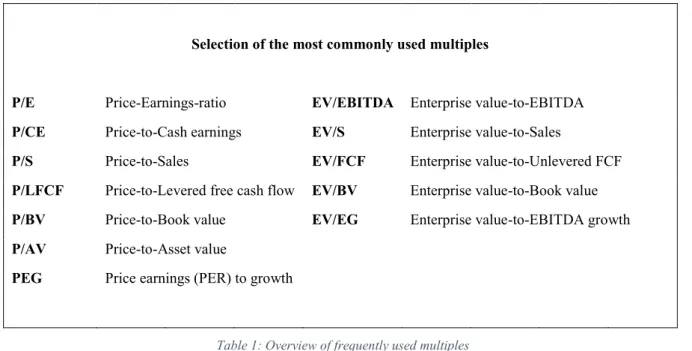
The use of multiples in valuation is an indirect, marked-based valuation approach. The value of an asset is derived from a comparable asset or a synthetic peer group, which is priced and stand-ardized using key statistics such as sales, EBIT, book value among others (Damodaran 2012). Multiples can be the basis of a company valuation or help to precise or validate the result of an intrinsic valuation method (Koller et al. 2005). The first and most critical step is to define an appropriate peer group that has similar characteristics in terms of a companies’ business profile and financial profile. The greater the degree of similarity, the higher the precision of the pro-vided results (Eberhart 2001). In efficient markets, results should be aligned with those of the DCF approach (Damodaran 2006). The second step is to scale the market price to an average key statistic to get a standardized price, as the scale or units may diverge. The third step is to modify certain standardized characteristics between the related assets. For example, companies with higher growth rates normally trade at higher multiple values than companies with lower growth rates (Damodaran 2006; Benninga and Sarig 1997). The most widely used multiples are price multiples and enterprise multiples, as shown below (Fernandez 2001).
15
Selection of the most commonly used multiples
P/E Price-Earnings-ratio EV/EBITDA Enterprise value-to-EBITDA
P/CE Price-to-Cash earnings EV/S Enterprise value-to-Sales
P/S Price-to-Sales EV/FCF Enterprise value-to-Unlevered FCF
P/LFCF Price-to-Levered free cash flow EV/BV Enterprise value-to-Book value
P/BV Price-to-Book value EV/EG Enterprise value-to-EBITDA growth
P/AV Price-to-Asset value
PEG Price earnings (PER) to growth
Table 1: Overview of frequently used multiples
Price multiples are ratios of a share price in the market against the fundamental value per share of a comparable company. Enterprise value multiples include the total market value of all units of a firm’s capital to the measure of the fundamental value of the company as a whole (Pinto et al. 2015). Advantages are, compared to other intrinsic valuation methods, that multiples are faster to apply and less assumptions must be undermined (Damodaran 2006). In addition, mul-tiples are easier to understand and thus, more practical to present to customers (DeAngelo 1990). However, the simplicity itself can be a disadvantage when markets are mispriced. Fur-thermore, finding comparable companies with a similar business profile and financial profile may be an issue. But even with the same characteristics, different accounting policies can result in misinterpretation (Rosenbaum and Pearl 2009). The evidence for the accuracy of estimating the stock prices using multiples is contradicted, but a form of relative valuation is still used in almost 90 percent of equity valuations (Damodaran 2006). For the valuation of PUMA, the most commonly used multiples P/E, EV/Sales, EV/EBITDA and EV/EBIT are applied.
16
3 Global Economy Overview
PUMA is exposed to macroeconomic developments due to its global presence. The company’s performance outcomes are dependent on external factors which are analyzed in this chapter. In the second half of 2018, the global economy weakened noticeably. China changed its regu-latory obstacles for shadow banks and trade tensions began to emerge with the US. The escala-tion of this trade dispute inhibits exposed emerging and developed economies. In Europe, un-certainties such as the Brexit negotiations harmed trade and consumption, new environmental regulations ceased the German automotive industry and rising sovereign spreads in Italy ham-pered investments. The effects of these events are carried into H1 2019 and should normalize in H2 2019. Trade tensions between the US and China are expected to ease, temporary problems in the Euro zone can be tackled and emerging markets, particularly Turkey and Argentina, are expected to stabilize. Moreover, lower taxes in the US and expanding public investments coun-terbalance instabilities. Nevertheless, economists expect the global economy to grow at a slightly lower pace, down from 3.6% in 2018 to 3.3% in 2019. The trend towards stabilization in H2 2019 is anticipated to continue, leading to a global growth of 3.6% in 2020 and around 3.5% beyond, as shown in Figure 1. (IMF 2019)
Figure 1: Real GDP growth 2008 - 2024E
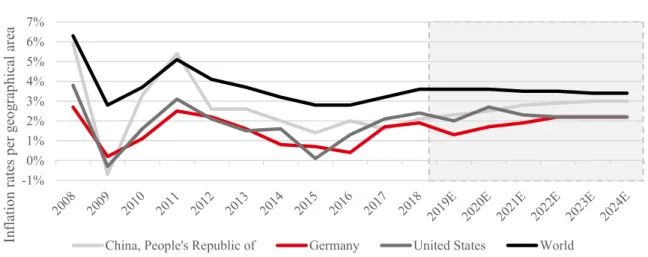
World inflation rates are expected to remain constant with a trend to decrease slightly. Within a geographical breakdown, these inflation rates are used to calculate and predict the growth forecast based on nominal GDP developments.
-6% -4% -2% 0% 2% 4% 6% 8% 10% 12% R ea l GDP g ro w th p er co un tr y
Real GDP growth 2008 - 2024E
17
Figure 2: Inflation rates 2008 - 2024E
PUMA is exposed to currency fluctuations due to its worldwide sales and purchasing (97% of all products are sourced in Asia, where contracts are settled in USD). Since US and German inflation rates are expected to converge to a level of 2.2% in the long run, there is no need for exceptional adjustments for exchange rate risks, assuming that exchange differences are mainly explained by inflation. Beyond that, PUMA is hedging its exchange rate risks with currency forward contracts, accounted under the effective cash flow hedging principle of IAS 39 within the transition phase of IFRS 9.
Future risks are unpredictable consequences of trade tensions mentioned above, the uncertain Brexit result and sovereign yields in Italy that could spread to other European countries. After an upward trend in Q3 2016 the 10-year sovereign bond yields were decreasing again until Q2019, as presented in Figure 3 (Federal Reserve Bank of St. Louis 2019).
Figure 3: 10-Year sovereign bond yield average
0.99% 0.01% 2.57% -1% 0% 1% 2% 3% 4% 5% 2008 2009 2010 2011 2012 2013 2014 2015 2016 2017 2018 2019 Yield p er g eo gr ap hical ar ea Date
10-Year sovereign bond yield average
Euro Area Germany USA -1% 0% 1% 2% 3% 4% 5% 6% 7% In flatio n rates p er g eo gr ap hical ar ea
Inflation rates 2008 - 2024E
18 Compared to past years, interest rates are at a low level with rising yields in the US. The US Federal Reserve signaled to stop interest rate increases for 2019. Other central banks such as ECB, Bank of Japan and Bank of England already moved to a more accommodative monetary police while China’s central bank acts more expansionary due to the trade restrictions. A trend can be seen for the long-term interest rate estimation by the OECD, where US rates are rising significantly (IMF 2019; OECD 2019).
0.00% 1.00% 2.00% 3.00% 4.00% 5.00% 2008 2009 2010 2011 2012 2013 2014 2015 2016 2017 2018 2019 2020 L on g-ter m in ter est rates
Long-term interest rates 2008 - 2020E
Germany USA EA17
-1.00% 0.00% 1.00% 2.00% 3.00% 4.00% 5.00% 2008 2009 2010 2011 2012 2013 2014 2015 2016 2017 2018 2019 2020 Sh or t-ter m in ter est rates
Short-term interest rates 2008 - 2020E
Germany USA EA17
Figure 5: Long-term interest rates 2008 - 2020E Figure 4: Short-term interest rates 2008 - 2020E
19
4 Industry Overview
As a producer and seller of sports footwear, apparel and accessories, PUMA’s defined industry is the sportswear and sports equipment market.
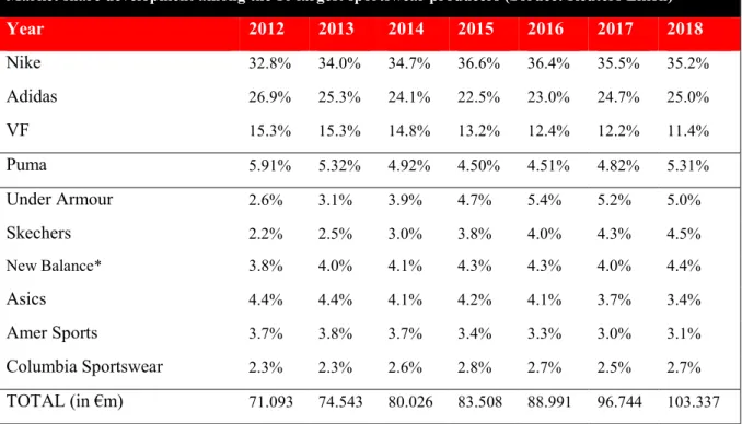
The ten major players in the market include Nike, Inc., Adidas AG, VF Corporation, Puma SE, Under Armour Inc., Columbia Sportswear, Amer Sports Corporation, New Balance Inc., and ASICS Corporation. Among these competitors, Puma has a market share of 5.31%, as illustrated in below. A split of shares in the market is presented in the chart below (Thomson Reuters Eikon 2019).
Figure 6: Market Share of the largest sportswear producers 35.22% 25.01% 11.43% 5.31% 5.03% 4.49% 4.35% 3.39% 3.06% 2.71%
Share of the largest sportswear and sports equipment producers
by sales in 2018
Nike Adidas VF* Puma
Under Armour Scetchers New Balance Asics
Amer Sports Columbia Sportswear
*2017 *2017
20
Market share development among the 10 largest sportswear producers (Soruce: Reuters Eikon)
Year 2012 2013 2014 2015 2016 2017 2018 Nike 32.8% 34.0% 34.7% 36.6% 36.4% 35.5% 35.2% Adidas 26.9% 25.3% 24.1% 22.5% 23.0% 24.7% 25.0% VF 15.3% 15.3% 14.8% 13.2% 12.4% 12.2% 11.4% Puma 5.91% 5.32% 4.92% 4.50% 4.51% 4.82% 5.31% Under Armour 2.6% 3.1% 3.9% 4.7% 5.4% 5.2% 5.0% Skechers 2.2% 2.5% 3.0% 3.8% 4.0% 4.3% 4.5% New Balance* 3.8% 4.0% 4.1% 4.3% 4.3% 4.0% 4.4% Asics 4.4% 4.4% 4.1% 4.2% 4.1% 3.7% 3.4% Amer Sports 3.7% 3.8% 3.7% 3.4% 3.3% 3.0% 3.1% Columbia Sportswear 2.3% 2.3% 2.6% 2.8% 2.7% 2.5% 2.7% TOTAL (in €m) 71.093 74.543 80.026 83.508 88.991 96.744 103.337
*Estimates (private company)
Table 2: Market share development among the 10 largest sportswear producers
The sporting industry is rapidly evolving due to emerging sports technologies and changing trends among the society. Sporting items are discretionary goods. Main growth factor is an increasing health awareness among the population resulting in higher mass sports activities. Large sports events such as the 2018 FIFA World Cup or the Olympic Games are drivers for the sports market success. Public institutions allocating funds for healthcare initiatives, improv-ing the sports infrastructure and organizimprov-ing sport events to spark awareness of the importance of exercise. Trends to use sportswear as casual fashion boost the sportswear market heavily. Moreover, advanced material manufacturing leads to higher adoption rates for customers. More convenient e-commerce and m-commerce distribution channels enhance the willingness to buy sportswear. Additionally, increasing wealth standards in emerging markets enabled people to spend more on leisure activities (Grand View Research 2018, 2018).
However, increased distribution and predilection for indoor activities, such as video games, virtual reality, movies or smartphone usage restrains market growth. (Allied Market Research 2018). Additionally, increasing prices for products have negative impacts on sales. Lastly, counterfeit products harm the sales for brands (Marketline 2019, 2019).
Buyer`s power is moderate in the sports equipment market, especially for strong brands that can sell their products exclusively in their stores. In this case, switching costs are not negligible unless the buyer is satisfied with a substitute product (Marketline 2019). Supplier power varies
21 in the sports equipment market, especially for strong brands. Here, retailers cannot afford to stock up their products (Marketline 2019). The size of the sportswear market is estimated at $300.2bn in 2017, divided into various subcategories (Euromonitor International 2018).
Figure 7: Market size and segment overview
Outlook and Trends
The largest market is currently in North America, accounting for about 35.5% whereas the Asian Pacific market is the fastest growing market, with an expected 8.4% compound annual growth rate (CAGR) due to increasing wealth and health awareness. The following graph illus-trates the regional historical and expected growth rates for sports market industry (Euromonitor International 2018). €1,700m €70m €48m €30m €16m €81m €54m €300m
Market size and segment overview in 2018
Apparel and footwear Sportswear Sports/inspired appared Sports/inspired footwear Outdoor apparel Outdoor footwear Performance apparel Performance footwear
Apparel and Footwear Market
Sports Apparel and Footwear Market
22
Figure 9: Market growth by region
Industry experts estimate the segment ball games including football or basketball to post the highest growth until 2025. In China, Badminton and basketball are the most popular sports (Euromonitor International 2018; Research and Markets 2018). In the last five years, the sports-wear market demonstrate on average growth rates of more than twice than the global real GDP (Euromonitor International 2018; The World Bank 2019).
5.3% 6.1% 4.1% 1.0% 2.0% 3.7% 3.40% 8.45% 4.40% 3.71% 2.49% 4.23% 0% 1% 2% 3% 4% 5% 6% 7% 8% 9%
North America Asia Pacific Western Europe Latin America Middle East & Africa Global Average Ma rk et gr ow th b y ar ea
Market growth by region
CAGR (2017-2012) CAGR (2022-2017) Source: Euromonitor, 2018 0.9x 3.2x 3.6x 2.6x 2.1x 2.4x 2.0x 1.8x 1.4x 1.4x 0.0x 0.5x 1.0x 1.5x 2.0x 2.5x 3.0x 3.5x 4.0x 0% 1% 2% 3% 4% 5% 6% 7% 8% 9% 10%
2013 2014 2015 2016 2017 2018 2019E 2020E 2021E 2022E
Mu ltip ler Gr ow th r ates (I nd us tr y an d rea l G DP )
Global sportswear market vs. real GDP, %Y-o-Y change
Sportswear growth real GDP growth Multiplier
23 The expected CAGR for the global sportswear market is forecasted at 4% until 2022, compared with 2% for the wider fashion industry. While the US is still the main driver for the market with a value growth of $19bn over 2017-2022, the rising key markets are China and India accounting for a combined value growth of $23bn. The sports market is rapidly adapting new technologies such as big data, wearables or sensors for health measurements. New market entries in the sports equipment market is only possible for niche markets focusing on e-retailing to compete against the large players. Another trend is the sustainable fashion through environmental friendly re-sources and production (Euromonitor International 2018; PUMA SE 2019b).
24
5 Company Overview
PUMA at a Glance2PUMA was founded in 1948 and has its headquarters in Herzogenaurach, Germany. The com-pany is listed on the German MDAX and operates as a European Corporation (SE) under the chief executive officer (CEO) Bjørn Gulden. The company is involved in designing, develop-ing, and distributing the segments footwear, apparel and accessories in the sports industry.
Product Line
PUMA´s product line includes sports performance and sportstyle products across six business units: Teamsport, Running, Training, Golf, Motorsport, Sportstyle and Licensing. PUMA dis-tinguishes between Footwear, Apparel and Accessories. The following figures show the contri-bution of each segment to total revenues and the development of revenues per product segment.
Figure 10: Revenue split by segment
Figure 11: Sales across segments
2 Unless otherwise stated, all data processed in this chapter is obtained from the source PUMA SE 2019b
(PUMA´s Annual Report 2018)
17%
36% 47%
Revenue split by segments in FY18
Accessories Apparel Footwear 1,506 1,627 1,975 2,185 1,245 1,333 1,441 1,688 636 667 720 776 €0m €1,000m €2,000m €3,000m €4,000m €5,000m 2015 2016 2017 2018 R ev en ues
Revenues across segments
Accessories Apparel Footwear
25 While footwear represents the largest share in terms of sales, the highest growth segment is apparels with 17.1% compared to footwear and accessories with 10.6% and 7.8%, respectively.
Geographic Mix
PUMA reports its sales as groups of EMEA (39%), Americas (35%) and Asia/Pacific (APAC) (26%). While in 2018 EMEA and Americas have the largest market shares, the Asia/Pacific area has the highest growth rate with 24.2% compared to 9.4% in EMEA and 7.9% in Americas, measured in reporting currency. Figure 12 – Figure 14 give an overview of the sales by geog-raphy.
Figure 12: EMEA sales & growth Figure 13: Americas sales & growth
Figure 14: APAC sales & growth
1,311 1,340 1,495 1,613 23% 2% 12% 8% 0% 5% 10% 15% 20% 25% €0m €500m €1,000m €1,500m €2,000m 2015 2016 2017 2018
EMEA
sales & growth
818 905 995 1,236 8% 11% 10% 24% 0% 5% 10% 15% 20% 25% €0m €500m €1,000m €1,500m €2,000m 2015 2016 2017 2018
APAC sales & growth
1,258 1,383 1,646 1,800 4% 10% 19% 9% 0% 5% 10% 15% 20% 25% €0m €500m €1,000m €1,500m €2,000m 2015 2016 2017 2018
26
Distribution Channels
The distribution channels of its brands PUMA and COBRA Golf are operated through whole-sale (76%) and direct whole-sales (24%) in its own retail stores and online stores.
Figure 15: Distribution channel mix
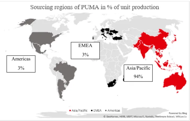
Around 120 countries are within PUMA`s distribution scope. The sourcing organization col-laborates with a worldwide network of independent manufacturers. PUMA’s major sourcing area from production and transport to distribution is based in Asia.
Figure 16: Sourcing regions of PUMA in % of unit production in FY18. 76%
24%
Distribution channel mix by revenue in FY18
Wholesale Direct sales
24% growth in direct sales FY18 16% growth in wholesale FY18 Asia/Pacific 94% EMEA 3% Americas 3%
27 Due to this concentration of sourcing, various factors like third party manufacturers, exchange rate, fluctuations, tax changes, trade restrictions or political instability represents a risk.
However, PUMA’s management is confident to be prepared for potential negative develop-ments through global diversification and alternative scenario planning in case of occurring events. Cross-currency risks of the large exposure of contracts denominated in US Dollar through its product sourcing in Asia are hedged with forward contracts.
Strategy
PUMA’s mission statement “Forever Faster” from 2014 was created to become the “world’s fastest sports brand” and to enable full potential for athletes while expressing their personality and style. Beyond that, the philosophy is valid for the whole product cycle from fast-decision making to production to distribution while ensuring a quick adaption of market trends. The most famous strategic partner to follow these goals is the world record sprinter Usain Bolt. The year 2014 was the year of change and the company followed a strong financial development and a great improvement of their brand awareness. For fiscal year 2019 (FY19) to fiscal year 2021 (FY21), PUMA`s main strategic goals are building a comprehensive offer for women and reen-tering and establishing the basketball market.
Sponsorships
The sponsorship of sports teams and professional athletes is essential for sportswear distributers like PUMA to create a strong brand positioning. PUMA has a mix of sponsoring for athletes, entertainers and professional sports teams. The most famous brand ambassadors are Usain Bolt, Lewis Hamilton, Antoine Griezmann, Rihanna, Selena Gomez and the football teams Arsenal London, Borussia Dortmund, AC Milan and the National Team of Italy, as illustrated below.
28
Figure 18: Sponsorships (b)
Sustainability
Sustainability gains importance in todays’ global society. PUMA has set goals for 10 of the 20 United Nations sustainable development goals:
Figure 19: Sustainability goals
In March 2019, PUMA announced the launch of a sustainable sportswear collection in collaboration with First Mile by using yearn from recycled plastic bottles (PUMA SE 2019a). In April 2019, PUMA finalized its ambitious goals to use 90% sustainable down feathers, leather, cotton and polyester by 2020 with a cooperation of Responsible Down Standards,
29 proclaimed that it reached its previous target of 50% sustainability two years ahead of schedule (PUMA SE 4/23/2019).
Social Media
Social media presence is gaining importance as a key driver of growing brand heat through influencer and ambassadors and thus, to create demand for its products (Aral et al. 2013). Puma has 9.6m Instagram followers with a significant growth of 51% since 1 January 2018 and 20.1m follower on Facebook with a growth of 6% (Trackalytics 2019).
Figure 20: Social media followers
This comparison demonstrates a competitive disadvantage against its main competitors Nike and Adidas in terms of social media awareness and advertising power. Against its smaller com-petitor Reebok that belongs to Nike, PUMA is superior. In recent years, Puma has become a skillful player on social media, generating brand awareness and product demand through its marketing campaigns. 86.9m 32.8m 35.7m 23.4m 9.6m 20.1m 2.3m 9.3m +15% +11% +11% +32% +51% +6% +64% +9% 0% 10% 20% 30% 40% 50% 60% 70% 0m 10m 20m 30m 40m 50m 60m 70m 80m 90m 100m Nike Instagram Nike Facebook Adidas Instagram Adidas Facebook Puma Instagram Puma Facebook Reebok Instagram Reebok Facebook G ro w th ra te from 1 J an 18 -to d ay Social m ed ia fo llow ers
Social media followers (1 Jan 2018 - today)
30
Key Financials
Table 3: Key financial figures
In 2018, PUMA generated a currency adjusted sales increase of 12.4% to €4,648m (17.6% or-ganic growth). The gross profit margin improved by 110 basis points to 48.4%. Its operating expenses increased by 11.8% to €1,928m while the cost-to-sales ratio improved from 41.7% to 41.5%. 75% of the marketing budget was spent for sports and 25% for lifestyle.3 Net earnings
increased by 38% from €135.8m to €187.4m with earnings per share from €9.09 to €12.54. The operating margin improved from 5.9% (€245m) in FY17 to 7.3% (€337m) in FY18.
Figure 21: Sales and EBIT margin
3 Information provided by PUMA’s investor conference in February 2019.
in € m 2014 2015 2016 2017 2018 Trend Sales 2972.0 3387.4 3626.7 4135.9 4648.3 % growth 3.30% 14.0% 7.1% 14.0% 12.4% Gross Profit 1,385.4 1,540.2 1,656.4 1,954.4 2,249.3 % sales 46.6% 45.5% 45.7% 47.3% 48.4% EBITDA 185.8 153.7 187.5 314.9 419.3 % sales 6.3% 4.5% 5.2% 7.6% 9.0% EBIT 128.0 96.2 127.6 244.6 337.2 % sales 4.3% 2.8% 3.5% 5.9% 7.3% Net Income 64.1 37.1 62.4 135.7 187.3 % sales 2.2% 1.1% 1.7% 3.3% 4.0% 2,972 3,387 3,627 4,136 4,648 4.3% 2.8% 3.5% 5.9% 7.3% 0% 2% 4% 6% 8% 10% 12% 14% €0m €1,000m €2,000m €3,000m €4,000m €5,000m 2014 2015 2016 2017 2018 E B IT m ar gin Sales
Sales and EBIT margin
31
Employees
The company employed in FY18 on average 12,192 people compared to 11,389 in FY17, mainly due to the increased number of retail stores. The productivity per employee increased, measured relation of EBIT/FTE and Sales/FTE in the past years.
Figure 22: EBIT vs. EBIT/FTE
Figure 23: Sales vs. Sales/FTE
128 96 128 245 337 11.9 8.8 11.5 21.5 27.7 €0k €5k €10k €15k €20k €25k €30k €35k €40k €0m €50m €100m €150m €200m €250m €300m €350m €400m 2014 2015 2016 2017 2018 E B IT /Em plo yee E B IT EBIT vs. EBIT/FTE
EBIT in €m EBIT/ Employee in €k
2972 3387 3627 4136 4648 276.5 308.3 325.9 363.1 381.3 €0k €100k €200k €300k €400k €500k €0m €1,000m €2,000m €3,000m €4,000m €5,000m 2014 2015 2016 2017 2018 Sales/ FT E Sales Sales vs. Sales/FTE Sales in €m Sales/FTE in €k
32
PUMA Shares
As of 31 December 2018, Puma has a market capitalization of €6.4bn. The share price devel-opment of the last 5 years is visualized below with a current share price of €544.50 on 18 April 2019 and €427.00 on 31 December 2018. The 5-year high is €544.50 (current) and 5-year low was at €142.45. In the past 5 years, PUMA outperformed its index, the MDAX. By looking at the last 3 years, PUMA’s share outperformed the MDAX as well as its main competitors Adidas and Nike. The following graphs illustrate the share price development of PUMA and comparing the quote history with competitors and the index MDAX.
Figure 24: PUMA SE 5-year share price development
The following graphs demonstrate the strong performance of PUMA during the past years. In the last 5 years, PUMA was only outperformed by Adidas. In the last 3 years, PUMA´s stock outperformed Adidas, Nike and the MDAX almost constantly.
142.45 519.00 427.00 544.50 0 100 200 300 400 500 600 P rice in €
33
Figure 25: PUMA SE 5-year share price development compared to the MDAX index
Figure 26: PUMA SE 3-year share price development compared to the MDAX index
In the annual general meeting, the management proposed a dividend of € 3.50 per share for 2018, which is equal to a payout ratio of 27.9%. For 2017, a one-time special dividend was paid as a result of business improvements and to value Kerings’ collaborative effort (PUMA SE 2018). 0% 50% 100% 150% 200% 250% 300% In dex ed s har e pr ice
PUMA SE 5-Year share price development compared to index
MDAX Index Puma Nike Adidas
0% 20% 40% 60% 80% 100% 120% 140% 160% 180% 200% In dex ed s har e pr ice
PUMA SE 3-year share price development compared to index
34
Figure 27: Dividend per share
Ownership structure
In May 2018, PUMA’s majority shareholder, Kering S.A., reduced its share from 86% to 16% as dividend in kind to its shareholders. The reason behind this strategical decision was to fully focus on luxury brands and to offset its “imbalance” and “to avoid a drawn-out disposal of Puma to a third party”, according to Kering’s management (Reuters 2018a). For CEO Gulden, this deal was the “best option” Reuters (2018b). Artemis, holder of 40.9% of Kering’s shares be-comes strategic shareholder with 28.54% ownership. As a result, the public float increased from 13% to 55%. With this new ownership structure, PUMA returned to the German MDAX in June 2018.
Figure 28: Ownership structure
0.5 0.5 0.75 12.5 3.5 € 0 € 2 € 4 € 6 € 8 € 10 € 12 € 14 2014 2015 2016 2017 2018 Div id en d p er sh ar e
Dividend per share
28.8% 15.8% 4.7% 2.4% 2.1% 55.4%
Ownership structure in FY18
Artemis SA Kering SA BlackRock Carmignac Gestion Fidelity International Free Float