Printed version ISSN 0001-3765 / Online version ISSN 1678-2690 http://dx.doi.org/10.1590/0001-3765201820170420
www.scielo.br/aabc | www.fb.com/aabcjournal
Seasonal variations, metal distribution and water quality in the Todos
os Santos River, Southeastern Brazil: a multivariate analysis
CLÁUDIA A.F. PEREIRA1
, LUIZ F.O. MAIA1
, MÁRCIA C.S. FARIA1
, PAULO H. FIDÊNCIO2 , CLEIDE A. BOMFETI1, FERNANDO BARBOSA JUNIOR3 and JAIRO L. RODRIGUES1
1
Instituto de Ciência, Engenharia e Tecnologia, Universidade Federal dos Vales do Jequitinhonha e Mucuri, Rua do Cruzeiro, 01, 39803-371 Teófilo Otoni, MG, Brazil
2
Faculdade de Ciências Exatas e Tecnológicas, Universidade Federal dos Vales do Jequitinhonha e Mucuri, Avenida Diamantina, s/n, 39100-000 Diamantina, MG, Brazil
3
Faculdade de Ciências Farmacêuticas de Ribeirão Preto, Universidade de São Paulo, Avenida do Café, s/n, 14040-903 Ribeirão Preto, SP, Brazil
Manuscript received on June 5, 2017; accepted for publication on April 4, 2018
ABSTRACT
In aquatic habitats, metal contamination from natural and anthropogenic sources continues to pose a concern for human and environmental health. Thus, it is important to complete monitoring studies to assess patterns and the extent of metal contamination in these ecosystems. The purpose of this work was to determine the concentrations of 31 chemical elements and water quality parameters of the Todos os Santos River located in the Mucuri Valley, Minas Gerais, Brazil. A multivariate statistical analysis was used to determine any seasonal and spatial patterns from the data. Results demonstrated that metals including Al, Fe, and Ni exceeded Brazilian and international guidelines nutrients as P also exceed water quality standards. Principal components analysis indicated distinct geographical and seasonal patterns for multiple elements with hierarchical cluster analysis confirming the observed spatial patterns of contamination in the Todos os Santos River.
Key words: toxic pollutants, metals, water quality, environment.
Correspondence to: Jairo Lisboa Rodrigues E-mail: [email protected]
INTRODUCTION
Anthropogenic activities carried out in urban and rural areas generate pollutants that are usually discharged into rivers without prior treatment. These activities include industrial activities, use of pesticides, fertilizers, and manures. Rivers, lakes, and seas have received large amounts of wastewater from domestic and industrial sources,
thus endangering the living beings that use these
water resources on a daily basis (Ohe et al. 2004,
Jordão et al. 2007). Therefore, water bodies may be
contaminated with complex, ill-defined mixtures of
chemicals and most freshwater organisms will be
exposed, to varying degrees, to this contamination
(Scalon et al. 2013). The toxic elements produced
are relocated by the action of rain, contaminating
soils and waterways that surround these areas (Ren
Among the contaminants present in waters, metals stand out. In aquatic environments, metals may come from various natural and anthropogenic sources, such as atmospheric deposition, geological weathering, agricultural activities and residential and industrial products (Weber et al. 2013). High concentrations of these pollutants have been
demonstrated to cause adverse effects in the human
body, such as heart and neurological problems and skin cancer, affecting many ecosystems (Chiba et al.2011, Chang and Ling 2014). The Todos os Santos River (TSR) is located in Teófilo Otoni
(Mucuri Valley, Minas Gerais State, Brazil).
This water system receives a waste discharge of various origins, especially in parts of the river that run through urban areas. However, there are few studies on the environmental conditions of this river and the possible types of contamination that could lead to health risks for the local populations. Recently, a study conducted by Blanc et al. 2014 at the Todos os Santos River pointed out concentrations of aluminum, phosphorus, and iron above the maximum levels permitted by Brazilian law (CONAMA 2005) and the World Health Organization (WHO 2004).
The objective of the present study was to determine the metal concentrations, physical and chemical parameters in TSR water samples during periods of rain and drought, to assess spatial and temporal patterns in water quality using multivariate statistical analyses.
MATERIALS AND METHODS
Samples were taken over a period of eight months in 2012, comprising periods of drought, which include the months from May to September, and the rainy season, which lasts from October to December. Two points are located upstream the selected urban area and near the source of the river (points 1 and 2); two other points are located downstream the urban area (points 5 and 6), and two are located within
the urban area, which is in a region with severe contamination (points 3 and 4). At each sample site, about 1 L of water was collected according to the CETESB standards (CETESB 2012), using metal-free polypropylene bottles. The samples were stored at 4ºC until analysis, and a total sample volume of 100 mL was collected for the physical and chemical analyses.
The geographic coordinates of each point
were determined using a Garmin 60CSx GPS
receiver. The geographical location and altitude of the sampling sites are 17°50’S 41°40’W and 598.4 m 1), 17º48’S 41º39’W and 550.8 m (P-2); 17°51’S 41°30’W and 328.5 m (P-3), 17°52’S 41°29’W 319 m (P-4), 17°52’S 41°27’W and 310 m (P-5); 17°52’S 41°18’W and 272.5 m (P-6). The
water collection points (n=6) were defined based
on several parameters, such as the proximity to urban centers and water use within a radius of 74 km (Fig. 1).
The physical and chemical parameters measured were pH, dissolved oxygen, turbidity, conductivity, and temperature, using a pH-meter (power meter model mPA-210), an oximeter (model DO5519), a turbidimeter (Poly Control, model AP-2000), and a conductivity meter (model mCA – 150p) for conductivity and temperature, respectively. The measurements were made following the instruction manuals of each equipment. The dissolved oxygen, conductivity and temperature were determined in situ, and pH and turbidity were analyzed in the laboratory. High
purity deionized water (resistivity 18.2 M Ω cm)
obtained by the Milli-Q system (Millipore®) was used throughout the study and for preparing the calibration standards.
The determination of metals was performed by an inductively coupled plasma mass spectrometer (ICP-MS, ELAN DRC II, PerkinElmer), according to the method of Lawrence et al. 2006
with modifications. The equipment was installed
to distillation at a temperature below its boiling point using a Quartz distiller (Kürner). High
purity deionized water (resistivity 18.2 M Ω .cm)
obtained by the Milli-Q system (Millipore®) was used throughout the study. Quality control for the determination of metals in the water samples was carried out via analysis of water standard reference materials (Aluminum, Antimony, Arsenic, Barium, Beryllium, Boron, Cadmium, Calcium, Chromium, Cobalt, Copper, Iron, Lead, Magnesium, Manganese, Molybdenum, Nickel, Potassium, Selenium, Silver, Silicon, Sodium, Strontium, Thallium, Uranium, Vanadium, Zinc) from the National Institute of Standards and Technology (NIST 1640, Trace Elements in Natural Water). The reference samples were analyzed before and after ten runs of ordinary
water samples. There were no statistical differences
between the concentration values obtained for the reference materials and the “target-values” for
95% confidence intervals using the T-test. In the
toxicology and properties of metals, Universidade de São Paulo (USP-Brazil). The determination of iron (Fe) levels in the collected samples was carried out with a spectrophotometer (Siqueira et al. 2009). For this, we used a spectrophotometer SP-220-Brazil.
The following metals were tested in surface water samples 107Ag, 27Al, 75As, 138Ba, 9Be, 209Bi, 44
Ca, 111Cd, 59Co, 133Cs, 63Cu, 69Ga, 202Hg, 115In, 39K, 7
Li, 55Mn, 23Na, 60Ni, 31P, 208Pb, 32S, 82Se, 28Si, 88Sr, 205
Tl, 238U, 51V, 184W and 66Zn. The limits of detection (LOD) method for these elements were 0.002; 0.005; 0.0002; 0.003; 0.001; 0.01; 0.0001; 0.001; 0.001; 0.0006; 0.01; 0.0005; 0.009; 0.0007; 0.05; 0.002; 0.0001; 0.005; 0.0009; 0.4; 0.0001; 8.0; 0.001; 0.09; 0.0002; 0.06; 0.0001; 0.001; 0.005 and 0.0008 µg L-1, respectively. For this, were used calibration standard solutions from PerkinElmer (USA).
All reagents used were of analytical quality except high purity HNO3, which was submitted
multivariate analysis, the data were arranged in a matrix consisting of variables (columns), such as
the concentration of each identified constituent; the
objects (rows) were the sampled populations. The matrix was self-scaled before PCA and HCA were performed, the latter using the algorithm of means (Laurence et al.2006). Data were analyzed using chemometrics software in MATLAB version 5.3 and the package PLS_Toolbox (Version 2.0).
RESULTS AND DISCUSSION
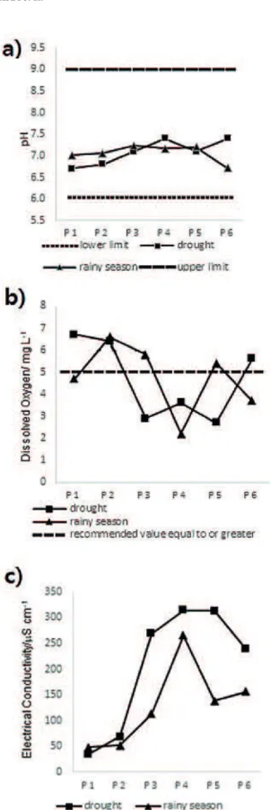
The average results of physical and chemical analyses in periods of drought and rain are shown in Fig. 2. During the dry period, the pH ranged from 6.7 to 7.4, and the turbidity varied between 4.4 and 58 NTU. These values of pH and turbidity are in agreement with the recommendations by the Resolution 357 of CONAMA/2005 (pH from 6.0 to 9.0 and turbidity until 100 NTU). The levels of dissolved oxygen (DO) were in disagreement with the resolution at points P-3, P-4 and P-5, ranging from 2.7 to 6.7 mg L-1.
During the rainy period, the pH and turbidity ranged from 6.7 to 7.2 and 4.8 to 89 NTU, respectively. The DO values in the rainy period ranged from 2.2 to 6.6 mg L-1; locations P-1, P-4, and P-6 were below the established minimum value (5 mg L-1 DO) by the Resolution 357 of CONAMA/2005.
Dissolved oxygen is essential to aquatic life (Jordão et al. 2007), and low values are associated to the presence of oxidable substances, such as biodegradable organic matter and ions of lower oxidation state as Fe (II) and Mn (II) (Von Sperling 1996). This situation can lead to problems for the organisms living in the river because reduced oxygen in the water is not conducive to the survival of aerobic organisms and it is essential for the maintenance of the natural processes (CETESB 2001).
In both seasons, the electrical conductivity of TSR exhibited high values when passing through
the urban perimeter of Teófilo Otoni city (P-3 and
P-4). In the dry season, the values at points P-3,
P-4, P-5 and P-6 ranged from 239 to 314 μS cm-1 . During the rainy season, these same points ranged
from 113 to 265 μS cm-1
. Therefore, 66.7% of the assessed points (P3 to P6) suggested anthropogenic changes in this parameter during the two seasons.
Regarding the physical and chemical parameters, the samples collected in both periods (i.e., drought and rainy) presented similar results for electrical conductivity and turbidity. For dissolved oxygen, similar results were found for locations 3, 4 and 5 during the drought season.
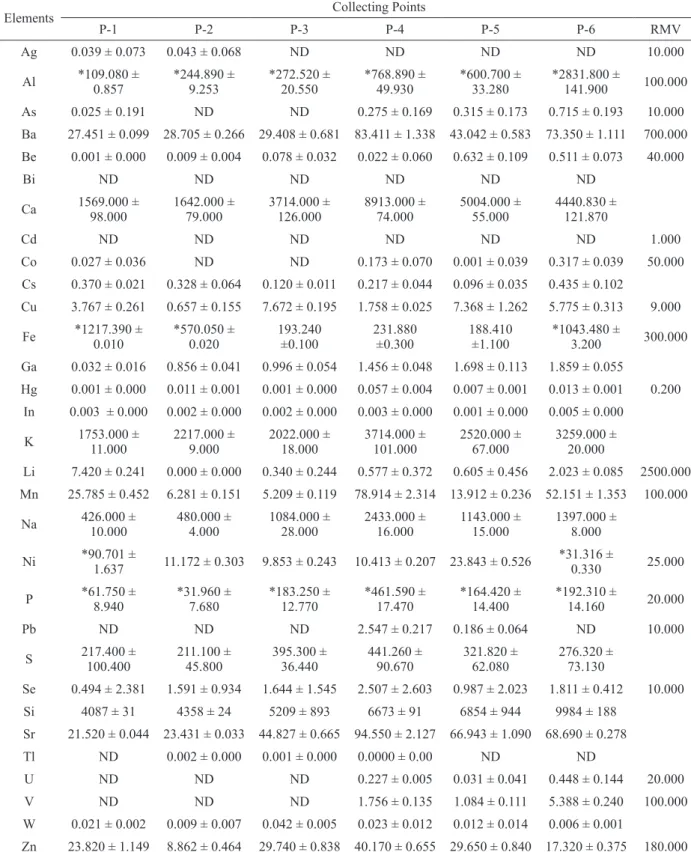
The mean values of trace elements analyzed during the dry and rainy seasons are showed in Tables I and II. It can be seen that the elements aluminum, iron, and phosphorus were above those permitted by local regulations during both periods.
During the dry season, changes in the Al and Fe levels may be due to the inappropriate disposal of solid wastes, which can be observed along the route of the river; alternatively, these elements may be characteristic of the soil in this region. Lixiviation may also be considered given the high concentrations of aluminum. Elevated levels of P are related to domestic waste dumps in the riverbed (Christophoridis et al. 2009) as well as fertilizer used near the river (Rothwell et al. 2011).
In the rainy season, excessive levels of Ni were found. This may have been caused by industrial activities in the region (ATSDR 2005) and even the use of agricultural fertilizers contaminated by
this metal (Campos et al. 2005), causing significant
amounts of these contaminants to be eliminated in the river.
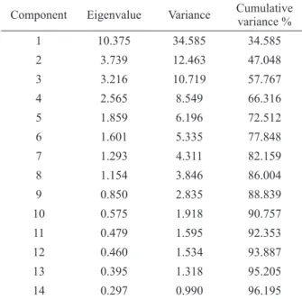
Matlab software was used to discover principal components (PCs) on water metal concentration series. Table III presented all the PCA eigenvalues for these water metals, and Table IV showed the corresponding principal component loadings. According to Table III, two PCs were selected and
the first principal component (PC1) was a measure
of all elements less than Cr, Ni, Se, Ag and Hg which are indicative of primary contaminants; the second principal component (PC2) was primarily attributed
to all elements less than Cd, Na, Be, Hg, Ag, Ta, Ga,
Bi, In, Fe, P and S which is indicative of a second contaminant. In this way, the dataset resulted in two PCs, explaining 47.05% of the variance. These two independent principal components seemed to dominate the contamination data.
We performed an exploratory analysis using principal components analysis (PCA) and hierarchical cluster analysis (HCA), as shown in Fig. 3, in which the letters identify the collection month (i.e., A, May; B, June; C, July; D, September; and E, December). Fourteen principal components explained 96.2% of the variance. The PC1 and PC2 components accumulated the higher variances
and were used for the differentiation of samples
from the collection sites. The other components of accumulated minor variances were not enough to
differentiate samples from collection sites. Thus,
the sample in the PCA was grouped into six groups
(G1 to G6). In this way, we can identify whether
the samples collected in the month of December exhibited any similarities, as indicated by their position at the top (i.e., positive) part of PC2, which explained 12.5% of the total variance, and the left (i.e., negative) part of PC1, which explained 34.6%.
TABLE I
Mean values of trace element concentrations in water samples during the dry season (sample concentration ± standard deviation in µg L-1
). RMV in µg L-1
(Recommended Maximum values according to CONAMA 2005).
Elements Collecting Points
P-1 P-2 P-3 P-4 P-5 P-6 RMV
Ag 1.640 ± 0.178 0.973 ± 0.167 0.431 ± 0.062 0.379 ± 0.038 0.104 ± 0.014 0.128 ± 0.051 10.000 Al 27.870 ± 4.160 *455.280 ±
24.050 *447.080 ± 78.960 *233.950 ± 19.690 *721.530 ± 182.150 689.970 ± 73.900 100.000 As 0.156 ± 0.038 0.173 ± 0.051 0.289 ± 0.088 0.342 ± 0.082 0.516 ± 0.121 0.334 ± 0.066 10.000 Ba 20.540 ± 0.253 33.540 ± 0.375 36.510 ± 2.362 63.430 ± 9.676 56.060 ± 4.595 40.220 ± 0.407 700.000 Be 0.001 ± 0.000 0.064 ± 0.068 0.078 ± 0.048 0.032 ± 0.120 0.411 ± 0.203 0.642 ± 0.140 40.000 Bi 0.011 ± 0.004 0.016 ± 0.006 0.020 ± 0.007 0.013 ± 0.006 0.020 ± 0.005 0.023 ± 0.004
Ca 897.000 ± 86.000 2762.000 ± 239.000 11045.000 ± 654.000 12655.000 ± 766.000 13158.000 ± 171.000 8629.000 ± 347.000
Cd 0.001 ± 0.003 0.005 ± 0.011 0.014 ± 0.005 0.017 ± 0.007 0.024 ± 0.013 0.016 ± 0.062 1.000 Co 0.018 ± 0.007 0.061 ± 0.010 0.432 ± 0.043 0.353 ± 0.031 0.329 ± 0.046 0.231 ± 0.012 50.000 Cs 0.258 ± 0.006 0.302 ± 0.010 0.239 ± 0.023 0.270 ± 0.012 0.290 ± 0.034 0.218 ± 0.016
Cu 0.139 ± 0.028 0.162 ± 0.045 1.600 ± 0.060 0.656 ± 0.050 1.190 ± 0.247 7.357 ± 0.043 9.000 Fe *881.200 ±
1.200 *1281.700 ± 2.100 *2484.300 ± 2.200 *3425.900 ± 1.700 *5945.600 ± 1.600 *3239.300 ± 1.700 300.000 Ga 0.528 ± 0.029 1.013 ± 0.048 1.079 ± 0.087 1.632 ± 0.054 1.900 ± 0.211 1.376 ± 0.068
Hg 0.027 ± 0.008 0.019 ± 0.003 0.003 ± 0.011 0.031 ± 0.005 0.012 ± 0.004 0.017 ± 0.002 0.200 In 0.006 ± 0.003 0.005 ± 0.001 0.006 ± 0.002 0.006 ± 0.001 0.005 ± 0.001 0.006 ± 0.003
K 357.000 ±
8.000 1106.000 ± 64.000 4565.000 ± 506.000 5360.000 ± 157.000 6759.000 ± 849.000 5834.000 ± 193.000 Li 0.309 ± 0.144 0.475 ± 0.181 1.008 ± 0.280 345.974 ±
0.948 2.568 ± 0.211 2.478 ± 0.093 2500.000 Mn 15.720 ± 0.210 28.880 ± 1.360 66.040 ± 2.490 134.000 ±
4.110
181.670 ±
15.800 70.220 ± 1.940 100.000 Na 2033.000 ±
70.000 3345.000 ± 182.000 12525.000 ± 1690.000 15892.000 ± 808.000 17228.000 ± 2684.000 23958.000 ± 587.000
Ni 0.280 ± 0.410 0.910 ± 0.058 1.780 ± 0.132 1.810 ± 0.154 1.140 ± 0.140 1.510 ± 0.099 25.000
P *25.800 ±
10.810 *103.600 ± 11.100 *841.900 ± 24.800 *612.730 ± 14.178 *1167.590 ± 24.600 *269.030 ± 15.110 20.000 Pb 0.018 ± 0.013 0.098 ± 0.015 2.175 ± 0.176 3.670 ± 0.090 2.014 ± 0.270 0.875 ± 0.250 10.000
S 281.800 ±
141.200 281.400 ± 68.400 417.500 ± 57.580 412.200 ± 80.300 366.945 ± 70.600 294.200 ± 92.130
Se 1.145 ± 1.481 0.962 ± 1.546 0.564 ± 0.161 2.146 ± 1.411 1.592 ± 1.157 0.543 ± 1.452 10.000 Si 3585.000 ±
128.000 4873.000 ± 120.000 8499.000 ± 155.000 10299.000 ± 211.000 9502.000 ± 223.000 10699.000 ± 287.000 Sr 14.970 ± 0.152 28.994 ± 0.397 62.250 ± 2.020 82.570 ± 1.600 73.370 ± 4.500 43.050 ± 0.817 Tℓ 0.015 ± 0.004 0.044 ± 0.008 0.017 ± 0.002 0.027 ± 0.006 0.015 ± 0.004 0.015 ± 0.005
U 0.004 ± 0.005 0.116 ± 0.020 0.096 ± 0.016 0.191 ± 0.015 0.163 ± 0.040 0.192 ± 0.023 20.000 V 0.031 ± 0.002 0.883 ± 0.026 0.748 ± 0.088 1.679 ± 0.079 2.059 ± 0.343 1.598 ± 0.295 100.000 W 0.025 ± 0.005 0.012 ± 0.003 0.057 ± 0.003 0.018 ± 0.008 0.035 ± 0.014 0.020 ± 0.008
TABLE II
Mean values of trace elements in water samples during the rainy season (sample concentration ± standard deviation in µg L-1
). RMV in µg L-1
(Recommended Maximum Values according to CONAMA 2005).
Elements Collecting Points
P-1 P-2 P-3 P-4 P-5 P-6 RMV
Ag 0.039 ± 0.073 0.043 ± 0.068 ND ND ND ND 10.000
Al *109.080 ± 0.857 *244.890 ± 9.253 *272.520 ± 20.550 *768.890 ± 49.930 *600.700 ± 33.280 *2831.800 ± 141.900 100.000
As 0.025 ± 0.191 ND ND 0.275 ± 0.169 0.315 ± 0.173 0.715 ± 0.193 10.000
Ba 27.451 ± 0.099 28.705 ± 0.266 29.408 ± 0.681 83.411 ± 1.338 43.042 ± 0.583 73.350 ± 1.111 700.000 Be 0.001 ± 0.000 0.009 ± 0.004 0.078 ± 0.032 0.022 ± 0.060 0.632 ± 0.109 0.511 ± 0.073 40.000
Bi ND ND ND ND ND ND
Ca 1569.000 ± 98.000 1642.000 ± 79.000 3714.000 ± 126.000 8913.000 ± 74.000 5004.000 ± 55.000 4440.830 ± 121.870
Cd ND ND ND ND ND ND 1.000
Co 0.027 ± 0.036 ND ND 0.173 ± 0.070 0.001 ± 0.039 0.317 ± 0.039 50.000
Cs 0.370 ± 0.021 0.328 ± 0.064 0.120 ± 0.011 0.217 ± 0.044 0.096 ± 0.035 0.435 ± 0.102
Cu 3.767 ± 0.261 0.657 ± 0.155 7.672 ± 0.195 1.758 ± 0.025 7.368 ± 1.262 5.775 ± 0.313 9.000 Fe *1217.390 ±
0.010 *570.050 ± 0.020 193.240 ±0.100 231.880 ±0.300 188.410 ±1.100 *1043.480 ± 3.200 300.000 Ga 0.032 ± 0.016 0.856 ± 0.041 0.996 ± 0.054 1.456 ± 0.048 1.698 ± 0.113 1.859 ± 0.055
Hg 0.001 ± 0.000 0.011 ± 0.001 0.001 ± 0.000 0.057 ± 0.004 0.007 ± 0.001 0.013 ± 0.001 0.200 In 0.003 ± 0.000 0.002 ± 0.000 0.002 ± 0.000 0.003 ± 0.000 0.001 ± 0.000 0.005 ± 0.000
K 1753.000 ± 11.000 2217.000 ± 9.000 2022.000 ± 18.000 3714.000 ± 101.000 2520.000 ± 67.000 3259.000 ± 20.000
Li 7.420 ± 0.241 0.000 ± 0.000 0.340 ± 0.244 0.577 ± 0.372 0.605 ± 0.456 2.023 ± 0.085 2500.000 Mn 25.785 ± 0.452 6.281 ± 0.151 5.209 ± 0.119 78.914 ± 2.314 13.912 ± 0.236 52.151 ± 1.353 100.000
Na 426.000 ± 10.000 480.000 ± 4.000 1084.000 ± 28.000 2433.000 ± 16.000 1143.000 ± 15.000 1397.000 ± 8.000 Ni *90.701 ±
1.637 11.172 ± 0.303 9.853 ± 0.243 10.413 ± 0.207 23.843 ± 0.526
*31.316 ±
0.330 25.000
P *61.750 ±
8.940 *31.960 ± 7.680 *183.250 ± 12.770 *461.590 ± 17.470 *164.420 ± 14.400 *192.310 ± 14.160 20.000
Pb ND ND ND 2.547 ± 0.217 0.186 ± 0.064 ND 10.000
S 217.400 ±
100.400 211.100 ± 45.800 395.300 ± 36.440 441.260 ± 90.670 321.820 ± 62.080 276.320 ± 73.130
Se 0.494 ± 2.381 1.591 ± 0.934 1.644 ± 1.545 2.507 ± 2.603 0.987 ± 2.023 1.811 ± 0.412 10.000 Si 4087 ± 31 4358 ± 24 5209 ± 893 6673 ± 91 6854 ± 944 9984 ± 188
Sr 21.520 ± 0.044 23.431 ± 0.033 44.827 ± 0.665 94.550 ± 2.127 66.943 ± 1.090 68.690 ± 0.278
Tl ND 0.002 ± 0.000 0.001 ± 0.000 0.0000 ± 0.00 ND ND
U ND ND ND 0.227 ± 0.005 0.031 ± 0.041 0.448 ± 0.144 20.000
V ND ND ND 1.756 ± 0.135 1.084 ± 0.111 5.388 ± 0.240 100.000
W 0.021 ± 0.002 0.009 ± 0.007 0.042 ± 0.005 0.023 ± 0.012 0.012 ± 0.014 0.006 ± 0.001
3 collected in May, area 5 in June, location 6 in July and location 4 in May. Regarding the samples with negative values of PC1 and positive values of PC2, this group of samples comprises those from point 2 collected in July, location 3 in June and September, area 4 in July, location 5 in May, July, and September and point 6 in July.
This distribution of water samples collected at different locations and in different months is
explained by influences on the elemental content,
as represented in the graph of weights (Fig. 4). In the positive region of PC2 and negative region of
PC1, the elements that have the strongest influence are Ni, Cr, and Se. The influence of Ag, Hg, and In
is strong in the region in which both PC1 and PC2 are negative. When PC1 and PC2 are both positive, the elements Cu, Li, Ce, Zn, Al, Sr, Ba, Ur, Va, As, Pb, K, Co, Ca and Mn stand out. For the region in which PC2 is negative and PC1 is positive, clustering is due to the levels of Be, Na, Cd, P, Fe,
Ta, Bi, Ga and S.
CONCLUSIONS
The levels of dissolved oxygen during the dry and rainy period were in desagreement with the
local regulations for points 3, 4, 5. The electrical conductivity of TSR exhibited high values in both seasons for points 3 and 4.
During the dry season the metals aluminum (points 2, 3, 4, 5) and iron (points 1-6) are outside the range permitted. For rainy season, aluminum (points 1-6), iron (points 1, 2, 6) and nickel (points 1, 6) exhibited high levels. The nonmetal phosphorus was found in disagreement with the legislation in the 6 points analysed for both seasons.
TABLE III
Eigenvalues of PCA for water metal analysis datasets.
Component Eigenvalue Variance Cumulative variance %
1 10.375 34.585 34.585
2 3.739 12.463 47.048
3 3.216 10.719 57.767
4 2.565 8.549 66.316
5 1.859 6.196 72.512
6 1.601 5.335 77.848
7 1.293 4.311 82.159
8 1.154 3.846 86.004
9 0.850 2.835 88.839
10 0.575 1.918 90.757
11 0.479 1.595 92.353
12 0.460 1.534 93.887
13 0.395 1.318 95.205
14 0.297 0.990 96.195
TABLE IV
Data for principal components 1 and 2 of the water analysis datasets.
Components PC1 PC2
Cr -0.113 0.4183
Mn 0.270 0.0062
Co 0.260 0.0301
Cu 0.025 0.1855
Pb 0.223 0.0269
Cd 0.248 -0.0140
Li 0.075 0.1542
Al 0.162 0.2544
Na 0.180 -0.1006
Ba 0.216 0.1750
K 0.241 0.0298
As 0.245 0.1077
Be 0.110 -0.0155
Hg -0.060 -0.1735
Ni -0.081 0.3595
Ag -0.060 -0.1574
Se -0.042 0.0191
Ta 0.100 -0.2274
Ur 0.217 0.1388
Zn 0.117 0.2575
Va 0.234 0.1902
Ga 0.259 -0.2083
Sr 0.162 0.0764
Bi 0.182 -0.2222
Ca 0.276 0.0223
Ce 0.077 0.0616
In -0.017 -0.2016
Fe 0.254 -0.0866
P 0.249 -0.0244
Exploratory analysis using PCA and HCA demonstrated that are similarities among samples
collected in different months at various locations,
and together with the other dates, it can be suggest that TSR is facing a contamination problem that
can influence the living beings that depends of this
water source to survive.
ACKNOWLEDGMENTS
The authors are grateful to Fundação de Amparo à
Pesquisa do Estado de Minas Gerais (FAPEMIG), Conselho Nacional de Desenvolvimento Científico
e Tecnológico (CNPq), Fundação de Amparo à Pesquisa do Estado de São Paulo (FAPESP), Rede
Mineira de Química (RQ-MG), Movimento Pró Rio
Todos os Santos e Mucuri (MPRT SM) and Comitê
de Bacia Hidrográfica do Rio Mucuri (CBH-MU1) for financial support and fellowships.
REFERENCES
ATSDR - AGENCY FOR TOXIC SUBSTANCES AND DISEASE REGISTRY. 2005. Toxicological Profile for Nickel. Available at: http://www.atsdr.cdc.gov/toxprofiles/ tp15.pdf. Accessed in 27/08/2015.
BLANC LR, MOREIRA FS, GONÇALVES AM, MANCHESTER RSS, BARONI L, FARIA MC DA S, BOMFETI CA, BARBOSA F AND RODRIGUES JL. 2014. Contamination in a Brazilian River: A Risk of Exposure to Untreated Effluents. J Environ Qual 42: 1596-1601.
CAMPOS MR, DA SILVA FN, NETO AEF, GUILHERME LRG, MARQUES JJ AND ANTUNES AS. 2005. Determination of cadmium, copper, chromium, nickel, lead and zinc in rock phosphates. Pesq Agropec Bras 40: 361-367.
CETESB - COMPANHIA AMBIENTAL DO ESTADO DE SÃO PAULO. 2001. Relatório de Qualidade das Águas Interiores do Estado de São Paulo. São Paulo, Brasil. CETESB - COMPANHIA AMBIENTAL DO ESTADO DE
SÃO PAULO. 2012. Guia Nacional de Coleta e Preservação de Amostras. Disponível em: http://laboratorios.cetesb. sp.gov.br/wp-content/uploads/sites/47/2013/11/guia-nacional-coleta-2012.pdf.
CHANG C AND LING Y. 2014. A water quality monitoring network design using fuzzy theory and multiple criteria analysis. Environ Monit Assess 186: 6459-6469.
CHIBA WAC, PASSERINI MD, BAIO JAF, TORRES JC AND TUNDISI JG. 2011. Seasonal study of contamination by metal in water and sediment in the sub-basin in the southeast of Brazil. Braz J Biol 71: 833-843. C H R I S T O P H O R I D I S C , D E D E P S I D I S D A N D
FYTIANOS K. 2009. Occurrence and distribution of selected heavy metals in the surface sediments of Thermaikos Gulf, N. Greece. Assessment using pollution indicators. J Hazard Mater 168: 1082-1091.
CONAMA - CONSELHO NACIONAL DO MEIO AMBIENTE. 2005. Resolução Nº. 357, Ministério do Meio Ambiente: Brasília, Brasil.
J O R D Ã O C P, R I B E I R O P R , M AT O S AT A N D FERNANDES RBA. 2007. Aquatic Contamination of the Turvo Limpo River Basin at the Minas Gerais State, Brazil. J Braz Chem Soc 18: 116-125.
Figure 3 - Scores of water samples collected in different months based on the metal content of the Todos os Santos River.
Figure 4 - Loadings representing the influence of different
LAWRENCE MG, GREIG A, COLLERSON KD AND KAMBER BS. 2006. Direct quantification of rare earth element concentrations in natural waters by ICP-MS. Appl Geochem 21: 839-848.
OHE T, TATSUSHI W AND KEIJI W. 2004. Mutagens in surface waters: a review. Mutat Res-Rev Mutat 67: 109-149.
REN S, MEE RW AND FRYMIER PD. 2004. Using factorial experiments to study the toxicity of metal mixtures. Ecotoxicol Environ Saf 59: 38-43.
R E Z E N D E P S, M O U R A PA S, D U R Ã O J R WA, NASCENTES CA, WINDMOLLER CC AND COSTA LM. 2011. Arsenic and Mercury Mobility in Brazilian Sediments from the São Francisco River Basin. J Braz Chem Soc 22: 910-918.
ROTHWELL JJ, DISE NB, TAYLOR KG, ALLOTT THE, SCHOLEFIELD P, DAVIES H AND NEAL C. 2011. A spatial and seasonal assessment of river water chemistry across north west England. Sci Total Environ 408: 841-855.
SCALON MCS, RECHENMACHER C, SIEBEL AM, KAYSER ML, RODRIGUES MT, MALUF SW, RODRIGUES MAS AND DA SILVA LB. 2013. Genotoxic Potential and Physicochemical Parameters of Sinos River, Southern Brazil. Sci World J 2013: 1-7. SIQUEIRA LFS, COSTA NETO JJG AND ROJAS MOAI.
2009. Determination of iron (II) in seawater by Fe system (II)/KSCN via UV-Vis spectrometry: a low-cost and practical alternative, Universidade Federal do Maranhão: São Luís, MA, Brasil.
VON SPERLING M. 1996. Introdução à Qualidade das Águas e ao Tratamento de Esgotos, 4a
ed., Belo Horizonte: UFMG, 452 p.
WEBER P, BEHR ER, KNORR CL, VENDRUSCOLO D S , F L O R E S E M M , D R E S S L E R V L A N D BALDISSEROTTO B. 2013. Metals in the water, sediment, and tissues of two fish species from different trophic levels in a subtropical Brazilian river. Microchem J 106: 61-66.