A non-Invasive method to determine the contribuition of mono and bi-articular torque during the knee extension

Texto

(1)A Non-Invasive Method to Determine the Contribution of Mono and Bi-articular Torque During the Knee Extension. Fellipe de Tácio do Nascimento Diniz Porto, 2015.

(2)

(3) A Non-Invasive Method to Determine the Contribution of Mono and Bi-articular Torque During the Knee Extension. Dissertation submitted to the Faculty of Sport, University of Porto to obtain the 2nd cycle in High Performance Sport, under the degree-law nº 74/2006, 24th March.. Orientador: Professor Doutor Filipe Conceição. Fellipe de Tácio do Nascimento Diniz Porto, 2015.

(4) Ficha de Catalogação. Diniz, F. T. (2015). A Non-Invasive Method to Determine the Contribution of Mono and Bi-articular Torque During the Knee Extension. Porto: Diniz, F. Master Thesis in High Performance Sport presented to the Faculty of Sport, University of Porto.. Keywords: Muscle contribution, bi-articular muscles, mono-articular muscles, force-length relationship, biomechanics. IV.

(5) DEDICATÓRIA. Para meus pais, meus avós (in memoriam), minha irmã, minha família e todos os meus verdadeiros amigos. V.

(6) VI.

(7) AGRADECIMENTOS. Aos meus pais, que me proporcionaram essa e outras oportunidades na vida, e por todo amor dado a mim.. A minha irmã por sempre está ao meu lado me orientando e apoiando em minhas decisões.. Aos meus avós (in memoriam) que sempre me amaram e foram de fundamental importância para minha vida.. A minha namorada, que sempre me apoiou e esteve ao meu lado nos momentos difíceis.. Ao meu primo/irmão Romullo que sempre esteve comigo me fortalecendo e ajudando nos momentos ruins.. Aos meus primos e tios que me mostraram o real valor do amor em família.. Ao meu orientador Professor Doutor Filipe Conceição, por permanecer várias horas disponível para me ajudar e esclarecer minhas dúvidas além de me contagiar com seu impressionante bom humor.. Ao Professor Mestre João Carvalho, por toda paciência que teve comigo, pela ajuda e orientação no desenvolvimento dessa tese.. Ao meu amigo e Professor Mestre Vanthauze Marque que me ajudou bastante na em toda minha jornada em busca do conhecimento.. Aos membros amigos do clube de atletismo, Escola do Movimento (ESCMOV), que me receberam de braços abertos.. VII.

(8) Aos atletas participantes em meus amigos, que estavam sempre disponíveis para me auxiliar no que fosse preciso.. Aos meus amigos de verdade, que sempre me apoiaram e estiveram ao meu lado.. VIII.

(9) General Index. DEDICATÓRIA. V. AGRADECIMENTOS. VII. General Index. IX. Index of Figures. XI. Index of Equations. XIII. List of Abbreviation. XV. Resumo. XVII. Abstract. XIX. CHAPTER I - INTRODUCTION. 1. 1.1 Introduction. 3. 1.2 Structure of the Dissertation. 4. CHAPTER II – LITERATURE REVIEW. 5. 2. Skeletal Muscle. 7. 2.1. Muscle Anatomy. 7. 2.1.1. Muscular Fiber Types. 9. 2.1. Muscle Architecture. 10. 2.3. Muscle Action Classification. 11. 2.4. Tendon Anatomophysiology. 11. 2.5. Mono and Bi-articular Muscles. 12. 2.6. Mechanical Muscle Model. 14. 2.6.1. Hill Muscle Model. 14. 2.6.1.1. Contractile Element Properties. 14. 2.6.1.1.1. Force-Length Relationship. 15. 2.6.1.1.2. Force-Velocity Relationship. 18. 2.6.1.2. Series Elastic Element. 19. 2.6.1.3. Parallel Elastic Elements. 20. 2.7. Isokinetic Dynamometer. 20 IX.

(10) 2.8. Muscle Moment Arm. 21. 2.9. Muscle Contribution for Knee Extension. 24. CHAPTER III – MATHERIALS AND METHODS. 27. 3. Materials and Methods. 29. 3.1. Joint Toque Measure. 30. 3.1.1. Dynamometer Measures. 30. 3.1.2. Procedures to Determine Isometric Mono and Bi-articular Muscle Torque. 31. 3.1.3. Procedures to Determine Isokinetic Mono and Bi-articular Muscle Torque. 37. CHAPTER IV – RESULTS. 39. 4. Results. 41. 4.1. Isometric Contraction Results. 41. 4.2. Isokinetic Results. 46. CHAPTER V – DISCUSSION. 47. 5. Discussion. 49. CHAPTER VI – CONCLUSIONS. 53. 6. Conclusions. 55. CHAPTER VII – BIBLIOGRAPHY. 57. 7. Bibliography. 59. X.

(11) Index of Figures. Figure 1. Skeletal Muscle Organization. 8. Figure 2. Muscle myofibrils. 9. Figure 3. Pennate muscle. A: unipennate (vastus lateralis); B: bipennate (rectus femoris); C: multipennate (deltoid). 10. Figure 4. Tendon structure. 12. Figure 5. Hill type. 14. Figure 6. Theoretical muscle force-length relationship curve. 15. Figure 7. Force-length relationship of human flexors. 16. Figure 8. Sarcomere force-length. 17. Figure 9. Velocity-load relationship. 18. Figure 10. Force-velocity curve. 19. Figure 11. Joint alterations. 22. Figure 12.a Knee muscles length. 22. Figure 12.b Knee muscles moment arm. 22. Figure 13.a Hip muscles length. 22. Figure 13.b Hip muscles moment arm. 22. Figure 14. Angles orientation. 23. Figure 15. Quadriceps view, rectus femoris. 24. Figure 16. Quadriceps view, vastus. 24. Figure 17. Schematic representation of mono and bi-articular muscle behavior. 33. Figure 18. Soluble system of equation. 34. Figure 19. Solution of the system of equation. 34. XI.

(12) Figure 20. Simplified solution of the system of equations. 34. Figure 21. Mono Articular knee force. 35. Figure 22. Bi-articular Knee force. 36. Figure 23.a, b, c, d, e and f. Total, calculated, mono and bi-articular torque plot. 41. Figure 24.a, b, c, d, e and f. Mono-articular muscle force plot. 43. Figure 25.a, b, c, d, e and f. Bi-articular muscle force plot. 44. Figure 26. Mono-articular muscle force and torque plot. 45. Figure 27. 3D representation of knee extensors as a function of knee and hip joint angle. 46. XII.

(13) Index of Equations. Equation 1. 21. Equation 2. 31. Equation 3. 31. Equation 4. 31. Equation 5. 32. Equation 6. 32. Equation 7. 32. Equation 8. 36. Equation 9. 36. XIII.

(14) XIV.

(15) List of Abbreviations. PCSA. Physiologic Cross-Sectional Area. CE. Contractile Element. SEE. Series Elastic Element. PEE. Parallel Elastic Element. EL. Equilibrium Length. FL. Force-Length Relationship. L. Length. L0. Length of the Active Muscle Force Peak. F. Muscle Force. F0. Peak Active force. FV. Force-Velocity Relationship. T. Torque. b. Moment Arm. RF. Rectus Femoris. VL. Vastus Lateralis. VM. Vastus Medialis. VI. Vastus Intermedius. BFL. Biceps Femoris Long Head. ST. Semitendinosus. SM. Semimembranosus. GR. Gracillis. AS. Sartorius. BFS. Biceps Femoris Short Head. GL. Gastrocnemius Lateral. GM. Gastrocnemius Medial. PT. Plantaris. PP. Popliteus. XV.

(16) XVI.

(17) Resumo. O presente estudo teve o intuito de desenvolver um método não invasivo para determinar o contributo dos grupos musculares mono-articular (vasto lateral, vasto medial e vasto intermédio) e bi-articular (recto femoral) no movimento de extensão da perna num dinamômetro isocinético. Também foram avaliadas a curva de força/torque-comprimento/ângulo para determinar a gama de ação desses músculos durante este movimento. Este estudo foi desenvolvido com seis atletas velocistas masculinos (22 ± 2 idade, 1.70m ± 0.20m altura, 65kg ± 7kg peso) que realizaram 21 contrações isométricas máximas considerando sete ângulos do joelho (12º,24º,36º,48º,60º,72º e 84º) e três ângulos do quadril (85º, 70º e 55º) e 90 contrações isocinéticas concêntricas em seis diferentes velocidades angulares (45º/s, 60º/s, 90º/s, 120º/s, 150º/s e 180º/s) para os mesmos ângulos do quadril. O torque dos grupos musculares mono e bi articulares foram obtidos através de um sistema matemático solúvel, que decompunha o torque total em torque do grupo muscular mono-articular e torque do grupo muscular bi-articular. A análise do comportamento desses grupos musculares efectuou-se através das curva torque-ângulo tendo sido constatado que o grupo muscular, bi articular, é o maior gerador de torque na articulação do joelho quando o mesmo está nas posições mais estendidas, sendo que, à medida que esta articulação vai fletindo a magnitude do torque do grupo biarticular diminui. Contrariamente para o grupo mono-articular o torque apresenta maior magnitude, quando a articulação do joelho está nas posições mais fletidas, sendo este grupo o principal responsável pela maior geração de torque durante a extensão do joelho. Verificou-se que este método permite uma boa representação dos dados experimentais e a sua decomposição para a obtenção do contributo do grupo mono e bi-articular para o torque total numa grande parte da gama do movimento.. XVII.

(18) XVIII.

(19) Abstract. This study was aimed to develop a non-invasive method for determining the contribution of mono-articular muscle group (vastus lateralis, vastus medialis and vast intermediate) and bi-articular (rectus femoris) on the leg extension movement performed in an isokinetic dynamometer. Also it was evaluated the force/torque-length/angle curve to determine the range of action of these muscles during this movement. This study was conducted with six male sprinters athletes (22 ± 2 years old, 1.70m ± 0.20m high, 65kg ± 7kg weight) who performed 21 maximal isometric contractions considering seven knee angles (12º, 24º, 36º, 48º, 60º, 72º and 84º) and three hip angles (85º, 70º and 55º) and 90 concentric isokinetic contractions in six different angular velocities (45°/s, 60º/s, 90º/s, 120º/s, 150º/s and 180º/s) for the same angles of the hip. The mono and biarticular muscle groups joint torque were obtained using a mathematical soluble system that decomposed the total joint torque at mono and bi-articular muscle group torque. The analysis of these muscle groups behaviors was made through the torque-angle curve. It was found that the bi-articular muscle group is the major torque generator in the knee joint when it is in the most extended positions, and, as this joint flexes the bi-articular group torque magnitude decreases. In contrast to the bi-articular muscle group torque, the mono-articular group torque shows greater magnitude when the knee joint is in the most flexed position, being this group the mainly responsible for the higher torque generation during knee extension. It was found that this method allows a good representation of the experimental data and its decomposition allow to obtain the contribution of mono and bi-articular group torque for a large part of the range of motion.. XIX.

(20) XX.

(21) CHAPTER I INTRODUCTION.

(22) 2.

(23) 1.1. Introduction Nowadays the, in vivo, human biomechanical muscles behavior is still a challenge for the research. Better knowledge of human muscles behavior could provide advantages in the observation of the human movement, understanding of injuries, and help in the control and improvement of the movement. An alternative way to try to understand the muscle behavior is the neuromuscular skeletal model developed by Hill (1938), which subdivided the muscle tendon complex in three elements, (i) contractile element (CE), (ii) series elastic element (SEE) and (iii) parallel elastic element (PEE). Based on the knowledge of the CE it is possible to determine musculoskeletal mechanical proprieties as the forcelength and force-velocity relationship, stiffness, etc. Through these properties, it is possible to better understand the human biomechanical muscle behavior. Since these mechanical properties allow to draw the muscle force, torque and angle behavior throughout a given joint movement. The bi-articular muscle behavior also still challenging for the researches. Even being studied in early times by Galen (131-201 Anno Domini) some of these muscles characteristics are still a dare. The range of action in a given joint movement is also a challenging characteristic, since it is dependent on the joint position which is related with the muscle moment arm, number of joints crossed, making difficult its understanding. The behavior of the mono-articular muscles namely the range of action force production and distribution of the net torques produced still not very clear, considering this behavior is not similar to the biarticular muscles and sometimes they must share this torques along the range of action. Thus, the study of these muscle characteristics is of fundamental importance to better understand the human movement. Therefore the aim of this study was to develop a subject specific non-intrusive technique to determine the contribution of the mono and bi-articular muscle during the knee extension movement from experimental data obtained in an isokinetic dynamometer.. 3.

(24) 1.2. Structure of the Dissertation This dissertation is organized as follows: Chapter I (Introduction) – It was developed a general presentation of the work, developed in this study its purpose and its structure. Chapter II (Literature Review) – This chapter deals with the literature review of the human muscle-tendon complex and its organization, to better clarify the goals and statements of this study. Chapter III (Materials and Methods) – Relates to the materials and the methods used to perform this study. It is this chapter the subjects were characterized and the procedures of this dissertation presented. Chapter IV (Results) – This chapter deals with the presentation of the results obtained from the experimental and theoretical calculation. Chapter V (Discussion) – In this chapter the major results obtained in this study considering the literature review presented are critical discussed. Chapter VI (Conclusions) – In this chapter are showed the major conclusions found in this study, based in the evidences observed in the Chapter V. Chapter VII (Bibliography) – This chapter show the bibliography used as the basis for this work.. 4.

(25) CHAPTER II LITERATURE REVIEW.

(26) 6.

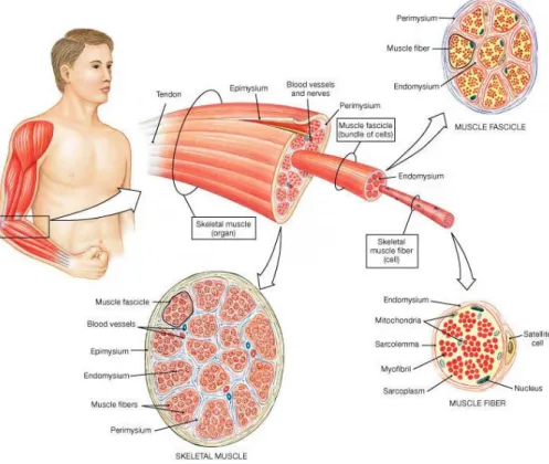
(27) 2. Skeletal Muscle. Responsible for approximately 40% of the human body weight, skeletal muscles have three important functions: (i) generate force for locomotion and breathing, (ii) postural stabilization of the body, and (iii) produce heat for survival when the human body is exposed to environmental stress (Powers, 2009). These skeletal muscles generally originates from a bone or dense connective tissue and inserts at other bone (Fernandes & Petrinelli, 2011). Tendons are the structures who link muscles to the bones and they are composed by a collagenous tissue which make them able to support muscle strains (Maffulli et al., 2004).. 2.1. Muscle Anatomy. The skeletal muscles are composed by long muscles cells, called muscle fibers, which are multinucleated. Each fiber has an external layer of conjunctive tissue (endomysium) who separates the fiber of the others parallels one. However connecting them together, below the endomysium and surrounding the muscles fiber there is a layer of protective tissue called external lamina. Fascicle are bundles of fibers and they are connected by another layer of conjunctive tissue the perimysium. Finally the fascicle set, build the muscles, and the muscles are covered by another connective tissue, the epimysium (Powers, 2009) (Figure 1). Each muscle fiber has a cellular membrane called sarcolemma inside which we found the sarcoplasm, the muscle cytoplasm, where are the myofibrils, cellular proteins and organelles. Between the external lamina and the sarcolemma, there is a group of cells who are called, satellite cells (Powers, 2009). These cells have an important role in the muscles growth and repair. When stimulated they proliferate, merge and mature, thus repairing or developing new cells(Yamada & Bueno Júnior, 2009).. 7.

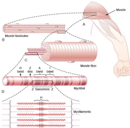
(28) Figure 1. Skeletal Muscle Organization (Martini, 2007). With fusiform structure, the myofibrils are composed by two types of filaments, the thick and the thin ones that are built by two major types of contractile proteins, the myosin and the actin respectively. Also surrounding the actin filaments can be located two others proteins, troponin and tropomyosin, that have a special function in the muscle contraction. The proteins filaments has a specific arrangement who give a striated appearance to the skeletal muscle, and can be subdivided into individual segments, the sarcomeres, that are divided among themselves by a structural protein sheet called Z line or Z disk. At the sarcomeres, it can be observed two different colored portion, the dark and the light. The dark one, called A band, is where the myosin filaments are primarily positioned, while actin filaments are located primarily in the light portion, as known as I band (Powers, 2009) (Figure 2).. 8.

(29) Figure 2. Muscle myofibrils, adapted from Guyton & Hall (2006). 2.1.1. Muscular Fiber Types. In general, the skeletal muscle fiber can be rated in three types, the fibers that are considerate slow and the fast, that are subdivided in two types. These ratings are given due to the biochemical and contractile properties of the skeletal muscles (Powers, 2009). The slow fibers, also known as Type I fibers, are called because of the large oxidative capacity. They contain large numbers of oxidative enzymes, large volume of mitochondria and myoglobin, and are surrounded by a larger number of capillaries than the others fibers. However, when related to the contractile properties, type I fibers have a slower shortening velocity, produce a lower specific tension and are more efficient (require less energy to execute a given work) when compared to the fast fibers (Powers, 2009). The fiber Type II (fast fibers), as mentioned, are subdivided in two forms: Type IIa and Type IIx (Powers, 2009). These nomenclatures are given due to heavy chain of the myosin molecule, which are found in the fibers(Andersen & Aagaard, 9.

(30) 2010). The fibers type IIx are the fast fibers, and have specific characteristics. Their specific tension is greater than the type I fibers, the shortening velocity is highest and the efficiency is lower than the other fibers. The intermediate fibers (type IIa) contain biochemical characteristics between the fibers type I and type IIx, the specific tension of this fiber are similar of the fast fibers, and the they are adaptive fibers that can be molded by the training characteristics (Powers, 2009).. 2.2. Muscle Architecture. The muscle architecture can be defined as the geometrical arrangement related with the position of the muscles fibers, associated to the axis of force generation (Lieber, 1992; Lieber & Fridén, 2000) . The muscle fibers which extends parallel to the axis of force generation are defined as having a parallel architecture muscles (Lieber & Fridén, 2000). Pennate muscles has oblique muscle fibers attachments to the line of muscle action.. Figure 3. Pennate muscle. A: unipennate (vastus lateralis); B: bipennate (rectus femoris); C: multipennate (deltoid) (Muscolino, 2013). The fibers may predispose in different architectural arrangement, thus characterized the muscles as parallels; unipannate, where the oblique fibers are. 10.

(31) attached to one side of the aponeuroses, bipennate, fibers attaching obliquely on to both side of the line of action; and multipennate, where the fibers are attached to two or more branching of a major tendon (Tosovic et al., 2012) (Figure 3). Recent studies showed that the pennation angle and the fascicle length have influence in muscle shortening velocity. When compared sprinters to long distance runners it was found that the sprinters have a longer fascicle length and smaller pennation angle (Abe et al., 2000). Another important aspect of the muscle architecture is the Physiologic CrossSectional Area (PCSA) which correspond to the total cross-sectional areas of all fibers of a specific muscle (Powers, 2009) and can be calculated by the division of the muscle volume by the muscle fiber length (Friederich & Brand, 1990). Muscles with larger PCSA lean to contain a larger proportion of fast fibers, thus allowing a fast shortening of the muscle (Burkholder et al., 1994).. 2.3. Muscle Action Classification. The muscular system can be classified by the function performed in each joint. Muscles that together execute a joint movement are called agonists, the muscle group who opposite to the action of the agonist muscles are known as antagonists, and there is synergists muscle those who assist the agonists. The synergists muscles can help the agonists in two ways, (i) giving extra power to the agonist muscles to perform their movements and (ii) reduce unnecessary and undesirable movements, in order that the agonist muscles can perform movements with greater ease (Marieb, 2009).. 2.4. Tendon Anatomophysiology. Tendons are structures, mainly, composed by collagen and elastin embedded in a proteoglycan-water matrix, who attached the muscles to the bones, and are responsible for the transmission of force generated by muscles to the bones to make the movements possible (Kannus, 2000). 11.

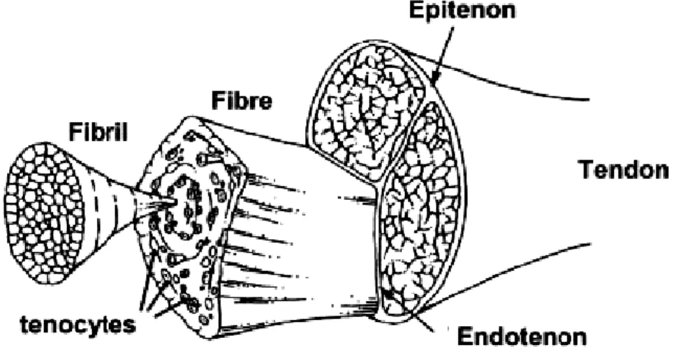
(32) The tendon comprises 65-80% of collagen (the majority being type I), 1-2% of elastin in its composition, what remains consists on tenocytes, tenoblasts, which are among the collagen fibers. Also a fundamental substance, composed by proteoglycans, glycosaminoglycans, structural glycoproteins and other small molecules. Others inorganics components, such as calcium that is found in greater quantity on the dry tendon, representing less than 0.2% of the dry mass of the tendon (Weinreb et al., 2014). The agglomerate collagen fiber form subfascicles that are surrounded by a thin network of connective tissue made by crossed collagen fibril, called endotendon. The subfascicles bundles built the fascicle, who are equally surrounded by the endotendon. Consequently the bundle of fascicle compose the third fiber bundles, also surrounded by the endotendon. Finally the agglomerated of the third fiber bundles originates the tendon itself, that are surrounded by a connective tissue sheath, called epitendon (Figure 4).. Figure 4. Tendon structure (Vieira et al., 2007). 2.5. Mono and Bi-articular Muscles. The skeletal muscles can cross one or more joints. Muscles who just cross one single joint are classified as mono-articular muscles. Thereby muscles that cross two joints are called bi-articular muscles (Carroll & Biewener, 2009). The importance of bi-articular muscles (two-joint muscles) has been discussed since 12.

(33) Galen's (131-201 Anno Domini), who discussed in his work the effect of rectus femoris in hip flexion and knee extension (Kuo, 2001). The distal portion of these muscles are longs and have the length of the full segment, some of them have long tendons and relative short muscles fibers with large pennation angle. Through this profile the bi-articular muscles can be able to support high tension and therefore storage and release elastic energy during the stretch–shortening cycle (Zatsiorsky & Prilutsky, 2012). On the other hand most of the proximal bi-articular muscles have a different profile, having long muscles fibers, small pannation angle and relative short tendons (Zatsiorsky & Prilutsky, 2012). Bi-articular muscles have specific characteristics, when compared to the monoarticular muscles, one of them is the bi-articular muscles can produce motion on the two joints it crosses (Enoka, 2015; Winters et al., 2012). Thus, as the biarticular muscles are performing movements in two joints, the shortening of theses muscles are higher than for corresponding mono-articular muscles. By other side the ability of bi-articular muscles to generate maximum forces is lower than the mono-articular muscle (Bauer, 2004). Other characteristic is that the two joints muscles can transport muscle torque, joint power and mechanical energy throughout the limb (Enoka, 2015; Winters et al., 2012).This energy is not developed by the bi-articular muscles itself but by the mono-articular muscles. And this energy transport can cross the joints in the proximal-distal direction as well in the distal-proximal direction (Bauer, 2004). The force-length and force-velocity of a mono-articular muscle is directly associated to the angle and the angle velocity of the joint that it crosses, whilst the bi-articular muscles force-length and force-velocity depends on the two joints crossed. If the muscle is performing movements in both joint and the joint angular velocity is appropriated the two joints muscles can be acting isometric or eccentric, a different form of the mono-articular muscle (Chapman, 2008).. 13.

(34) 2.6. Mechanical Muscle Model. 2.6.1. Hill Muscle Model. The Hill muscle model is a neuromuscular skeletal model which can predict, through mathematical equations, the muscle force production (Conceição, 2004). The Hill type is basically made by three muscle elements: a contractile element (CE), a series elastic element (SEE), and a parallel elastic element (PEE) (Figure 5). The CE is referred to the muscle part of force generation, the active part of the muscle complex in other words the sarcomere. The SEE and PEE are the passive part of the muscle, so the tendon, aponeurosis and non-active muscle fibers (Rosen et al., 1999). The force that can be generated by the contractile element, depends on the length and the muscle shortening velocity (Zajac, 1989). This part of the system are responsible by the muscle relationships, force-length and. force-velocity. (Conceição, 2004).. Figure 5. Hill type, adapted from Herzog & ter Keurs (1988). 2.6.1.1. Contractile Element Properties. The muscle can be at passive or active state. Therefore passive state is a term given to muscles which are isolated and non-stimulated or also muscles that are in situ at rest (Zatsiorsky & Prilutsky, 2012). The equilibrium length (EL) is a term given to these isolated passive muscles, but it can be also the length of a muscle. 14.

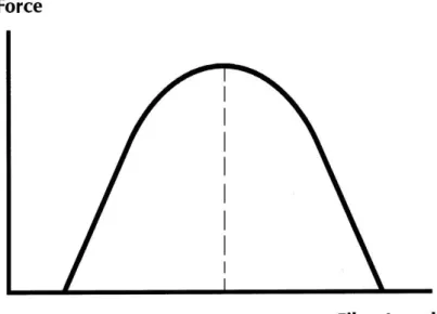
(35) without a mechanic load, and the natural length of a muscle in situ is known as rest length (Zatsiorsky & Prilutsky, 2012). Through a load the muscle can stretch beyond its resting length, and thus providing a passive resistance to this stretch, this resistance do not necessitate metabolic energy (Zatsiorsky & Prilutsky, 2012). When a muscle is stretched beyond its equilibrium length, it resist stretching and produce a passive force. Active muscle force is the term given to the difference in the force developed between the active and the passive muscle, (Conceição, 2004; Zajac, 1989). If there is a muscle activation, the force is increased due to the active force, and the some of these forces are assumed as the total muscle force (Zatsiorsky & Prilutsky, 2012).. 2.6.1.1.1. Force-Length Relationship. The force-length relationship (FL) is an important skeletal muscle propriety, which can predict the muscle isometric maximum force, as a function of muscle fiber length (Conceição, 2004). Through this it is possible to say that the force-length relationship depends on the length of the myosin and actin chains in the muscle sarcomere (Herzog & ter Keurs, 1988).. Figure 6. Theoretical muscle force-length relationship curve. 15.

(36) The active force-length curve is characterized through the muscle length change with the increasing of the force produced, until it reach the maximal the maximal force, after this the force decreasing if the muscle length remain changing. The muscle length which the force is maximum is known as the optimal length (Zatsiorsky & Prilutsky, 2012) (Figure 6). Through the isometric FL curve is likely define the static steady state of the muscle tissue. The FL curve can be analyzed when the muscle fiber is complete activated and its length (L) is constant. The part which can be excited is known as active part, and the other part that can not be excited is called inactivated or passive (Conceição, 2004; Zajac, 1989) . The area where the active force is generated is 0.5L0 < L < 1.5L0, (L0 = length of the active muscle force peak), thus can be said that the muscle force is equal to the peak active force (F = F0) when the muscle fiber length is equal to the length where the muscle generate the active force peak (L = L0). Therefore L0 is called optimal muscle fiber length (Zajac, 1989).. Figure 7. Force-length relationship of human flexors, adapted from Zatsiorsky (2008). Another feature of force-length curve is that when the activation is the same, the muscle can generate highest forces at longer length than the shorter lengths,. 16.

(37) hence theses muscles are considerate as muscles who act at the ascendant limb of the FL curve (Zatsiorsky & Prilutsky, 2012) (Figure 7). Figure 8 show the theoretical sarcomere force-length curve, based on the crossbridge theory of force generation that are results of different overlapping extent between the actin and myosin filaments through the sarcomere length (Zatsiorsky & Prilutsky, 2012).. Figure 8. Sarcomere force-length (Zatsiorsky & Prilutsky, 2012). Where, at the ascending limb (1-2 and 2-3) the myosin and actin overlap the actin filaments from a sarcomere of opposite side, thus decreasing the cross-bridge formation to force generation. The plateau region (3-4) is the region where there are the largest numbers of cross-bridge, thus making possible greater force generation. This area is where the sarcomere is in its optimum length. The descending limb (4-5) is where the myosin and actin filaments are more widely spaced, and it also prevents the cross-bridges formation, so in this area, the force generation is lower.. 17.

(38) For bi-articular muscles, the force-length curve can be estimated by changing the angle of one joint that it crossed and thereby measuring the maximal joint torque at the other joint. The torque of the bi-articular muscle, rectus femoris, should change if the subject tested is sitting in 90º hip angle and in another angle higher, if the muscle is acting in the rising limb of the curve the torque generated by this muscle should improve (Zatsiorsky & Prilutsky, 2012).. 2.6.1.1.2. Force-Velocity Relationship. The force-velocity relationship (FV) can be expressed by the following sentence: with the larger loads shortening begins somewhat later than with the light loads (Fenn & Marsh, 1935). Through this sentence is possible to known that when the loads are high the velocity is low, thus when the loads are light the velocity higher, and when velocity is zero, i.e. occurs an isometric contraction, the force that can be applied can be considered as maximal voluntary force (Hill, 1938) (Figure 9).. Figure 9. Velocity-load relationship. adapted from Edman (2008). The Hill’s curve of force velocity is obtained by an interpolation of force and velocity data recorded in many trials, where the one of these parameters is systematically changed (Zatsiorsky & Prilutsky, 2012). For movements which. 18.

(39) mobilize several muscles the force velocity curve may show different patterns and joint moments arms, however the curve still being descending and concave upward for the muscles which are used. But exceptions are noted in specific cases, for knee extension at low velocities the force which is real generated is lower than that who can be expected for the Hill’s force-velocity relationship, and this relationship, which can partly be explained by inhibition of the knee extensors to prevent injury (Zatsiorsky & Prilutsky, 2012) Other feature of FV relationship, is that this relation is leveled around the maximum isometric force that a muscle can produce where there is a proportion who if the velocity changes 2% the force will change 30%. When occurs a contraction with negative velocity, lengthening contractions (i.e. eccentric contraction) the force performed is around 40% greater than the maximum isometric contraction (Enoka, 2002) (figure 10).. Figure 10. Force-velocity curve (Hall, 1991). 2.6.1.2. Series Elastic Element. The SEE are composed by tendon and aponeurosis, is responsible for the transfer of the force produced in the contractile element to the bones. However, they also are able to optimize the force generated by the CE, through the storage and subsequent release of elastic energy; it is possible since SEE, can elongate. 19.

(40) to storage the elastic energy and release this elastic energy when the muscle shortening (Lewis, 2011). The amount of the elastic energy which the SEE can storage an release is dependent of the stiffness, the maximal force the CE is able to develop in a specific length and the elongation of it (Zatsiorsky & Prilutsky, 2012). Due to be connected to the contractile components, the stiffness of the series elastic components and hence the quantity of elastic energy, which can be storage, depend of the tension that the contractile element can generate and not of the muscle length (Zatsiorsky & Prilutsky, 2012).. 2.6.1.3. Parallel Elastic Elements Composed by various connective tissues, which surround the muscle, sarcolemma, perimysium, epimysium and endomysium. The parallel elastic elements as well as the series elastic elements can generated elastic force but these forces are related to the length of the contractile elements (Lewis, 2011). 2.7. Isokinetic Dynamometer. The isokinetic dynamometer is a highly used tool to measure the torque around a joint, exerted by a given group of muscles. It can measure dynamic forces (concentric and eccentric contractions) or static force (isometric contraction) (Brown et al., 2007). Although the isokinetic dynamometer is widely used, their data can show some problems, the joint torque is one of them, because the results obtained are the sum of the actions of agonist and antagonist muscles. Another problem is related to the acceleration of the crank arm. Until the dynamometer archives the preset velocity its need to accelerate and this can be considered as part of the isokinetic velocity. In the end of the acceleration phase there are some points of velocity overshoot, which also cannot be considered as part of the isokinetic velocity (Lewis, 2011).. 20.

(41) 2.8. Muscle Moment Arm. As definition, muscle moment arm is the perpendicular distance between the line of force production and the axis of the joint that it crosses (Conceição, 2004). However, the muscle moment arm also is an anatomical characteristic that transform the muscle force exerted throughout the movement to a muscle moment of force, through the following equation:. 𝑇𝑜𝑟𝑞𝑢𝑒 = 𝑀𝑜𝑚𝑒𝑛𝑡 𝐴𝑟𝑚 ∙ 𝐹𝑜𝑟𝑐𝑒. (1). Looking to different muscles, those with longer moment arms show better conditions to produce higher torques (T), than muscles with smaller moment arm (b). Even being able to produce higher torques, the muscles with longer moment arms, when producing high angular velocities, they show smaller joints moments, joint power and joint work, which can be explained by the FV relationship (Nagano & Komura, 2003). Changes in the bi-articular muscles length can be observed when changes occurs in one of the joint or in both joints that this muscle crosses. For the biarticular muscles which cross the knee and hip joints, particularly the extensor rectus femoris, when knee joint angle changes, greatest changes in length are observed than when hip joint angle changes. However for the flexor muscles, namely the hamstrings, the behavior is reverse i.e. greater length changes occurs when hip joint angle changes compared to the knee joint angle changes (Visser et al., 1990). Changes in the moment arm are explained by the joint geometry, because the human joints are extensive and not point like, they are no perfectly spherical. Thus, the distance between the bone and the axis center is variable, due to the articular surfaces of the bones, who shows some irregularities, and for the joint cartilage that are composed by visco-elastic substances which deforms with loads, and this leads to changes in the muscle moment arm (Figure 11).. 21.

(42) Figure 11. Joint alterations (Bullough, 2004). In the study developed by Conceição (2004) it was presented the behavior of the mono and bi-articular muscle concerning the length and moment arm changes in a given subject (Figures 12.a, 12.b, 13.a and 13.b). 0.6. 0.04. Moment Arm (m). 0.5. Muscle Length (m). 0.06. vastus rectus Knee hamstrings gastrocnemius. 0.4 0.3. 0.2. 0.02. 0. -0.02. 0.1. -0.04. 0. -0.06. -0.1 0. 20. 40. 60. 80. 100. 120. vastus Rectus knee hamstrings gastrocnemius. -0.08. 140. 0. 20. 40. Knee angle (º). 60. 80. 100. 120. Figure 12.a. Figure 12.b. Figure 12.a Knee muscles length. Figure 12.b Knee muscles moment arm. 0.8. 0.08 0.06. Moment Arm (m). Muscle Length (m). 0.1. gluteus iliopsoas rectus hip hamstrings hip. 0.7 0.6. 0.5 0.4 0.3. 0.04 0.02 0 -0.02 -0.04 -0.06. 0.2. gluteus iliopsoas rectus Hip hamstrings Hip. -0.08. 0.1 -120. -100. Figure 13.a. -80. -60. -40. -20. Hip angle (º). Figure 13.a Hip muscles length. 0. 140. Knee angle (º). 20. -0.1 -120. -100. Figure 13.b. -80. -60. -40. -20. 0. Hip angle (º). Figure 13.b Hip muscles moment arm. 22. 20.

(43) To better understand these figures, the referential used were defined as follows: a) The origin of all angles is the anatomical position b) The angles are measured from the distal segment to the segmental extension of the proximal segment (internal angle), being positive if counter-clockwise (Figure 14).. Figure 14. Angles orientation. Figures 12.a and Figure 12.b represents the performance of the mono-articular (vastus), and bi-articular (rectus) muscles that acts in the knee joint. It can be see the changes that occurs in the rectus femoris length and moment arm. It is possible to see the increase of the length throughout the knee flexion as well as increases in the moment arm. For a small change in the moment arm, greatest changes can be observed in the muscle length. For the vastus the relationship between the length and the moment arm has similar behavior where small changes in the moment arm imply great changes in the muscle length. Based in the referential used if we look to the Figure 13.a the moment arm is negative for all the muscles acting in the flexion of the trunk on the thigh, while those who straightening the trunk their moment arm are positive. Looking to the hamstring in the hip, when angle increases the moment arm is positive and the muscle length decreases. Figure 13.a and 13.b, also represents changes in the rectus femoris length for the hip joint, although the moment arm seems to be quite the same along the movement with changes in the hip angle. 23.

(44) 2.9. Muscle Contribution for Knee Extension. The knee extension is a movement performed by the quadriceps muscles, which includes rectus femoris (RF), vastus lateralis (VL), vastus medialis (VM), and vastus intermedius (VI) (Milner, 2008) (figure 15 and 16). The rectus femoris is the only bi-articular muscle that acts to perform the knee extension being the mono articular muscles the most important in this task.. Figure 15. Quadriceps view, rectus femoris (Mansfield & Neumann, 2014). Figure 16. Quadriceps view, vastus (Mansfield & Neumann, 2014). Concerning the knee flexion the main actuators are the bi-articular muscles (biceps femoris long head (BFL), semitendinosus (ST), semimembranosus (SM), gracillis (GR) and sartorius (SA)), although some relevant role is played by some mono-articular muscles (biceps femoris short head (BFS) gastrocnemius lateral (GL), gastrocnemius medial (GM), plantaris (PT), popliteus (PP)). Through. mechanical. properties. (force-length. relationship,. force-velocity. relationship and their parameters) it is possible to predict the mono and biarticular muscle contribution for the knee extension. Herzog & ter Keurs (1988). 24.

(45) showed in their paper, which tried to determine the human rectus femoris forcelength relationship, that its contribution to the knee extension is approximately 11 – 14%. This data were obtained by comparison between experimental data and the theoretical calculation considering cross-bridges theory, which allows the estimation of the force-length relationship. Lewis (2011) estimates, the muscle contribution to the knee extension from muscles moment arm,. PCSA and. pennation angle, stating that major contribution comes from the three monoarticular muscles. He founds 82.5% contribution of the mono articular muscles being the remainder 17.5% comes from the RF. Pavol & Grabiner (2000) found in their paper, in which they considered only two hip angles (0º and -80º), that RF contribution was also 17% and the average knee extension torque changed, decreasing 7 – 10% between hip joint angles what was unexpected. To the muscles which perform the knee flexion, the major contribution comes from the bi-articular muscles with 62.8% of the knee total torque and the remain 38.2% contribution are from the mono-articular muscles (Lewis, 2011). The same researcher, compared the muscle contribution obtained from data of different researchers with that one of his own experimental data measurements and concludes that the mono and bi-articular contribution of the knee extensor and flexors depends on the hip and knee joint kinematic. Changes in the angle of these two joints will cause variations in the contribution of bi-articular muscles that can vary from 28% to no contribution in the extensors and for the flexors, it can vary from 52% to 100% of the contribution. In this same context looking to the plantar flexion, Sale et al. (1982) observed that the plantar flexion torque was also dependent on the knee angle. These researchers showed that the plantar flexion torque are higher when the knee joint is fully extended compared to knee joint flexed at approximately 90º, and they pointed that these changes are due to the contribution of the bi-articular muscle. In most recent study Conceicao et al. (2012) reinforced this idea and shows that to the bi-articular muscles GL and GM do not perform any force while the knee joint is flexed between 45º and 110º because these muscles are slack. However,. 25.

(46) as the knee angle increases the bi-articular muscles contribution increases reaching up to 65% of the total torque contribution in the angle joint.. 26.

(47) CHAPTER III MATHERIALS AND METHODS.

(48) 28.

(49) 3. Materials and Methods. The aim of this study was to develop a subject specific non-intrusive technique to determine the contribution of the mono and bi-articular muscle during the knee extension movement from experimental data obtained in an isokinetic dynamometer. Thereby, knowing that the knee extension is a movement that involves several muscle groups acting, agonist, antagonist and synergists as well as with some change in the movement plane assumptions were made to group all the force exerted in only one mono-articular (vastus) and bi-articular (rectus) muscles. Therefore, five assumptions/simplifications have been made:. 1. The antagonists’ muscles have an insignificant contribution to the total torque; 2. The agonists can be grouped and represented by two muscles – a monoarticular (Vastus) which represents the grouping of the all three vastus (VL, VM and VI). and a bi articular one (RF) - with filiform tendons that. represents the total/average properties of the muscles of the group (total force, average tendon length and moment arm, etc.); 3. The contribution of small muscles (e.g. popliteus) were ignored; 4. Out of the sagittal plane torques are small and were discarded; 5. Transitory. energy. recycling. (shortening-lengthening. cycles). were. discarded.. Where the first and the fifth simplifications are the most radical regarding most non-laboratory human movement, since in most of them the antagonists muscles have a special role in the energy transferring. Moreover, in the agonists torque generation, the antagonist can act as a regulator of the joint velocity forcing the agonists to perform highest torque to remain the velocity constant. However, in a laboratorial circumstance these variables can be controlled.. 29.

(50) The second simplification has an important meaning in this work, because we give up on knowing the detailed contribution each mono-articular muscles (VL,VM and VI) due to the difficulties in obtaining the data, so we just observed the behavior changing of mono and bi-articular muscles as only two muscles. The third and fourth assumptions are those that have less impact, and it can be explained by the small PCSA which consequently will cause at a lower capacity to generate torque. Thus, five participants took part in the data collection for this study. The subjects were males of national sprinters level, with 22 ± 2 years old males, height 1.70 m ± 0.20 m height, 65kg ± 7kg mass, with experience of using isokinetic dynamometers. 3.1. Joint Toque Measure. 3.1.1. Dynamometer Measures. To obtain the muscular contribution at a given joint movement is necessary to use a non-intrusive technic which is possible to find the muscular torque, and the tool chosen was an isokinetic dynamometer. The knee torques were measured by using a Biodex Multi-Joint System Pro isokinetic dynamometer (Biodex Corporation, Shirley, New York) running the proprietary software. Twenty one isometric contractions were performed at seven different knee angles (12º, 24º, 36º, 48º, 60º, 72º and 84º), and three different hip angles (85º, 70º and 55º) with intervals of one minute and thirty seconds between each trial and ten minutes between each set. The maximum torque for each trial was selected for the analysis. For the isokinetic data collection, six angular velocities, 45º/s, 90º/s, 120º/s,150º/s and 180º/s were selected. For each velocity five concentric and eccentric contractions were performed, at the three different hip angles, 85º, 70º and 55º, both selected in a randomly manner, with one minute and thirty seconds rest. 30.

(51) between each change of angular velocity and ten minutes for each change of hip angle. The maximum torque at each configuration was retained for analysis.. 3.1.2. Procedures to Determine Isometric Mono and Bi-articular Muscle Torque. Assuming that mono and bi-articular muscular group can perform force independently, it is possible to determine the torque-angle curve for both of these muscles by torque decomposition. This decomposition may be possible through the knowledge of muscle length, which can be obtained as a function of the knee and hip angle, either from bibliography or by direct ultrasound measurements. To determine the torque for each muscle group the moment arm is also needed and it can be obtained from the muscle length (equation 2).. 𝑏𝑘𝑛𝑒𝑒 =. 𝜕𝐿 𝜕𝜃𝑘𝑛𝑒𝑒. (2). The total torque is the sum of the torques from each muscle group that act around at a given joint (equation 3). In our case, the total torque at the knee joint is the sum of the mono and bi-articular muscle groups that cross this joint (equation 4).. 𝑇 𝑡𝑜𝑡𝑎𝑙 = 𝑇 𝑚𝑜𝑛𝑜 + 𝑇 𝑏𝑖. (3). 𝑚𝑜𝑛𝑜 𝑚𝑜𝑛𝑜 𝑏𝑖 𝑏𝑖 𝑇𝑘𝑛𝑒𝑒 = (𝑏𝑘𝑛𝑒𝑒 ∙ 𝐹𝑘𝑛𝑒𝑒 ) + (𝑏𝑘𝑛𝑒𝑒 ∙ 𝐹𝑘𝑛𝑒𝑒 ). (4). Through the assumption that each of these muscle groups share the same tendons to generate force at a given joint and because we don’t know where is the hypothetical starting point, by the decomposition of the total torque, we can find the pattern of the curve although the starting point is unknown. The total torque is given by the moment arm multiplied by the force pattern plus a constant. 31.

(52) (C) both for the mono and for the bi-articular muscles. Therefore since the tendon is the same this constant will be the same for both muscles. The total torque around a given joint surrounded by mono and bi-articular muscles is determined by the product between the moment arm and the force of the mono-articular muscle group plus the product between. the moment arm and the force of the bi-articular muscle group, plus a constant (z), where F is the force value in a given point of the FL curve, for each muscle group as stated in equation 5.. 𝑚𝑜𝑛𝑜 𝑚𝑜𝑛𝑜 𝑏𝑖 𝑏𝑖 𝑇𝑘𝑛𝑒𝑒 = 𝑏𝑘𝑛𝑒𝑒 ∙ (𝐹𝑘𝑛𝑒𝑒 + 𝐶1 ) + 𝑏𝑘𝑛𝑒𝑒 ∙ (𝐹𝑘𝑛𝑒𝑒 + 𝐶2 ). (5). Through changes that occurs on the FL curve of mono and bi-articular muscles group, it is possible to identify the contribution of both of these muscle groups on the total torque produced at knee extension. Handling a range of knee angles and changing the hip angle appropriately it is possible to keep the bi-articular muscle length constant during the process. If the bi-articular muscles remain with the same length, they do the same force (net torque), so if change occurs in the total torque it should be allocated only, to changes in the mono articular muscle force, and it can be expressed by the fallowing expression (equation 6 and 7):. 𝑚𝑜𝑛𝑜 𝑏𝑖 𝑇𝑘𝑛𝑒𝑒 = 𝑏𝑘𝑛𝑒𝑒 (𝜃𝑘𝑛𝑒𝑒 ) ∙ 𝐹 𝑚𝑜𝑛𝑜 (𝐿𝑚𝑜𝑛𝑜 (𝜃𝑘𝑛𝑒𝑒 )) + 𝑏𝑘𝑛𝑒𝑒 (𝜃𝑘𝑛𝑒𝑒 ) ∙ 𝐹 𝑏𝑖 (𝐿𝑏𝑖 ). 𝐹 𝑚𝑜𝑛𝑜 (𝜃𝑘𝑛𝑒𝑒 ). 𝑏𝑖 𝑇𝑘𝑛𝑒𝑒 − 𝑏𝑘𝑛𝑒𝑒 (𝜃𝑘𝑛𝑒𝑒 ) ∙ 𝐹 𝑏𝑖 (𝐿𝑏𝑖 ) = 𝑚𝑜𝑛𝑜 𝑏𝑘𝑛𝑒𝑒 (𝜃𝑘𝑛𝑒𝑒 ). (6) (7). 𝑚𝑜𝑛𝑜 𝑏𝑖 (𝜃 Where 𝑏𝑘𝑛𝑒𝑒 (𝜃𝑘𝑛𝑒𝑒 ) and 𝑏𝑘𝑛𝑒𝑒 𝑘𝑛𝑒𝑒 ) are the mono and bi articular muscle group. arm in given angle of the knee; 𝐹 𝑚𝑜𝑛𝑜 (𝐿𝑚𝑜𝑛𝑜 (𝜃𝑘𝑛𝑒𝑒 )) is the mono-articular muscle force in a given length as a function of the knee angle; and 𝐹 𝑏𝑖 (𝐿𝑏𝑖 ) is the biarticular muscle force in a given length of this muscle group. To obtain the mono and bi-articular muscle group force it is necessary to observe the data at particular directions in the bi-articular muscle length vs knee angle 32.

(53) space (Figure 17). Along each horizontal line, the bi-articular muscle length (and so its force) does not change. So along each horizontal line only the monoarticular force changes. It is the way to get a piece of the mono-articular force behavior. Likewise, along each vertical line the mono-articular muscle length (so its force) does not change. So along each vertical line only the bi-articular force changes. Then it is the way to get the piece of the bi-articular force behavior. It must be noted that although the bi-articular force does not change along a horizontal line, its moment changes due to the change in the knee moment arm. So the system must be have the forces as the unknowns, not the torque.. Figure 17. Schematic representation of mono and biarticular muscle behavior. However to understand the problem of this decomposition the first step was to establish a soluble system of equations ( Figure 19), in order to determine the mono and bi-articular muscles forces around the lines shown in figure 18 and end up with a solution that is a pair of continuous functions that are parallel to each of the original curve pieces. A technical detail is that to obtain a system that as a maximum rank we need to reuse a maximum of common angles and lengths (points in the length-angle space). This is the logic behind the grid over Figure 17. 33.

(54) 𝑏𝜃𝑚𝑜𝑛𝑜 ∙ 𝐹𝜃𝑚𝑜𝑛𝑜 + 𝑏𝐿𝑏𝑖1 ∙ 𝐹𝐿𝑏𝑖1 = 𝑀1 1 1 𝑏𝜃𝑚𝑜𝑛𝑜 ∙ 𝐹𝜃𝑚𝑜𝑛𝑜 + 𝑏𝐿𝑏𝑖1 ∙ 𝐹𝐿𝑏𝑖1 = 𝑀2 2 2 ⋮ 𝑚𝑜𝑛𝑜 𝑚𝑜𝑛𝑜 𝑏𝜃1 ∙ 𝐹𝜃1 + 𝑏𝐿𝑏𝑖2 ∙ 𝐹𝐿𝑏𝑖2 = 𝑀𝑁+1 𝑏𝜃𝑚𝑜𝑛𝑜 ∙ 𝐹𝜃𝑚𝑜𝑛𝑜 + 𝑏𝐿𝑏𝑖2 ∙ 𝐹𝐿𝑏𝑖2 = 𝑀𝑁+2 2 2 ⋮. Figure 18. Soluble system of equation. To find the solution a given joint angle should be chosen in order to keep the mono-articular or the bi-articular muscle at constant length while changing the other. It is necessary to remember that the system is not completely solvable and it should be solved by single value decomposition and the solution would be like (Figure 19): 𝐹𝐿𝑏𝑖1 = 5 𝐹𝐿𝑏𝑖2 = 4 ⋮ 𝐹𝜃𝑚𝑜𝑛𝑜 =1 1 𝑚𝑜𝑛𝑜 𝐹𝜃2 = 1.5 ⋮. Figure 19 Solution of the system of equation. However, these result is the sum of the real toque of each muscle group and an unknown constant (the other muscle group torque), through this, the results can be shifted if the total torque remains constant (Figure 20).. 𝐹𝐿𝑏𝑖1 = 3 𝐹𝐿𝑏𝑖2 = 2 ⋮ 𝐹𝜃𝑚𝑜𝑛𝑜 =3 1 𝑚𝑜𝑛𝑜 𝐹𝜃2 = 3.5 ⋮. Figure 20. Simplified solution of the system of equations. To find the solution the steps are like this: (i) the data obtained from the dynamometer were checked and those whose velocity were different of zero were expurgated. In the data with velocity equal to zero the maximum was determined. 34.

(55) and if the maximum toque occurred in various points the median was calculated and new value keep; (ii) the second step was the interpolation of all the knee angle for a fixed hip angle by using 1D cubic spline interpolation to achieve a regular sampling; (iii) the third step consists in writing the system. In each chosen point, the length of the bi-articular muscle as function of the knee and hip joint angle has to be calculate; (iv) finally the torque has been calculated by 2D cubic interpolation of the experimental data. Cutting Figure 17 in the appropriate space it is possible to design the monoarticular muscle group, force-length or angle-torque curve up to an unknown constant that is the bi-articular muscle group force. Looking to Figure 21 each curve represents a particular bi-articular muscle length. The lengths of the various curves do not represents a continuous function since the constant (bi-articular muscle group force) is not really a constant. However the shape of each curve is the correct one.. Figure 21. Mono Articular knee force. Analyzing in the other space, if the knee joint is fixed and changes occurs at the hip joint angle by extension or flexion, the total force produced by the knee extensors muscles will change positively or negatively, and this change is mainly given by the bi-articular muscle group since the mono-articular length and consequently the force is not changing. So, if the mono-articular muscle group 35.

(56) force remains constant, changes in total torque will be only attributed to changes in the bi-articular muscle length and force. Therefore, it is also possible to design the force-length or the angle-torque curves for the bi articular muscle group depending to a constant (equations 8 and 9).. 𝑚𝑜𝑛𝑜 𝑏𝑖 𝑇𝑘𝑛𝑒𝑒 = 𝑏𝑘𝑛𝑒𝑒 (𝜃𝑘𝑛𝑒𝑒 ) ∙ 𝐹 𝑚𝑜𝑛𝑜 (𝐿𝑚𝑜𝑛𝑜 (𝜃𝑘𝑛𝑒𝑒 )) + 𝑏𝑘𝑛𝑒𝑒 (𝜃𝑘𝑛𝑒𝑒 ). ∙ 𝐹 𝑏𝑖 (𝐿𝑏𝑖 (𝜑ℎ𝑖𝑝 , 𝜃𝑘𝑛𝑒𝑒 )) 𝐹 𝑏𝑖 (𝐿𝑏𝑖 (𝜑ℎ𝑖𝑝 , … )) =. 𝑚𝑜𝑛𝑜 𝑀𝑘𝑛𝑒𝑒 − 𝑏𝑘𝑛𝑒𝑒 (𝜃𝑘𝑛𝑒𝑒 ) ∙ 𝐹 𝑚𝑜𝑛𝑜 (𝐿𝑚𝑜𝑛𝑜 (𝜃𝑘𝑛𝑒𝑒 )) 𝑏𝑖 𝑏𝑘𝑛𝑒𝑒 (𝜃𝑘𝑛𝑒𝑒 ). (8). (9). Once again, the plot presented shows different curves with the correct shape representing the force exerted by the bi-articular muscles as function of the changes of the hip angle. Each line represents a vertical line in Figure 22 and cover three points that are the three hip angles. The change from one line to other of the bi-articular line has the effect of the mono articular. As it can be seen the constant 𝐹 𝑚𝑜𝑛𝑜 (𝐿𝑚𝑜𝑛𝑜 (𝜃𝑘𝑛𝑒𝑒 )) between curves varies therefore they are not a continuous function. The final solution of the equation system used is to end up with a continuous function between al the force curves.. Figure 22. Bi-articular Knee force. 36.

(57) 3.1.3. Procedures to Determine Isokinetic Mono and Bi-articular Muscle Torque. To determine the isokinetic mono and bi-articular torque we follow the same procedures as for the isometric one. However an important simplification is needed. In that way it was assumed that the muscle is shortening at a constant shortening velocity, thus performing a constant joint angular velocity. Since the muscle shortening velocity changes, to keep constant the angular velocity, the moment arm should change in real world. In our case this assumption was made due the difficulty in mathematical terms to compute the data and extract the different constants.. 37.

(58) 38.

(59) CHAPTER IV RESULTS.

(60) 40.

(61) 4. Results. 4.1. Isometric Contraction Results. Examining the data obtained by the isokinetic dynamometer, it is possible to decompose the mono and bi-articular muscles group torques and then obtain forces. Through this, it is possible to plot the data and analyze the muscles behavior as function of knee and hip angle. The figures 23.a, 23.b, 23.c, 23.d, 23.e and, 23.f shows the plot of the torque behavior of all subjects of this study.. Figure 23.a. Figure 23.b. Figure 23.d. Figure 23.c. 41.

(62) Figure 23.e. Figure 23.f. Figure 23.a, b, c, d, e and f. Total, calculated, mono and bi-articular torque plot. In the figures the black line is the experimental trial; the red line is the total torque calculated (optimized) through 2D cubic spline interpolation; the blue line is the mono-articular torque behavior and the blue dotted lines are its uncertainty band; and, the green line the bi-articular torque behavior with its uncertainty, the green dotted lines. It is possible to say that even with some clear changes, the curves tend to have the same shape for all the subjects. In addition, in general, it is possible to see that the mono-articular muscle group is that one which has greater contribution on knee extension. Therefore, the bi-articular muscle curve shows higher force in the beginning of the curve when compared to the mono-articular muscle group, thus being the most relevant in this portion of the curve. We need remember that at the anatomical position 0 degrees is equal to 180degrees, the most extended leg extension.. 42.

(63) Figure 24.a. Figure 24.b. Figure 24.c. Figure 24.e. Figure 24.d. Figure 24.f. Figure 24.a, b, c, d, e and f. Mono-articular muscle force plot. The figures 24.a, 24.b, 24.c, 24.d, 24.e and, 24.f shows the all subjects plots of the mono-articular muscle group force behavior as function of knee joint angle.. 43.

(64) Where the continuous line is the calculated force of this muscle group and the dotted lines are the calculated uncertainty band. Since the mono-articular muscle group is that one which most contributes for the knee extension, the mono-articular force curve shape is close to the pattern of the experimental data curve. Thus, as the knee joint is flexing the mono-articular muscle group become stronger for all the subjects, until it achieves the optimal length in force production, and then hence decrease. The bi-articular muscle force behavior for each subject are shown in the figures 25.a, 25.b, 25.c, 25.d, 25.e and, 25.f. Where the continuous line is the calculated bi-articular force and the dotted lines its uncertainty band.. Figure 25.a. Figure 25.c. Figure 25.b. Figure 25.d. 44.

(65) Figure 25.d. Figure 25.f. Figure 25.a, b, c, d, e and f. Bi-articular muscle force plot. Looking to figures 25.b, 25.d, 25.e and, 25.f we can notice that the bi-articular muscle force change negatively while the knee is flexing, although in the figures 25.a and 25.c the bi-articular force increase while the knee is flexing, but it does not mean that the torque can be improved. This statement can be observed in the Figure 26, which are the representation of the mono-articular force and torque as function of the knee angle, where the blue line is the muscle force and the green line is the muscle torque.. Figure 26. Mono-articular muscle force and torque plot. Figure 27 is the 3D representation of the muscle torque as function the knee and hip angle. The figures presented above are transverse representation of this figure depending what we want to see or study. 45.

(66) Figure 27. 3D representation of knee extensors as a function of knee and hip joint angle. 4.2. Isokinetic Results. For the isokinetic data, it was not possible to measure and determine the mono and bi-articular muscles torque and force, due to the assumption made, which consisted in assume that the muscle shortens with constant velocity to perform constant angular velocity. The plot obtained was not trustful and readable to expose in this work. Therefore these results will not be presented here although we still working on it. For the purposes of the project this will be done in another study.. 46.

(67) CHAPTER V DISCUSSION.

(68) 48.

(69) 5. Discussion. The aim of this study was to develop a non-invasive method to determine subjects-specific muscle force through the decomposition of the joint torque produced during the knee extension in an isokinetic dynamometer. This decomposition was possible by appealing to a mathematical system, which determine the mono and bi-articular muscles torque, from the total experimental torque. In this study it was found during the knee extension that, when this joint is in extended positions, the bi-articular muscle is the most important muscle group that contributes for the joint torque, performing higher torque than the monoarticular muscle group in this range of motion. An opposite muscle torque behavior was found by Pavol & Grabiner (2000) which noted that the bi articular muscle can perform 7 - 10% less torque when the knee joint is almost extended when compared with the knee flexed at approximately 90º. Looking to our results two of our subjects showed an specific bi-articular force behavior pattern(figure 25.a and 25.c) where the bi-articular muscle force increase while the knee is flexing, which is different to others subjects of this study (figure 25.b, 25.d, 25.e and 25.f). Although the force of these particular subjects increases throughout the knee flexion, the torque decrease, and it can be explained by the change in the moment arm, which probably decrease, thus, resulting in a lower torque. Probably a possible explanation for the behavior observed in the subject represented in figure 25.a, is the fact that he is a highlevel sprinter compared to all the others subjects. For the other subject (figure 25.c) the different force curve pattern, may be explained by the anthropometric model used in this study, which was established for a subject height of 1.80m and this subject has only 1.65m height. So although the muscle behave in the same standard manner maybe this could introduce some changes in the pattern of the bi-articular muscle force represented. Another feature observed in the bi-articular muscle is the variation of its contribution throughout all the knee extension. Lewis (2011) noted that the biarticular muscle contribution can vary from high until non-contribution for some 49.

(70) knee and hip angles, which can be seen in this study, figures 23.a, 23.b, 23.c, 23.d, 23.e and, 23.f. The non-contribution can be explained due to the change in the muscle force and/or due to the change of the moment arm. Conceicao et al. (2012) showed that the bi-articular muscles (GM and GL) are depending on the angle of the joint that they cross, and said that between the 45 and 110º of knee flexion, these muscles do no perform any force since they are in their slack length. In this study it was not possible to determine this zone for the bi-articular muscle analyzed due to the range of angles used, once it was not possible to measure other angles due to some limitations. The moment arm also is important in the mono-articular muscle group capacity to perform torque, because if the muscle is able to generate high amount of force and the moment arm is not favorable, the torque performed in the joint would not be at its best, as can be seen in Figure 26. In their paper Lieber & Fridén (2000) reinforced this idea saying that with the increase of the moment arm the muscle would be able to perform higher torques at lower velocity. Therefore we can assume, as the isometric contraction the velocity is zero, probably the above statement can be applied to the isometric contraction. The figures 23.a, 23.b, 23.c, 23.d, 23.e and, 23.f shows the plots of the muscle experimental total torque, the muscle optimized torque, and mono and bi-articular muscle group torque behavior. It is possible to observe that the experimental and optimized torque have almost similar shape to the mono-articular muscle group curve behavior. It must be noted that the mono-articular muscle group is the most important group in the generation of knee extension torque since it acts during great range of this movement. Also it is possible to see in these figures that the calculated total torque does not extend throughout the all experimental torque curve, leaving a gap in the begin and in the end of this curve. It could be considered as the limitation of this method when determining the muscles force/torque-length/angle curve. To obtain a higher rate of the calculated torque, attention should be paid in the range of experimental angles collected otherwise a limited curve will be obtained for analysis. How it can be observed the monoarticular muscle group force is extrapolated beyond this area, and the bi-articular. 50.

(71) muscle group curve is calculated by the difference between the experimental and the obtained mono-articular muscle group torque.. 51.

(72) 52.

(73) CHAPTER VI CONCLUSIONS.

(74) 54.

(75) 6. Conclusions. Through the results obtained in the study is possible to draw the following conclusions:. I.. The method applied to determine the mono and bi-articular muscle torque and force, allow the identification of the contribution of these muscles to the total torque.. II.. The bi-articular muscles appear to have the same behavior for all the subjects analyzed, where at the most extend positons of the knee a higher toque generation is observed, decreasing with the flexion of the joint.. III.. The mono-articular muscles are the most important muscles for the torque generation in the most flexed positions of the knee during the leg extension.. IV.. For the extension movement the mono-articular muscles group is the most important group to design the total force/torque curve, since it is the group which shows the greatest contribution.. V.. This method has some limitations, in the begin and in the end of the curve, hindering more accurate description of the force/torque at these parts of the curve.. 55.

(76) 56.

(77) CHAPTER VI BIBLIOGRAPHY.

(78) 58.

(79) 7. Bibliography Abe, T., Kumagai, K., & Brechue, W. F. (2000). Fascicle length of leg muscles is greater in sprinters than distance runners. Medicine and Science in Sports and Exercise, 32(6), 1125-1129. Andersen, J. L., & Aagaard, P. (2010). Effects of strength training on muscle fiber types and size; consequences for athletes training for high-intensity sport. Scandinavian Journal of Medicine & Science in Sports, 20, 32-38. Bauer, C. R., Bettina;Ranzijn, Pim. (2004). The action of biarticular muscles. Amsterdam: Christoph Bauer; Bettina Rühl;. Dissertação de Bachelor apresentada a Hogeschool van Amsterdam. Brown, L. E., Strength, N., & Association, C. (2007). Strength Training: Human Kinetics. Bullough, P. G. (2004). The role of joint architecture in the etiology of arthritis. Osteoarthritis and cartilage, 12, 2-9. Burkholder, T. J., Fingado, B., Baron, S., & Lieber, R. L. (1994). Relationship between muscle fiber types and sizes and muscle architectural properties in the mouse hindlimb. Journal of Morphology, 221(2), 177-190. Carroll, A. M., & Biewener, A. A. (2009). Mono-versus biarticular muscle function in relation to speed and gait changes: in vivo analysis of the goat triceps brachii. Journal of Experimental Biology, 212(20), 3349-3360. Chapman, A. E. (2008). Biomechanical analysis of fundamental human movements. Champaign: Human Kinetics. Conceicao, F., King, M. A., Yeadon, M. R., Lewis, M. G., & Forrester, S. E. (2012). An isovelocity dynamometer method to determine monoarticular and biarticular muscle parameters. J Appl Biomech, 28(6), 751-759. Conceição, F. A. V. (2004). Avaliação biomecânica do salto em comprimento. Porto: Filipe Conceição. Dissertação de Doutoramento apresentada a Faculdade de Desporto da Universidade do Porto Edman, K. P. (2008). Contractile performance of skeletal muscle fibres. Strength and power in sport, 114. Enoka, R. M. (2002). Neuromechanics of human movement (3th.ed ed.). Champaign, IL: Human Kinetics. Enoka, R. M. (2015). Neuromechanics of Human Movement (5th ed. ed.): Human Kinetics Publishers. Fenn, W., & Marsh, B. (1935). Muscular force at different speeds of shortening. The Journal of Physiology, 85(3), 277-297. Fernandes, T. L., & Petrinelli, A. (2011). Entendendo as bases da lesão muscular. Rev Bras Med Ortop, 68, 17-23. Friederich, J. A., & Brand, R. A. (1990). Muscle fiber architecture in the human lower limb. Journal of biomechanics, 23(1), 91-95. Guyton, A. C., & Hall, J. E. (2006). Textbook of Medical Physiology (11 ed.): Elsevier Saunders. Hall, S. J. (1991). Basic biomechanics (2ª ed.): Mosby, Incorporated. Herzog, W., & ter Keurs, H. E. (1988). Force-length relation of in-vivo human rectus femoris muscles. Pflügers Archiv, 411(6), 642-647. Hill, A. V. (1938). The heat of shortening and the dynamic constants of muscle. Proceedings of the Royal Society of London B: Biological Sciences, 126(843), 136-195. Kannus, P. (2000). Structure of the tendon connective tissue. Scandinavian journal of medicine & science in sports, 10(6), 312-320. Kuo, A. D. (2001). The action of two-joint muscles: the legacy of WP Lombard. Classical Papers in Movement Science. Human Kinetics, 289-316.. 59.

(80) Lewis, M. G. C. (2011). Are Torque-Driven Simulation Models Limited by an Assumption of Monoarticularity? Loughborough: Martin Lewis Dissertação de PhD apresentada a Loughborough University. Lieber, R. L. (1992). Skeletal Muscle Structure and Function: Implications for Rehabilitation and Sports Medicine (1ª ed.): Williams & Wilkins. Lieber, R. L., & Fridén, J. (2000). Functional and clinical significance of skeletal muscle architecture. Muscle & Nerve, 23(11), 1647-1666. Maffulli, N., Sharma, P., & Luscombe, K. L. (2004). Achilles tendinopathy: aetiology and management. Journal of the Royal Society of Medicine, 97(10), 472-476. Mansfield, P. J., & Neumann, D. A. (2014). Essentials of Kinesiology for the Physical Therapist Assistant (2ª ed.): Elsevier Health Sciences. Marieb, E. N. H., Katja. (2009). Anatomia e Fisiologia (3ª ed. ed.). São Paulo: Artmed Editora. Martini, F. E. A. (2007). Anatomy and Physiology (1ª ed.): Rex Bookstore, Inc. Milner, C. (2008). Functional Anatomy for Sport and Exercise: Quick Reference: Taylor & Francis. Muscolino, J. E. (2013). Know the Body: Muscle, Bone, and Palpation Essentials (1ª ed.): Elsevier Health Sciences. Nagano, A., & Komura, T. (2003). Longer moment arm results in smaller joint moment development, power and work outputs in fast motions. Journal of biomechanics, 36(11), 1675-1681. Pavol, M. J., & Grabiner, M. D. (2000). Knee strength variability between individuals across ranges of motion and hip angles. Medicine and science in sports and exercise, 32(5), 985992. Powers, S. K. (2009). Fisiologia do exercício: teoria e aplicação ao condicionamento e ao desempenho (6ª ed ed.). São Paulo: Manole. Rosen, J., Fuchs, M. B., & Arcan, M. (1999). Performances of Hill-type and neural network muscle models—Toward a myosignal-based exoskeleton. Computers and Biomedical Research, 32(5), 415-439. Sale, D., Quinlan, J., Marsh, E., McComas, A., & Belanger, A. (1982). Influence of joint position on ankle plantarflexion in humans. Journal of Applied Physiology, 52(6), 1636-1642. Tosovic, D., Ghebremedhin, E., Glen, C., Gorelick, M., & Brown, J. M. (2012). The architecture and contraction time of intrinsic foot muscles. Journal of Electromyography and Kinesiology, 22(6), 930-938. Vieira, F. F., Ferreira, L. A. B., Pereira, W. M., & Rossi, L. P. (2007). Aspectos Histopatológicos nas Tendinopatias. Visser, J., Hoogkamer, J., Bobbert, M., & Huijing, P. (1990). Length and moment arm of human leg muscles as a function of knee and hip-joint angles. European journal of applied physiology and occupational physiology, 61(5-6), 453-460. Weinreb, J. H., Sheth, C., Apostolakos, J., McCarthy, M.-B., Barden, B., Cote, M. P., & Mazzocca, A. D. (2014). Tendon structure, disease, and imaging. Muscles, ligaments and tendons journal, 4(1), 66. Winters, J. M., Delp, I., & Woo, S. L. Y. (2012). Multiple Muscle Systems: Biomechanics and Movement Organization: Springer New York. Yamada, A. K., & Bueno Júnior, C. R. (2009). Células satélites e atividade física: relação dos conhecimentos básicos com a prática profissional. Revista Brasileira de Ciência e Movimento, 17(1). Zajac, F. E. (1989). Muscle and tendon: properties, models, scaling, and application to biomechanics and motor control. Critical reviews in biomedical engineering, 17(4), 359411. Zatsiorsky, V., & Prilutsky, B. (2012). Biomechanics of skeletal muscles: Human Kinetics.. 60.

(81) Zatsiorsky, V. M. (2008). Biomechanics of strength and strength training. Strength and power in sport, 2, 439-487.. 61.

(82)