O
O
O
O
O
O
O
O
O
O
O
O
O
O
O
Heat transfer simulation for decision making in plastic
injection mold design
Piery Antonio Gruber
1and Diego Alves de Miranda
1*
1
Departamento de Engenharia Mecânica, Universidade da Região de Joinville – UNIVILLE,
São Bento do Sul, SC, Brasil
*[email protected] Obstract
The solidification of a thermoplastic during the injection process directly influences the productivity and quality of the final product. This paper presents a study of the solidification performance of parts produced by a thermoplastic injection process, verifying their dimensional, visual, and production behavior according to the variation of geometry, temperature, and design of the injection mold cooling system. SolidWorks Plastics software was used to perform the
simulations. Experiments were performed with a plastic injection mold to confront and validate the simulations. Given the comparison of different cooling geometries, the simulations made it possible to obtain parts with a shorter mold cooling cycle time. Payback analysis has the primary objective of determining which cooling system is the most viable and has the highest return on invested capital. The results demonstrated a solution for engineers and designers to justify maintenance or modifications to existing injection molds through numerical simulation.
Keywords: numerical simulation, injection process, cooling system, payback.
How to cite: Gruber, P. A., & Miranda, D. A. (2020). Heat transfer simulation for decision making in plastic injection mold design. Polímeros: Ciência e Tecnologia, 30(1), e2020005. https://doi.org/10.1590/0104-1428.08319
1. Introduction
Industry is increasingly seeking the use of polymers in its products, as it has numerous characteristics that allow versatility, low cost, lightness, and a multitude of applications, from the aeronautics industry to children’s toys. According to Alfrey and Gurnee[1], heat exchange by
conduction is proportional to the volume of the injected part. That is, it occurs more slowly in thick parts; in thin parts, cooling will take place in less time.
To find a cooling system suitable for parts with complex geometries, Mercado-Colmenero et al.[2] developed a new
algorithm capable of recognizing the discrete topology of the part, obtaining its depth map and detecting flat and concave regions and delicate details of cool down. The design of the cooling channel system is essential to achieve better control over cycle time. Clemente and Panão[3] state that
the flow configuration is also extremely relevant in the optimization criteria for cooling. In the setting explored for cooling small scale mold inserts, the flow enters through a channel and returns through secondary pathways that are equally spaced and similar to an umbrella shape with smaller secondary channels and higher return angles, resulting in better thermal exchange of the coolant with the mold. According to Jahan et al.[4], the cooling system for injection
molds through shaped cooling channels can improve the thermal performance of an injection mold. An improvement in the heat exchange performance between the mold wall and the injected part can also be made by employing heat treatments on the steel surface[5].
Hassan et al.[6] state that shrinkage or shrinkage of
the injected plastic is one of the many essential factors in determining the quality of injection molded products, through this rate it is possible to ensure proper dimensionality to the product, allowing perfect applicability concerning possible joint parts. According to Blass[7], for the mold
cooling system to be effective, we must consider the proper distance of the cooling duct. If it is too close, it may cause cold spots, failures, or internal stress on the parts. Blass demonstrated that the distance between the cooling channel and the cavity should be between 25 and 40 mm. According to Oliaei et al.[8], parameters such as melting temperature,
refrigerant temperature, mold temperature, and packing time have a significant influence on the shrinkage and warping of thermoplastic processed products. Hassan et al.[6], reported
that the effect of the position of the mold cooling system channels and the cross-sectional geometry are directly related to the melt cooling process. The results indicate that for the same cross-sectional area and refrigerant flow as the channels, rectangular-shaped cooling channels provide the lowest time required to solidify the plastic product completely. The authors further demonstrate that as cooling channels approach the product surface, cooling efficiency increases.
According to Steinko[9], at least 60% of apparent defects,
such as shape distortion, dimensional variations, burr formation, and surface defects, are due to system design defects and/or improper mold cooling design caused by a thermal difference in the mold. Park and Dang[10] suggest
spiral-shaped, to cool thick-walled parts. Park and Dang results show that shaped cooling channels reduce cycle time by approximately 30% compared to conventional cooling channels.
To improve a cooling system suitable for parts with complex geometries, Xiao et al.[11] developed a new algorithm
capable of recognizing the discrete part topology; obtaining its depth map; and detecting flat, concave, and thin regions with complicated details to cool. The algorithm performs an automatic heat transfer analysis, considering functional parameters to ensure uniform part cooling. Wang et al.[12]
studied the behavior of plastic parts and their post-cooling behavior using steam injection molding. It is an advanced technology for producing thermoplastic products with excellent appearance. According to Vieira and Lona[13], when
considering polymer processing such as plastic injection molding, the mold cavity temperature profile is directly related to part quality and part rejection rates, which implies that the online approach can be used to accurately predict the transient temperature behavior of the mold cavity surface.
According to Kantor[14], analyzing the technical and
economic feasibility of automating a grain warehouse is extremely important for determining the interventions and improvements that can be made to the project. For this, they evaluated the possibility of substituting the usual process that is done manually and analyzed the main results that would be achieved by implementing an automated system and its financial impact through the analysis of cost and return on investment. For this, they used several formulas and considerations about the returned time of the invested capital, called payback. Concern for the environment and sustainable development, as well as other responsible measures, are making companies look for renewable energy sources such as biogas. Domingos et al.[15] presented a study
of simple payback for replacing liquefied petroleum gas with biogas by implementing a biodigester in a hospital unit in Minas Gerais, Brazil. The study aimed to realize the initial investment return time through simple payback. Mendes and Miranda[16] carried out a study analyzing the
possibility of verifying the acquisition of an ornamental plant pruning machine (Buxus), tested the financial viability, and reported how long it will take to recover the money spent on this purchase. The study was carried out evaluating the productivity and yield of both current processes and after equipment acquisition using Economic Engineering concepts. The results were achieved, because the investment
proved viable for the company that, consequently, will have a considerable productivity increase.
In this context, the SolidWorks Plastics injection
simulation software (CAE) was used to enable the analysis of the solidification step efficiency of different thermoplastic injection mold cooling systems, thus allowing the simulation of a more efficient cooling system, making it possible to obtain an injected part with shorter cycle time and better visual and dimensional qualities. The simulations were validated with experimental tests to improve the accuracy of new simulations with changes to a new cooling system. Calculations of return on invested capital for implementing the changes were applied and proved viable. Changes in the actual mold were made, and the return on invested capital was rapid compared to the literature.
2. Materials and Methods
2.1 Workpiece
The part made employing the mold is a lid (Figure 1) that is made of thermoplastic material, Braskem Random Copolymer Polypropylene (DP180A).
The lid is esthetically and dimensionally accurate because it must be adequately produced to meet specifications.
2.2 Injection mold
The injection mold used in this study had 8 productive cavities, as shown in Figure 2.
2.2.1 Gate
The mold uses hot runner technology. The material does not solidify during the transition from the plasticizing cylinder to the mold cavity due to the presence of electrical resistances inside the matrix. For its sizing, some factors such as material fluidity, shear rate and stress, product thickness, injection pressure, and volume to be injected, among other determining factors, were taken into account.
The mold gate has a 1.0 mm diameter, as shown in Figure 3, a value used to allow adequate flow to fill the lid. The gate must be correctly sized and balanced between the eight mold cavities, ensuring uniform and cohesive filling in all cavities. If the gate of one of the cavities is larger than the others, that cavity will fill before the others, so when the complete injection fill occurs, the larger diameter cavity will be saturated with material, i.e., causing excess material and burrs around it.
2.2.2 Mold cooling system
The original mold cooling system was a “U” type. The circuit was distributed in more critical plates and/or mold components. Plate 2 contains two pairs of more centralized, concentrated cooling inputs and outputs on the sides of the plate, shown in Figure 2a, due to the high temperature caused by the composite electrical resistances
in the hot runner, which leads to needing a greater heat exchange rate with the coolant.
Plate 3 (Figure 4b) also has two pairs of fluid inlets and outlets. The plates are fixed in the male cavities because of this; it needs precise temperature control since it is directly related to the productive and dimensional capacities of the product. In Plate 6 (Figure 4c), the two pairs are arranged to
Figure 2. Lid injection mold: (a) isometric view; (b) demonstration of the mold males; (c) floating plate opening (plate numbering); (d) isometric view demonstrating mold opening; (e) assembled mold.
Figure 3. Gate location in lid mold.
homogeneously cool the cavity, ensuring an adequate thermal distribution to the product, as it is the hole responsible for the external shape of the cavity cover produced.
The Plate 6 cooling system is also a “U” type circuit; the differential of the plate cooling model is that the circuit returns the fluid through the hose to complete the circuit. The distance from one channel to another is 10 mm, with 6 entrance walls and a 4.5 mm channel diameter.
2.3 Simulation procedure
Injection process simulations were performed using SolidWorks Plastics software, which is an interface coupled
with SolidWorks. This interface makes it easy for engineers
to work by making changes to product design and resuming simulations in the same interface[17-19].
2.3.1 Cavity fill simulation
SolidWorks Plastics calculates the cavity filling phase
using the generalized Hele-Shaw model, which is used for flow into a thin cavity (midplane thickness two-dimensional (2D) formulation). This model considers a non-Newtonian fluid incompressible under non-isothermal conditions[20].
The relevant governing equations describing the flow of Hele-Shaw fused polymer are:
( )
u( )
v 0 t x y ∂ρ+ ∂ ρ + ∂ ρ = ∂ ∂ ∂ (1) p u x z z ∂ =∂ ∂ η ∂ ∂ ∂ (2) p v y z z ∂ = ∂ ∂ η ∂ ∂ ∂ (3) 2 2 2 T T T T Cp u v k t x y z ∂ ∂ ∂ ∂ ρ + + = + ηγ ∂ ∂ ∂ ∂ (4)where x and y indicate the Cartesian coordinates of the plane; z denotes thickness coordinates; (u, v) are the velocity components in the (x, y) directions for time t under pressure
p; ρ is polymer specific mass; η is the shear viscosity; γ is
the shear rate; T is the temperature; Cp is the specific heat; and k is the thermal conductivity. The z coordinate represents the direction of thickness, and no flow will occur in that direction. The shear rate is given by:
2 2 u v z z ∂ ∂ γ = + ∂ ∂ (5)
The threshold and initial conditions for the Hele-Shaw model are given by:
w u v 0, T T a z h= = = = (6) u 0; v 0; T 0 and z 0 z z z ∂ = ∂ = ∂ = = ∂ ∂ ∂ (7)
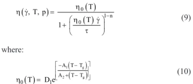
p 0= along the front flow (8) According to Guerrier et al.[21], the cross viscosity model
is directly related to temperature and pressure dependence variables:
(
)
( )
( )
0 1 n 0 T , T, p T 1 − η η γ = η γ + τ (9) where:( )
( ) ( ) 1 g 2 g A T T A T T 0 T D e1 − − + − η = (10)where D1 is the viscosity at a reference temperature
(1.92686 e16 Pa.s); 2
D = 236.15K; Tg is the glass transition
temperature of the polymer (108 °C); and the other constants are A1= 34.52, A2= 51.6K, τ = 63,836 Pa, and n = 0.19118.
2.3.2 Cooling simulation
Only after the mold cavity fill phase does Solidworks Plastics perform the simulations of the mold cooling
and solidification phase. The governing equation for the mid-plane cooling stage is the average steady-state cycle temperature governed by a second-order partial differential equation, the Laplace equation:
2 2 2 2 T 0T x y ∂ + ∂ = ∂ ∂ (11)
where T is the average cycle temperature. This equation can be solved with the appropriate boundary conditions imposed on the different mold boundaries, i.e., the cavity surface, cooling channel surface, and external surface[17]. Transient
heat conduction gives the field temperature in the mold as:
2 2 m m m m T2 T2 m m T k C t x y ∂ ∂ ∂ = + = ρ ∂ ∂ ∂ (12)
where TM is the mold temperature; kM is the thermal conductivity of the mold; ρm is the density of the mold; and
CM is the specific heat of the mold. 2.4 Simulation validation
To validate the simulations, a qualitative and quantitative comparison of the lid injection process was performed. The cover design was built in SolidWorks with the same
proportions as the actual part. Additionally, the same “U” cooling channels were reproduced in the simulations for validation, as shown in Figure 5.
Figure 5. Validation simulation performed on the cover with a “U” type cooling channel.
For this type of validation, the simulation processing parameters must be equal to the experimental conditions. The processing parameters of this validation are represented in Table 1.
In Table 1, P0 is the injection pressure, T0 is the injection temperature, and TL is the water temperature in the feed channels. For each condition in Table 1, ten experimental samples were performed to qualitatively and quantitatively validate the simulations.
2.5 Mold cooling system modifications
With the validation of the simulations performed, new cooling channels were developed in CAD to analyze which geometry will provide a faster homogeneous solidification. The geometries chosen for the cooling channels were the “Z”, “Rectangular”, and “Helical” geometries. A representation of these geometries can be seen in Figure 6.
The simulations were performed considering three different types of cooling channels to compare which one is more efficient, including the “U” channel itself. However, to make such modifications to the actual mold, it was necessary to modify the existing mold, which takes time and cost.
2.6 Cost analysis for modifications
With the simulation results, as there is the possibility of improving the solidification efficiency, a payback analysis was performed to verify if the modification investment is viable for the company. This type of analysis can ratify the amount of time that the amount invested can be repaid and/or depreciated during the assessed period[22,23].
2.6.1 Taxed revenue
Taxed revenue (TR) is the calculated revenue value, which is added to the tax amounts inherent to the area of interest:
(
)
TR= GR RV d+ − (13)
where GR is gross revenue; RV is the residual value; and d is the depreciation rate.
2.6.2 Payback (Pb)
To obtain the payback of the invested capital, use:
(
)
Inv MRA Log 1 AS Pb Log 1 MRA − − = + (14)where Pb is the payback; Inv is the value of the investment;
MRA is the minimum rate of attractiveness; and AS is the
annual savings. 2.6.3 Net present value
For calculating the net present value (NPV), the following equation is used:
(
)
(
)
n j n j j 0 j 0 NPV Rj 1 i− Cj 1 i− = = =∑ + −∑ + (15) 2.6.4 Depreciation (d)To calculate how much the project will depreciate annually, use the equation:
(
Inv RV)
d t −
= (16)
where d is the depreciation rate and t is the useful life of the investment. The calculations were performed considering the three different proposed and simulated modifications.
3. Results and Discussions
This stage presents the results obtained experimentally and by simulation. Based on these results, a case study was elaborated, verifying the obtained quality and the economic viability of altering the original mold cooling circuit.
3.1 Validation I: qualitative analysis
With the intent to apply a qualitative analysis of the cap injection mold, ten samples were run on the injection molding machine using the processing parameters in Table 1. The qualitative comparison of this process can be compared with simulations performed under the same processing conditions, as shown in Figure 7.
Figure 6. Proposed modifications to the lid mold cooling system. (a) “Z” type circuit; (b) “Rectangle” type circuit; (c) “Helical” type circuit. Table 1. Processing parameters for simulation validation.
Step P0 (bar) T0 (°C) TL (°C) a 30 210 35 b 50 210 35 c 60 210 35 d 70 210 35 e 85 210 35 f 95 210 35
According to the results, coherence is verified since the results found experimentally are similar to the value obtained in the simulation, as shown in Figure 7. Visually, it is possible to observe the similarity between the processes. Figure 7f illustrates the cap with 100% of its filled volume, so 9.5MPa (95bar) filler pressure is required. The fully filled lid has a volume of 15.52 cm3 and a mass of 14 grams. To verify the
filling pressure phases, Figure 7a demonstrates the step with only 3MPa (30bar). This pressure allows the injection of only 4.9 cm3, which represents 31.57% of the total volume. Only
4.42 grams of plastic material is inserted into the cavity.
3.2 Validation II: quantitative analysis
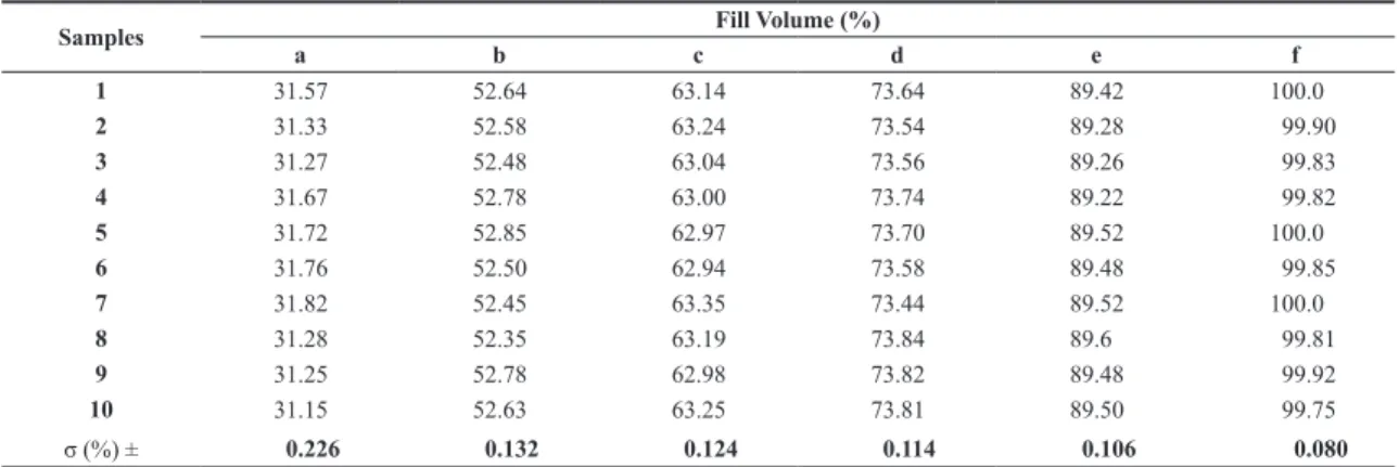
With the ten samples, it is possible to verify the variability presented between them, as shown in Table 2, and also becomes possible to calculate the standard deviation [σ (%)] among them resulting from the referred samples.
The samples have a proportional standard deviation; that is, the more filled the cavity is, the smaller its standard deviation due to the better stability provided by increased the part filling pressure. After performing the experiments and simulations, some parameters can be compared to validate the simulations quantitatively.
Simulations provide the parameters, which can also be collected experimentally, in a general analysis of results. These parameters can be observed in Table 3.
Consistency between the results of experimental fill volume (Fv) and simulated fill volume (Fvs) is verified since they have the same tendency and proportionality of fill. As the injection pressure is gradually increased at the rate of fill, the volume cavity behaves evenly. The values of Fvs are incremented every five %. That is, there is no decimal precision in the simulated results, which means the filled volume values had little difference between the experimental and the simulated ones.
Figure 7. Qualitative validation under process conditions: (a) step a; (b) step b; (c) step c; (d) step d; (e) step e; (f) step f. Table 2. The filling volume of the samples and the corresponding standard deviation.
Samples a b cFill Volume (%)d e f
1 31.57 52.64 63.14 73.64 89.42 100.0 2 31.33 52.58 63.24 73.54 89.28 99.90 3 31.27 52.48 63.04 73.56 89.26 99.83 4 31.67 52.78 63.00 73.74 89.22 99.82 5 31.72 52.85 62.97 73.70 89.52 100.0 6 31.76 52.50 62.94 73.58 89.48 99.85 7 31.82 52.45 63.35 73.44 89.52 100.0 8 31.28 52.35 63.19 73.84 89.6 99.81 9 31.25 52.78 62.98 73.82 89.48 99.92 10 31.15 52.63 63.25 73.81 89.50 99.75 σ (%) ± 0.226 0.132 0.124 0.114 0.106 0.080
Table 3. Qualitative validation under process conditions: (a) step a; (b) step b; (c) step c; (d) step d; (e) step e; (f) step f.
Step Fv (%) σ (%) Fvs (%) Eft (s) tps (s) Sft (s) trs (s) Efct (ºC) Sfct (°C)
a 31.57 ± 0.226 35.0 0.70 0.47 3.0 3.04 90.55 92.09 b 52.64 ± 0.132 55.0 1.20 1.09 5.0 5.12 93.75 95.74 c 63.14 ± 0.124 65.0 1.30 1.18 6.5 6.91 96.55 98.45 d 73.64 ± 0.114 75.0 1.60 1.48 7.5 7.74 97.70 99.40 e 89.42 ± 0.106 90.0 1.75 1.63 8.0 8.09 98.62 100.14 f 100.0 ± 0.080 100.0 1.90 1.79 9.5 9.67 99.80 101.68
The experimental fill time (Eft), and simulated fill time (Sft) follow the same trend, which is proportional to volume. The time increases when the injection pressure value is high. The results of tpe and tps present similar values, demonstrating their consistency. Regarding the experimental final cooling temperature (Efct) and simulated cooling final temperature (Sfct), the obtained values also show cohesion since the rates of increase are linear. The temperature of the part rises in proportion to the increase in the filled volume of the cavity, i.e. the more material is injected into the mold cavity, the higher the temperature of the mold cavity.
3.3 Analysis of modifications with alternative cooling systems
After validating the parameters and results, the solidification efficiencies and cost-effectiveness of various injection mold cooling systems were verified using SolidWorks Plastics.
3.3.1 Cooling time
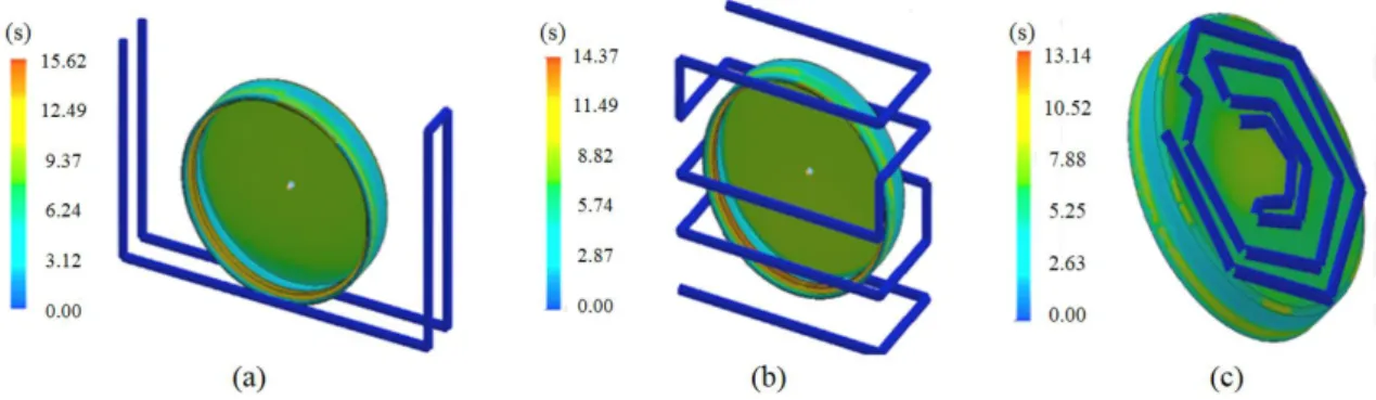
More excellent reliability of the values obtained for cooling is set in the software to ensure some parameters for all simulation steps, such as coolant temperature (water) at 30 °C and maximum melting temperature of polymer material at 210 °C. The maximum cooling time values obtained by the simulation ranged from 13.15 to 15.9 s for the helical and “U” type circuits, respectively, as can be seen in Figure 8.
Figure 8 shows the results obtained from simulations in which it is possible to verify coherence between the value obtained in the simulation of the “U” circuit, original mold, and the value obtained in the injection molding process standard sheet, 15.69 and 16 seconds respectively. Additionally, the most efficient cooling system is helical since it required a shorter cooling cycle time for solidifying the injected part, dramatically reducing the cycle time.
As shown in Figure 8, the system that presented the least efficient result was the “U” type system, followed by the “Z”, rectangular, and finally, the one that presented the best result, helical.
3.3.2 Part temperature after solidification
The results obtained from the simulation software for the lid temperature after the cooling step ranged from 101.68 to 93.66 °C for the “U” and helical circuits, respectively, as shown in Figure 9.
Figure 9 shows the results obtained in the simulation. These results verify coherence between the value obtained in the simulation of the original “U” circuit of the mold and the value obtained by a laser thermometer, 101.68 and 99.8 °C, respectively.
The most efficient cooling system is the coil, because it obtained a higher heat exchange rate between the injected mass and the cooling system refrigerant, requiring less cooling time to reduce the lid temperature inside the mold, causing cycle loss and increasing productivity.
3.3.3 Mold temperature after cooling
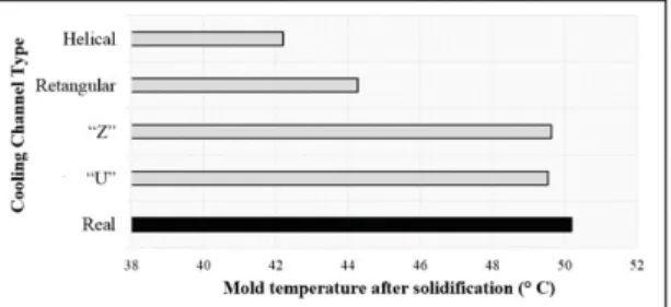
The results obtained by the simulation software of the mold temperature after the cooling step varied between 49.54 and 42.2 °C for the “U” and helical circuits, respectively, as shown in Figure 10.
Figure 10 shows the results obtained in simulation, proving that the most efficient cooling system is the helical one, since it obtained a higher heat exchange rate between the injected mass and the cooling system refrigerant, maintaining a lower temperature than the injection mold. The more stable and closer to the coolant temperature, the better the quality of the injected product will be and the less time the machine will need to cool down.
3.4 Payback analysis in constructing cooling systems
The results found during the simulation stages showed that the helical cooling circuit presented higher efficiency because it required a shorter cooling time for the part. The manufacturing costs of a new injection mold cavity cooling system were evaluated by checking the system cost and payback.
With the original “U” type mold cooling system, the total injection cycle is 22s. As the mold under study was composed of 8 productive cavities, every 22s, lids are produced. 1,300 caps are produced per hour, and the machine works 24 hours a day, so 31,200 units are produced per day. Monthly, the machine works, on average, 17 days with the lid mold. Due to the high contingent of molds, there is a need to produce other products in the same injector. Adding maintenance stops and color changes, the average monthly
Figure 8. Cooling time variation.
Figure 9. Cover temperature after solidification in each type of cooling system.
Figure 10. Mold temperature after solidification in each type of cooling system.
production is 487,500 caps (375h). It is possible to make 5,600,000 lids annually, according to Table 4.
Changing the mold cooling circuit to type “Z” increases production by 24,000 pieces per year. Production capacity increases with the rectangular circuit, allowing the production of 310,000 more lids compared to the original system (“U”). The system that showed the highest efficiency is the helical type, where the simulation results showed that it is possible to reduce the cooling time by 2.5s, i.e., the injection cycle can be obtained with 19.5s. It would be possible to produce 1,475 pieces per hour, 35,400 injected caps per day, or 553,000 per month. 6,200,000 lids could be made annually. Changing the cooling system increases 600,000 caps over a year.
Comparing the most effective (helical) and second (rectangular) systems, the annual increase in production practically doubles, 600,000 and 310,000, respectively; that is, the helical circuit is the most efficient. The market value of the cap is $0.12. Annual expenses for electric power, machine maintenance, and molds are R$250,000.00.
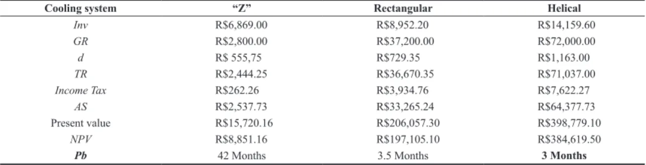
According to the data shown in Table 5, the helical system is the one that demands the highest investment value. However, due to its efficiency, as demonstrated in the simulation stages, the return on invested capital comes in less time compared to other circuits. The helical system becomes more attractive due to the year-end gross revenue. It is directly related to improved mold cooling efficiency and reduced injection machine cycle time.
Given the data obtained and elaborate calculations, the helical cooling system is the most attractive because the return on investment occurs in less time compared to the “Z” and rectangular systems.
4. Conclusions
The simulations carried out make it possible to analyze the efficiency of the solidification steps for different thermoplastic injection mold cooling systems, demonstrating
that the helical geometry cooling system is more efficient. The remarkable points are:
1. The simulations were validated with experimental tests showing the accuracy of the simulations of the new cooling system;
2. With the validation, it was possible to numerically simulate different cooling channel geometries for the lid injection mold, to compare the different modifications proposed;
3. Calculations of return on invested capital demonstrated that the helical circuit obtained better performance, both in terms of efficiency and product quality, as well as in the shorter return time of the invested value; 4. Given this, it is highly recommended to change the
injection mold cooling design. With the change, it is possible to increase productivity and product quality. This demonstrates greater precision in decision making for changes and modifications of new designs; 5. The results showed that numerical simulation is a
practical tool for engineers and designers to justify future maintenance or modifications to the injection molds already existing within the company.
5. Acknowledgements
The authors gratefully acknowledge CAPES (Coordination for the Improvement of Higher Education Personnel, Brazil) for financial support.
6. References
1. Alfrey, T., & Gurnee, E. (1971). Polímeros orgânicos: série de
textos básicos de ciência dos materiais. São Paulo: Blucher.
2. Mercado-Colmenero, J. M., Rubio-Paramio, M. A., Marquez-Sevillano, J. J., & Martin-Doñate, C. (2018). A new method for the automated design of cooling systems in injection molds. Table 4. Estimated production for each cooling system.
Cooling system Cooling Time (s) Total cycle (s) Quantity of Parts/h Quantity of Parts/day Parts/MonthQuantity of Quantity of Parts/Year
“U” 15.7 22.0 1,300 31,200 487,500 5,600,000
“Z” 15.6 21.9 1,315 31,560 493,000 5,624,000
Retangular 14.4 20.7 1,390 33,360 521,250 5,910,000
Helical 13.2 19.5 1,475 35,400 553,000 6,200,000
Table 5. Results of values for payback calculations.
Cooling system “Z” Rectangular Helical
Inv R$6,869.00 R$8,952.20 R$14,159.60 GR R$2,800.00 R$37,200.00 R$72,000.00 d R$ 555,75 R$729.35 R$1,163.00 TR R$2,444.25 R$36,670.35 R$71,037.00 Income Tax R$262.26 R$3,934.76 R$7,622.27 AS R$2,537.73 R$33,265.24 R$64,377.73 Present value R$15,720.16 R$206,057.30 R$398,779.10 NPV R$8,851.16 R$197,105.10 R$384,619.50
Computer Aided Design, 104, 60-86. http://dx.doi.org/10.1016/j.
cad.2018.06.001.
3. Clemente, M. R., & Panão, M. R. O. (2018). Introducing flow architecture in the design and optimization of mold inserts cooling systems. International Journal of Thermal Sciences, 127, 288-293. http://dx.doi.org/10.1016/j.ijthermalsci.2018.01.035. 4. Jahan, S. A., Wu, T., Zhang, Y., Zhang, J., Tovar, A., &
Elmounayri, H. (2017). Thermo-mechanical design optimization of conformal cooling channels using design of experiments approach. Procedia Manufacturing, 10, 898-911. http://dx.doi. org/10.1016/j.promfg.2017.07.078.
5. Corazza, E. J., Sacchelli, C. M., & Marangoni, C. (2012). Cycle time reduction of thermoplastic injection using nitriding treatment surface molds. Información Tecnológica, 23(3), 51-58. http://dx.doi.org/10.4067/S0718-07642012000300007. 6. Hassan, H., Regnier, N., Arquis, E., & Defaye, G. (2016).
Effect of cooling channels position on the shrinkage of plastic material during injection molding. In Proceedings of the 19th French Congress on Mechanics (pp. 1-6). Marseille: French
Association of Mechanics.
7. Blass, A. (1988). Processamento de polímeros (2. ed.). Florianópolis: Editora UFSC.
8. Oliaei, E., Heidari, B. S., Davachi, S. M., Bahrami, M., Davoodi, S., Hejazi, I., & Seyfi, J. (2016). Warpage and shrinkage optimization of injection-molded plastic spoon parts for biodegradable polymers using Taguchi, ANOVA and artificial neural network methods. Journal of Materials Science
and Technology, 32(8), 710-720. http://dx.doi.org/10.1016/j.
jmst.2016.05.010.
9. Steinko, W. (2004). Avaliação do projeto térmico do molde garante qualidade e redução de custos. Plástico Industrial,
6(1), 64-71.
10. Park, H. S., & Dang, X. P. (2017). Development of a smart plastic injection mold with conformal cooling channels.
Procedia Manufacturing, 10, 48-59. http://dx.doi.org/10.1016/j.
promfg.2017.07.020.
11. Xiao, C. L., Huang, H. X., & Yang, X. (2016). Development and application of rapid thermal cycling molding with electric heating for improving surface quality of microcellular injection molded parts. Applied Thermal Engineering, 100(1), 478-489. http://dx.doi.org/10.1016/j.applthermaleng.2016.02.045. 12. Wang, W., Zhang, Y., Li, Y., Han, H., & Li, B. (2018). Numerical
study on fully-developed turbulent flow and heat transfer in inward corrugated tubes with double-objective optimization.
International Journal of Heat and Mass Transfer, 120(1),
782-792. http://dx.doi.org/10.1016/j.ijheatmasstransfer.2017.12.079. 13. Vieira, R. P., & Lona, L. M. F. (2016). Simulation of temperature
effect on the structure control of polystyrene obtained by atom transfer radical polymerization. Polímeros: Ciência e Tecnologia,
26(4), 313-319. http://dx.doi.org/10.1590/0104-1428.2376.
14. Kantor, N. L. S. (2011). Análise da viabilidade técnica e
econômica da automação de um armazém de grãos. In Anais do
13º Congresso Nacional de Estudantes de Engenharia Mecânica
(pp. 1-2). Erechim: Associação Brasileira de Engenharia e Ciências Mecânicas.
15. Domingos, B. S., Moreira, C. R., Resende, E. W. B. S., Moreira, C. R., Resende, E. W., Rodrigues, D. M. S., & Dornelas, J. O. (2017). Estudo de payback simples para a substituição do gás
liquefeito de petróleo pelo biogás em uma unidade hospitalar em Minas Gerais. In Anais do 9º Simpósio de Engenharia de Produção de Sergipe (pp. 193-204). São Cristóvão: Departamento
de Engenharia de Produção, Universidade Federal de Sergipe. 16. Mendes, E. C., & Miranda, D. A. (2018). Análise de payback
aplicado no processo de automatização de podas na produção de Buxus. In Anais do 3º Congresso Nacional de Inovação e Tecnologia (pp. 1-10). São Bento do Sul: INOVA.
17. Miranda, D. A., & Nogueira, A. L. (2019). Simulation of an injection process using a CAE tool: assessment of Operational conditions and mold design on the process efficiency. Materials
Research, 22(2), e20180564.
http://dx.doi.org/10.1590/1980-5373-mr-2018-0564.
18. Sacchelli, C. M., Miranda, D. A., Drechsler, M., & Nogueira, A. L. (2017). Simulação computacional da injeção de termoplásticos:
comparação de ferramentas tipo CAE. In Anais do 9º Congresso Brasileiro de Engenharia de Fabricação. Joinville: COBEF.
http://dx.doi.org/10.26678/ABCM.COBEF2017.COF2017-1320.
19. Miranda, D. A., & Nogueira, A. L. (2017). Influência dos
parâmetros de processo e da presença de saídas de gases na eficiência de moldes de injeção de peças em poliestireno cristal.
In Anais do 14º Congresso Brasileiro de Polímeros (pp. 1-5). Águas de Lindóia: Associação Brasileira de Polímeros. 20. Fernandes, C., Pontes, A. J., Viana, J. C., & Gaspar-Cunha, A.
(2016). Modeling and optimization of the injection-molding process: a review. Advances in Polymer Technology, 17(2), 429-449. http://dx.doi.org/10.1002/adv.21683.
21. Guerrier, P., Tosello, G., & Hattel, J. H. (2017). Flow visualization and simulation of the filling process during injection molding.
CIRP Journal of Manufacturing Science and Technology, 16(1),
12-20. http://dx.doi.org/10.1016/j.cirpj.2016.08.002. 22. Hummel, P. V. R., & Taschner, M. R. B. (1995). Análise e
decisão sobre investimentos e financiamentos: engenharia econômica: teoria e prática (4. ed.). São Paulo: Atlas.
23. Miranda, D. A., & Cristofolini, R. (2016). Análise de retorno
financeiro aplicado a dois robôs autonômos manipuladores que atuam na descarga de peças no processo de injeção de termoplásticos. In Anais do 6º Congresso Brasileiro de Engenharia de Produção (pp. 1-12). Ponta Grossa: Associação
Paranaense de Engenharia de Produção.
Received: Oct. 01, 2019 Revised: Mar. 27, 2020 Accepted: Apr. 13, 2020