ISSN 0001-3765 www.scielo.br/aabc
Large amplitude oscillations for a class of symmetric polynomial differential systems in R3
JAUME LLIBRE1 and MARCELO MESSIAS2
1Departament de Matemàtiques, Universitat Autónoma de Barcelona, 08193 Bellaterra, Barcelona, Catalonia, Spain 2Departamento de Matemática, Estatística e Computação, Faculdade de Ciências e Tecnologia da UNESP
Caixa Postal 467, 19060-900 Presidente Prudente, SP, Brazil
Manuscript received on January 17, 2007; accepted for publication on September 27, 2007; presented byMANFREDO DOCARMO
ABSTRACT
In this paper we study a class of symmetric polynomial differential systems inR3, which has a set of parallel
invariant straight lines, forming degenerate heteroclinic cycles, which have their two singular endpoints at infinity. The global study near infinity is performed using the Poincaré compactification. We prove that for alln∈Nthere isεn>0 such that for 0< ε < εnthe system has at leastnlarge amplitude periodic orbits bifurcating from the heteroclinic loop formed by the two invariant straight lines closest to thex-axis, one
contained in the half-spacey>0 and the other iny<0.
Key words:infinite heteroclinic loops, periodic orbits, symmetric systems.
1 INTRODUCTION
In this paper we study the following class of symmetric polynomial differential systems inR3
˙
x = d x
dt = y,
˙
y = d y
dt = z, (1)
˙
z = d z
dt = p(y)+ε q(x)z, whereεis a small positive real parameter,
p(y) =
m
i=0
aiyi and q(x) = m/2
i=1
b2i−1x2i−1, (2)
AMS Classification: Primary: 58F21; Secondary: 34C05, 58F14. Correspondence to: Marcelo Messias
withman even natural number,a0>0 andbm−1>0. Under these assumptions system (1) has no singular points in R3. This system can be extended to an analytic system on a closed ball of radius one, whose interior is diffeomorphic toR3and its boundary (a 2-dimensional sphereS2) plays the role of infinity. The technique for making such an extension is called the Poincaré compactification, which is described in detail in Appendix 1.
We suppose that the polynomial p(y)which appears in the third equation of system (1) has k ≥ 2
simple real rootsri,i =1, . . . ,k, with at least two of them having opposite signs. In this way the system hask parallel invariant straight lines given by
γi =
γi(t) = (x(t),y(t),z(t)) = (rit,ri,0)∈R3: t∈R
.
These invariant straight lines tend toward two diametrally opposite singular points at infinity whent → ±∞, corresponding to the endpoints of thex-axis, after the Poincaré compactification. In fact, each straight lineγi reaches the points at infinity with sloperi in a sense that we shall describe in the Subsection 2.2. Considerr1andr2the real roots of p(y), withr1the largest negative andr2the smallest positive root. In this way, the invariant linesγ1=(r1t,r1,0): t∈Randγ2=r2t,r2,0): t∈Rtogether with the two singular points at infinity located at the end of thex-axis form a degenerate heteroclinic loopL.
It is important to observe that system (1) is invariant under the symmetry
S: (x,y,z,t)→(−x,y,−z,−t).
This means that ifγ (t)=(x(t),y(t),z(t))is a solution of the system, then
Sγ (t) = −x(−t),y(−t),−z(−t)
is a solution too. So, due to the symmetry, ifγ has a point on they-axis, then the orbitsγ and its symmetric orbitS(γ )with respect to the y-axis coincide. Moreover ifγ has two points on the y-axis, thenγ (t)is a
symmetric periodic orbit. Therefore a way to find periodic orbits is to look for orbits having two points
on the y-axis. This technique will be used here to prove the existence of large amplitude periodic orbits bifurcating from the loopL described above.
Letδ >0 but small. We take an open segmentŴ= {(0,y,0):r1<y < δ+r1}(note thatr1<0) of they-axis with its left endpoint(0,r1,0)on the heteroclinic loop L =γ1∪γ2and we will follow its image under the flow of system (1) until its first intersection with the planex =0 near the point(0,r2,0)ofL, see Figure 4. We denote byπ the Poincaré map going fromx =0 near(0,r1,0)tox =0 near the point
(0,r2,0). Then we shall prove thatπ(Ŵ)is a spiral near the point(0,r2,0)giving finitely many turns for everyε > 0 sufficiently small. This number of turns tends to infinity asε → 0. The orbits through the
intersection points ofπ(Ŵ)with they-axis are periodic because, by construction, they have two points on they-axis. Using these ideas in Section 2 we shall prove the following result. As usual we denote byNthe set of positive integers.
THEOREM1. For alln ∈ Nthere isεn > 0such that system (1) forε ∈ (0, εn)has at leastn periodic
The idea that heteroclinic loops to infinity can create a set of large amplitude periodic orbits (and even chaotic ones) has already appeared in several papers, see for instance (Newell et al. 1988).
Llibre, MacKay and Rodríguez (Llibre et al. 2004, preprint) study system (1) for the case where considering p(y)=1−y2andq(x)=x. In this case the system is equivalent, by a change of coordinates and a reparametrization of time, to the differential equation
y′′′+y′′y+λ1−y′2=0, (3)
which is related to boundary layer theory in fluid mechanics where it is know as the Falkner-Skan equation (see Guyon et al. 1991) for a derivation of this equation. See also (Sparrow and Swinnerton-Dyer 1995, 2002) for analytical information on the existence of periodic and other types of orbits in the Falkner-Skan equation. In fact, for this system, there is a hyperbolic subshift near the infinite heteroclinic loop (Llibre et al. 2004, preprint). But, in this paper, we will restrict attention to finding large amplitude periodic orbits and understanding the geometrical mechanism which create them.
2 PROOF OF THE THEOREM 1
In this section we shall prove our main result. The proof is constructive and will be presented in the four next subsections. In order to fix the notation we write the polynomial differential system (1) inR3in the form
˙
x = P1(x,y,z) = y,
˙
y = P2(x,y,z) = z,
˙
z = P3(x,y,z) = p(y)+εq(x)z,
where p(y)andq(x)are given in (2) andε >0 is a small parameter. In what follows we denote by X the vector field associated to this system.
2.1 THE HETEROCLINIC LOOP L
Letγ1(t)=(r1t,r1,0)andγ2(t) =(r2t,r2,0)be the two invariant straight lines of system (1), related to the largest negative and the smallest positive real root of p(y),r1andr2, respectively. The endpoints of these two lines at infinity in the Poincaré compactification are the origins p1=(0,0,0)andp2=(0,0,0) of the local chartsV1andU1, respectively. For more details see Appendix 1.
2.2 THE LOCAL FLOW AT THE SINGULAR POINT p1AT INFINITY
Using the results stated in Appendix 1, we have that the expression of the Poincaré compactification p(X) in the local chartV1is
˙
z1 = z21z3m−1−z2zm3−1,
˙
z2 = z1z2zm3−1−p(z1,z3)−ε z2
z3 q(z3), (4)
˙
where
p(z1,z3) =
m
i=0
ai zi1 zm3−i and q(z3) = m/2
i=1
b2i−1zm3−(2i−1). (5)
We want to study the local flow of this system around the singular point p1 = (0,0,0). The eigenvalues of the linear part of this flow at p1 = (0,0,0)are 0, 0 and−εbm−1. As we are consideringbm−1 > 0, the singular point p1 has a two dimensional central manifold and the flow outside this manifold tends exponentially to it because of the negative eigenvalue−εbm−1. Now we shall study the flow on this central
manifold. For more details on central manifolds see (Carr 1981, Chow and Hale 1982).
PROPOSITION 2. The invariant straight lines γi in a neighborhood of p1 are contained in the central
manifold of the singular point p1of system (4).
PROOF. From Theorem 1 of (Carr 1981, page 4), we know that there exists a center manifold to p1given byz2=h(z1,z3)in a neighborhood of p1, which satisfies the conditions
h(0,0) = Dh(0,0)=0 and z2˙ = d
dth(z1,z3) = ∂h ∂z1z1˙ +
∂h
∂z3z3˙ (6) (for more details see (Carr 1981, page 5)). Moreover, the flow on this center manifold is governed by the 2-dimensional system
˙
z1 = z21zm3−1−zm3−1h(z1,z3),
˙
z3 = z1zm3. (7) Note that the straight linez3=0 is filled of singular points.
Considering conditions (6) and the derivatives given in system (4), the function h must satisfy the equation
z21zm3−1−h zm3−1 ∂h ∂z1 +z1z
m 3
∂h ∂z3 −
z1zm3−1h− p−ε h z3 q(z3)
=0,
or, equivalently,
zm3−1
z21∂h ∂z1 −h
∂h
∂z1+z1z3 ∂h ∂z3 −hz1
+p+ε h
z3 q(z3)=0.
Expanding the functionh(z1,z3)in power series in a neighborhood of p1, and substituting it in the previous equation we obtain
h(z1,z3)= − 1
εbm−1 p
(z1,z3)+Om+1(z1,z3), (8)
where p(z1,z3)is given in (5). Since system (1) has the invariant straight lines x = r t, y = r,z = 0,
wherer is a real root of the polynomialp(y)given in (2), it follows that system (4) has the invariant straight linesz1 =r z3,z2 =0 (observe that we take x = 1/z3, y =z1/z3andz = z2/z3in the local chartV1in the compactification procedure, see Appendix 1). Therefore, system (7) has also the invariant straight lines z1=r z3. So for system (7) we have that
˙
z1−rz3˙
z1=r z3 = −z
m−1
3 h(r z3,z3)=0.
Recall thatr1 andr2 denote the real roots of p(y), withr1 the largest negative andr2 the smallest positive. Such a roots exist by assumptions. We denote by γ1 and γ2 the two invariant straight lines associated to these two roots, respectively.
PROPOSITION3. On the center manifold of the singular point p1of system (4) and in a neighborhood of
p1restricted toz3 <0, there exists a hyperbolic sector having as separatrices the invariant straight lines
γ1andγ2restricted to this neighborhood.
PROOF. Again we use the notations introduced in the proof of Proposition 2. We consider now the invariant straight linesγ (t)=(r t,r,0)withr a real root of the polynomial p(y).
Suppose thatr <0, then on the straight lineγ and on the half-planex <0; i.e. on the half-straight line γ contained inV1, considering the change of coordinates in the compactification process (see Appendix 1 for details) we have thatz3 =1/x <0,z1= y/x >0,z1˙ <0 (recall that on these invariant straight lines h(z1,z3)=0) andz3˙ >0.
Similarly for the straight lineγ withr >0 contained inV1, we have thatz3=1/x <0,z1= y/x <0,
˙
z1<0 and˙z3<0.
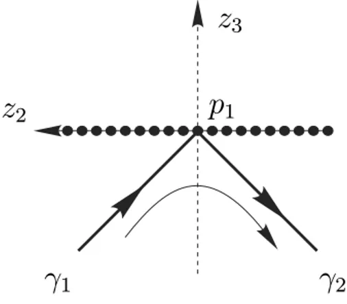
In short the flow on the straight linesγ1andγ2in a neighborhood of p1is as it is described in Figure 1.
z
2z
3p
1γ
1γ
2Fig. 1 – The flow on the center manifold.
Using (8) the differential system (7) on the central manifoldz2=h(z1,z3)of the singular pointp1for system (4) can be written, after a rescaling of the time byzm3−1, as
˙
z1= z21+ 1
εbm−1 p
(z1,z3)+Om+1(z1,z3),
˙
z3= z1z3.
(9)
We claim that the unique directions for tending to the origin of system (9) when the timet → ±∞are the ones given by the invariant straight linesz1=r z3withr a real root of the polynomialp(y). Before proving the claim we end the proof of the proposition.
defined byγ2starts atp1. By the claim there are no other directions between the directions given byγ1and γ2for reaching the singular point p1in forward or backward time. Now from the differential system (7) on the central manifoldz2 =h(z1,z3)of the singular point p1and taking into account (8) we have that
˙
z1
z1=0 = a0 εbm−1
z23m−1 + O(z23m).
Onz3<0 this expression is negative, so we have a hyperbolic sector. Recall that it is known that the local phase portraits of the singular point p1is a finite union of hyperbolic, elliptic and parabolic sectors (see, for instance, Andronov et al. 1973 or Dumortier et al. 2006).
Now we prove the claim. First we write system (9) in polar coordinates(ρ, θ )given byz1 =ρcosθ andz3=ρsinθ. The system becomes
˙
ρ = cosθ ρ2+aρmp(cosθ,sinθ )+O(ρm+1),
˙
θ = −asinθp(cosθ,sinθ )ρm−1+O(ρm),
(10)
wherea = a0/(εbm−1). If a solution(ρ(t), θ (t))of this system tends to the origin whent → ±∞(i.e. ρ(t)→0 whent → ±∞), then the limit ofθ (t)whent → ±∞exists, because the solution(ρ(t), θ (t)) cannot spirals tending to the origin due to the existence of invariant straight lines through the origin.
Now from the differential system (10) it is clear that the unique directions θ∗ in which a solution (ρ(t), θ (t))can reach the origin whent → ±∞are the zeros of sinθp(cosθ,sinθ ). That is, the directions of the invariant straight linesz1 =r z3withr a real root of the polynomial p(y), andz3 =0. Hence the
claim is proved. Consequently Proposition 3 follows.
2.3 HAMILTONIAN STRUCTURE ASSOCIATED TO SYSTEM(1)WITHε=0
In this Subsection we analyze the flow of system (1) forε = 0 in the(y,z)-plane. The equations for y˙
andz˙of system (1) withε =0 are the equations of the following Hamiltonian system with one degree of
freedom
˙
y = d y
dt =z,
˙
z = d z
dt = p(y),
(11)
with Hamiltonian given by
H(y,z) = 1
2z 2
−
p(y)d y = 1
2z 2
−
m
i=0 ai
(i+1)y
i+1 .
Under the assumptions on the polynomial p(y), this Hamiltonian system hask ≥2 singular points, given
by(ri,0), where theri’s are the real roots of p(y). The jacobian matrix of system (11) calculated at one of these singular points is given by
D X(ri,0) =
0 1 p′(ri) 0
;
Since p(r1) = 0, r1 being the largest negative root of p(y) and p(0) = a0 > 0, it follows that p′(r1)≥0. We suppose that p′(r1) >0, and in a similar way we also assume that p′(r2) <0, wherer2is the smallest positive root of p(y). Therefore,(r1,0)is a saddle and(r2,0)is a center.
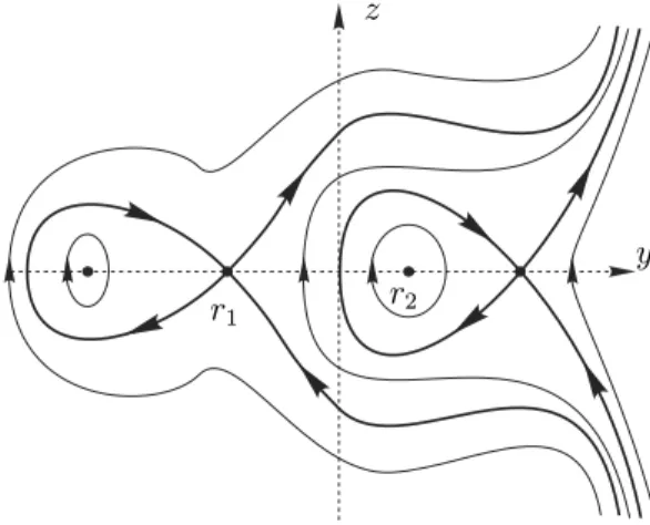
If all the real roots of p(y)are simple, then the singular points(ri,0)alternate between saddles and centers. In Figure 2, a possible phase portrait for the Hamiltonian system (11) is shown for the particular case in which the number of real roots of p(y)isk =4 (see Example 4 below).
z
y
r1 r
2
Fig. 2 – The orthogonal projection of the flow of system (1) withε=0 into the(y,z)–plane.
From Figure 2 it is easy to understand the flow of system (1) whenε=0. The singular points of Figure
2 correspond to the invariant straight linesγi; i.e. the point(ri,0)is the orthogonal projection with respect to thex-axis ofγi onto the(y,z)-plane. Observe that the invariant lines closest to thez-axis areγ1andγ2. We note that the flow of system (1), near the invariant straight line γ2 when ε = 0, is surrounded by invariant cylinders, the flow on these cylinders goes from −∞ to +∞ in the x variable increasing monotonically becausex˙ = y > 0 in a neighborhood ofγ2. Hence, the flow of system (1) whenε = 0
sufficiently near toγ2rotates around this straight line. Let
h2 = H(r2,0) =
m
i=0 ai
(i+1)r
i+1 2 .
Then for the periodic orbits of the Hamiltonian system (11) surrounding the center(r2,0)the Hamiltonian H takes values in an open interval with endpointh2. LetT(h)be the period of the periodic orbit of this center contained inH =h. We introduce thepotential energy
U(y) = −
p(y)d y = −
m
i=0 ai
(i+1)y
i+1 ,
associated to the Hamiltonian system (11). Then, from (Arnold 1980, page 20) we know that
lim h→h2
T(h) = 2π
U′′(r2) =
2π
β , (12)
where
β = −
m
i=1
Therefore the periods of the periodic orbits close to the point(r2,0)are finite. This result will be used in the proof of Theorem 1 in the next Subsection.
EXAMPLE4. If we take p(y)=y4−5y2+4 and q(x)=x +x3, then system(1)has the form
˙
x = y,
˙
y = z, (13)
˙
z = y4−5y2+4+ε z(x+x3).
The polynomialp(y)has the four simple real roots: −2,−1, 1, 2. So this system has four invariant straight
lines and forε=0 the orthogonal projection with respect to thex-axis of its solutions on the(y,z)-plane is shown in Figure 2.
The expression of the Poincaré compactification of(13)in the local chartV1is
˙
z1 = z21z33−z2z33,
˙
z2 = z1z2z33−
4z4
3−5z21z23+z41
−ε z2
z23+1
, (14)
˙
z3 = z1z33.
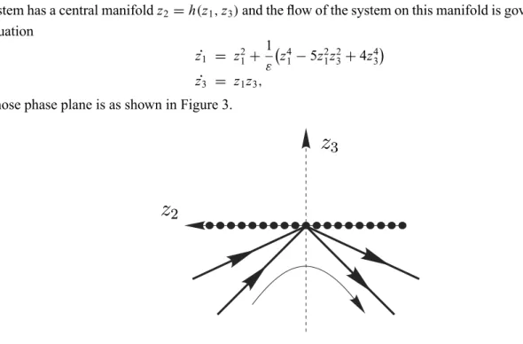
The origin p1 = (0,0,0)is a singular point of this vector field with eigenvalues 0,0,−ε, and then the system has a central manifoldz2 =h(z1,z3)and the flow of the system on this manifold is governed by the equation
˙
z1 = z21+1
ε
z41−5z2
1z23+4z43
˙
z3 = z1z3, whose phase plane is as shown in Figure 3.
z
2z
3Fig. 3 – The local phase portrait on the center manifold for system (14).
2.4 CONSTRUCTION OF THEPOINCARÉ MAP AND THE PROOF OFTHEOREM1
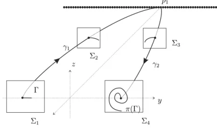
we can assume that2is contained in a neighborhood of the point p1at infinity. Let3be a small square centered at the point(−k,r2,0)and contained in the planex = −k. Hence, again we can suppose that3 is contained in a neighborhood of p1. Finally, let4be a small square centered at the point(0,r2,0)and contained in the planex =0.
Σ1 Σ4
Σ2
Σ3
γ1
γ2
Γ
π(Γ) z
y p1
Fig. 4 – The Poincaré map.
We denote byπthe Poincaré map going from1to4. Such a Poincaré map exists due to the existence of the heteroclinic loopLand to the local phase portrait on the center manifold of p1, see Proposition 3. We splitπinto three pieces. Letπ1: 1→2,π2: 2→3andπ3: 3→4. Therefore,π=π3◦π2◦π1. See Figure 4.
Letδ >0 but small. We consider the open segmentŴ =
(0,y,0): r1 < y < δ+r1
on they-axis having the left endpoint at(0,r1,0). Then, sinceπ1is a diffeomorphism (because the orbits going from1 to2use only a bounded time),π1(Ŵ)is an arc in2having the left endpoint at(−k,r1,0).
We assume that 2 and3 are in a neighborhood of p1 where the local phase portrait studied in Subsection 2.2 holds. That is,γ1andγ2are in the center manifold of p1drawn in Figure 1, and the flow outside this center manifold tends exponentially to it. Therefore, by Proposition 3,(π2◦π1)(Ŵ)is an arc in3having the left endpoint at(−k,r2,0).
Denote the time that the orbit γ2 needs to go from the point(−k,r2,0) to the point(0,r2,0)by τ. Then, ifε > 0 is sufficiently small, by the theorem on continuous dependence on initial conditions and parameters, during a finite time the flow of system (1) is close to the flow of system (1) withε = 0, and
in particularτ is close to k. So, during the timeτ ≈ k the orbits of system (1) nearγ2 passing through points of3have made approximatelyβk/2πturns (see expression (12) in Subsection 2.3). Consequently, (π3◦π2◦π1)(Ŵ)is an arc in4which spirals to the point(0,r2,0)giving approximatelyβk/2π turns. Note that the number of turns tends to infinity whenk → ∞, and we can takek as large as we want by taking the neighborhood of infinity where we choose2and3sufficiently small.
The orbits through the intersection points ofπ(Ŵ)with they-axis are periodic because, by construction, they have two points on they-axis. This completes the proof of Theorem 1.
symmetric periodic orbits. But in this note we are only interested in describing the geometrical mechanism which creates these large amplitude periodic orbits near the invariant straight linesγ1andγ2.
APPENDIX 1: POINCARÉ COMPACTIFICATION INR3
InR3we consider the polynomial differential system
˙
x = P1(x,y,z),
˙
y = P2(x,y,z),
˙
z = P3(x,y,z),
or equivalently its associated polynomial vector field X =(P1,P2,P3). The degreen ofX is defined as n=max{deg(Pi):i =1,2,3}.
LetS3= {y =(y1,y2,y3,y4)∈R4: y =1}be the unit sphere inR4, and
S+ = {y ∈S3: y4>0} and S−= {y ∈S3: y4<0}
be the northern and southern hemispheres, respectively. The tangent space toS3at the point yis denoted byTyS3. Then, the tangent plane
T(0,0,0,1)S3= {(x1,x2,x3,1)∈R4: (x1,x2,x3)∈R3}
is identified withR3.
We consider the central projections
f+: R3 = T(0,0,0,1)S3S+ and f−: R3 = T(0,0,0,1)S3S−,
defined by
f+(x) =
1
x(x1,x2,x3,1) and f−(x) = − 1
x(x1,x2,x3,1) , where
x =
1+
3
i=1 xi2
1/2
.
Through these central projections,R3 can also be identified with the northern and southern hemispheres. The equator ofS3isS2= {y∈S3: y4=0}. Clearly,S2can be identified with the infinity ofR3.
The maps f+and f−define two copies of X, one D f+◦X in the northern hemisphere and the other
D f−◦X in the southern one. Denote by X the vector field onS3\S2 =S+∪S−which restricted toS+
coincides withD f+◦X and restricted toS−coincides withD f−◦X.
introduced this compactification for polynomial vector fields inR2, and its extension toRm can be found in (Cima and Llibre 1990).
The expression for X(y)onS+∪S−is
X(y) = y4
1−y12 −y2y1 −y3y1
−y1y2 1−y22 −y3y2
−y1y3 −y2y3 1−y32
−y1y4 −y2y4 −y3y4
P1 P2 P3 ,
where Pi = Pi(y1/|y4|,y2/|y4|,y3/|y4|). Written in this way X(y)is a vector field inR4tangent to the sphereS3.
Now we can extend analytically the vector field X(y)to the whole sphereS3by
p(X)(y) = y4n−1X(y);
this extended vector field p(X)is called the Poincaré compactification ofX.
AsS3is a differentiable manifold, to compute the expression for p(X)we can consider the eight local charts(Ui,Fi), (Vi,Gi)whereUi = {y ∈ S3: yi > 0}, andVi = {y ∈ S3: yi < 0}fori = 1,2,3,4; the diffeomorphisms Fi: Ui → R3 and Gi: Vi → R3 fori = 1,2,3,4 are the inverses of the central projections from the origin to the tangent planes at the points(±1,0,0,0),(0,±1,0,0),(0,0,±1,0)and (0,0,0,±1), respectively. We now do the computations onU1. Suppose that the origin (0,0,0,0), the point(y1,y2,y3,y4)∈S3and the point(1,z1,z2,z3)in the tangent plane toS3at(1,0,0,0)are collinear, then we have
1 y1 = z1 y2 = z2 y3 = z3 y4, and consequently
F1(y) = y2 y1, y3 y1, y4 y1
= (z1, z2, z3)
defines the coordinates onU1. As
D F1(y) =
−y2/y12 1/y1 0 0
−y3/y12 0 1/y1 0
−y4/y12 0 0 1/y1
and y4n−1 =
z3 z
n−1
,
the analytical fieldp(X)becomes
zn 3 (z)n−1
−z1P1+P2,−z2P1+P3,−z3P1,
wherePi = Pi(1/z3,z1/z3,z2/z3).
In a similar way we can deduce the expressions of p(X)inU2andU3. These are
zn3 (z)n−1
−z1P2+P1,−z2P2+P3,−z3P2
wherePi =Pi(z1/z3,1/z3,z2/z3)inU2, and z3n
(z)n−1
−z1P3+P1,−z2P3+P2,−z3P3
,
wherePi =Pi(z1/z3,z2/z3,1/z3)inU3.
The expression for p(X)inU4isz3n+1P1,P2,P3where Pi = Pi(z1,z2,z3). The expression for p(X)in the local chartVi is the same as inUi multiplied by(−1)n−1.
When we shall work with the expression of the compactified vector field p(X)in the local charts we shall omit the factor 1/(z)n−1. We can do that through a rescaling of the time.
We remark that all the points on the sphere at infinity in the coordinates of any local chart havez3=0.
ACKNOWLEDGMENTS
The first author is partially supported by a MCYT/FEDER grant number MTM2005-06098-C02-01 and by a CICYT grant number 2005SGR 00550. Both authors are partially supported by the joint project CAPES-MECD grant HBP2003-0017.
The authors thank the referees for their suggestions which allowed them to improve the presentation of this paper.
RESUMO
Neste trabalho estudamos uma classe de campos vetoriais polinomiais com simetria, definidos no R3e dependendo
de um parâmetro realε, que possui um conjunto de retas invariantes paralelas que tendem para dois pontos singulares
no infinito, formando ciclos heteroclínicos degenerados. A análise global na vizinhança dos pontos no infinito é desenvolvida utilizando-se a compactificação de Poincaré. Provamos que para todon ∈Nexisteεn>0 tal que, para todo 0< ε < εn, o sistema considerado possui pelo menosnórbitas periódicas de grande amplitude, que bifurcam do ciclo heteroclínico formado pelas duas retas invariantes mais próximas do eixo-x, uma contida no semi-espaço
y>0 e a outra contida no semi-espaçoy<0.
Palavras-chave:ciclo heteroclínico infinito, órbitas periódicas, sistemas reversíveis.
REFERENCES
ANDRONOV AA, LEONTOVICHEA, GORDON II AND MAIERAL. 1973. Qualitative Theory of Second-Order Dynamical Systems. J Wiley & Sons, New York.
ARNOLD VI. 1980. Geometrical Methods in the Theory of Ordinary Differential Equations. Graduate Texts in Mathematics. Springer-Verlag, New York, 60.
CARRJ. 1981. Applications of centre manifold theory. Applied Math Sciencies, Springer-Verlag, New York, 35.
CHOWSNANDHALEJK. 1982. Methods of bifurcation theory. Grundlehren der Mathematischen Wissenschaften (Fundamental Principles of Mathematical Science). Springer-Verlag, New York, 251.
CIMAAANDLLIBREJ. 1990. Bounded polynomial vector fields. Trans Amer Math Soc 318: 557–579.
GUYONE, HULINJPANDPETITL. 1991. Hydrodynamique physique. InterEditions/Editions du CNRS.
LLIBREJ, MACKAYRSANDRODRÍGUEZG. 2004. Periodic Orbits Passing Near Infinity (preprint).
NEWELLAC, RANDDAANDRUSSELLD. 1988. Turbulent transport and the random ocurrence of coherent events. Phys D 33: 281–303.
SPARROWCANDSWINNERTON-DYERHPF. 1995. The Falkner-Skan equation I. The creation of strange invariant sets. J Differential Equations 119: 336–394.