A Framework for Efficient Model Transformations

(1)

Cláudio Ângelo Gonçalves Gomes

Bachelor

A Framework for Efficient Model

Transformations

Dissertação para obtenção do Grau de Mestre em Engenharia Informática

Orientador :

Vasco Amaral, Prof. Auxiliar,

Universidade Nova de Lisboa

Co-orientador :

Bruno Barroca, Doutorado,

Universidade Nova de Lisboa

Júri:

Presidente: Prof. Doutor Pedro Medeiros

Arguente: Prof. Doutor Juan de Lara

(2)

(3)

iii

A Framework for Efficient Model Transformations

Copyright c Cláudio Ângelo Gonçalves Gomes, Faculdade de Ciências e Tecnologia,

Universidade Nova de Lisboa

(4)

(5)

(6)

(7)

Acknowledgements

I want to thank my supervisor Vasco Amaral for sharing his experience and knowledge throughout this thesis and long before that, in lectures, conferences, etc. . .

I owe many of the ideas presented in this thesis to the discussions I had with Bruno Barroca and for that, thank you Bruno.

(8)

(9)

Abstract

The reported productivity gains while using models and model transformations to develop entire systems, after almost a decade of experience applying model-driven ap-proaches for system development, are already undeniable benefits of this approach. How-ever, the slowness of higher-level, rule based model transformation languages hinders the applicability of this approach to industrial scales. Lower-level, and efficient, lan-guages can be used but productivity and easy maintenance seize to exist.

The abstraction penalty problem is not new, it also exists for high-level, object ori-ented languages but everyone is using them now. Why is not everyone using rule based model transformation languages then?

In this thesis, we propose a framework, comprised of a language and its respective environment, designed to tackle the most performance critical operation of high-level model transformation languages: the pattern matching. This framework shows that it is possible to mitigate the performance penalty while still using high-level model transfor-mation languages.

Keywords: Model Transformations, DSL, Language Design, Pattern Matching, Model

(10)

(11)

Resumo

Os aumentos de produtividade reportados ao longo quase uma década de utilização de modelos e transformações entre modelos para desenvolver sistemas complexos cons-tituem uma prova irrefutável dos benefícios desta abordagem. Conduto, a lentidão na execução de transformações expressas em linguagens de alto nível, baseadas em regras, prejudica muito a applicabilidade da abordagem. As linguagens de baixo nível, que são muito rápidas, podem ser usadas mas nesse caso não se consegue produtividade e fácil manutensão das transformações.

Este problema da abstração não é novo. Também as linguagens orientadas por objec-tos passaram pelo mesmo mas hoje em dia toda a gente as usa. Então porque é que não acontece o mesmo com as linguagens de transformação? O que falta fazer?

Nesta tese, propomos uma linguagem de transformação e respectivo ambiente de suporte, concebida para contornar o maior obstáculo à aplicabilidade industrial das lin-guagens de transformação de alto nível: a captura de padrões. Com a nossa abordagem demonstramos que é possível mitigar o problema da abstração.

Palavras-chave: Transformações de Modelos, Linguagens de Domínio Específico,

(12)

(13)

List of Figures

2.1 Questionnaire model. Taken from [ABDT10]. . . 6

2.2 Questionnaire metamodel. Taken from [ABDT10]. . . 8

2.3 Questionnaire model and metamodel. Taken from [ABDT10]. . . 9

2.4 (Highly) Simplified Ecore Metamodel. . . 10

2.5 (Partial) Relations of conformance between model, metamodel and meta-metamodel. . . 11

2.6 System, Model, metamodel and meta-metamodel. . . 12

2.7 Simplified EJB model generated from a questionnaire model. . . 12

3.1 Example rule used to specify a model transformation. . . 13

3.2 Overview of the model transformation process.. . . 14

3.3 Excerpt of a transformation expressed in DSLTrans. . . 18

3.4 Overview of the execution process of a transformation model. . . 19

3.5 Transformation running times of some state of art tools. . . 19

4.1 Sample input model (left) and corresponding metamodel (right). . . 22

4.2 Sample pattern. . . 22

4.3 Example occurrence of the Left-Hand-Side (LHS) pattern of the rule in Fig-ure 3.1. . . 23

5.1 Programming languages benchmark on sudoku solving. Taken from [Att]. 34 5.2 C Compilation Overview. . . 35

5.3 High level model transformation language compilation overview. . . 36

6.1 Proposed approach to solve the abstraction penalty. . . 38

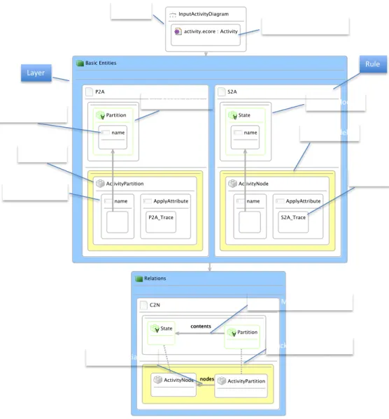
6.2 Excerpt of TrNet metamodel - top level elements (simplified). . . 39

6.3 TrNet sample transformation labelled. . . 39

6.4 Excerpt of TrNet metamodel - nodes and edges (simplified). . . 40

(16)

xvi LIST OF FIGURES

6.6 Excerpt of TrNet metamodel - Restrictions (simplified). . . 42

6.7 Sample model with two Partition instances. . . 42

6.8 Transformation configuration after the completion of Op1. . . 43

6.9 TrNet sample transformation (continuation). . . 44

6.10 TrNet sample transformation (final configuration). . . 45

6.11 Excerpt of TrNet metamodel - Conditions (simplified).. . . 46

6.12 Excerpt of TrNet metamodel - Actions (simplified).. . . 47

6.13 Excerpt of TrNet metamodel - Calculations (simplified). . . 47

6.14 TrNet sample transformation with external action and condition calls. . . 48

6.15 TrNet sample transformation with a cycle. . . 49

6.16 Sample input model (left) and corresponding metamodel (right). . . 50

6.17 Transformation excerpt - inputs. . . 51

6.18 Transformation excerpt - outputs. . . 57

6.19 Output model build with Algorithm 12 . . . 58

6.20 DSLTrans sample transformation equivalent to the one in figure 6.10. . . . 58

6.21 Sample activity diagram model (UML 1.4). . . 59

6.22 Sample activity diagram model (UML 2.1). . . 59

7.1 TrNet transformation execution process. . . 62

7.2 TrNet common runtime. . . 62

7.3 Decomposition process classes. . . 63

7.4 Shapes metamodel (equivalent to the one in Figure 6.16b. . . 64

7.5 Transformation with input and output frontiers. . . 69

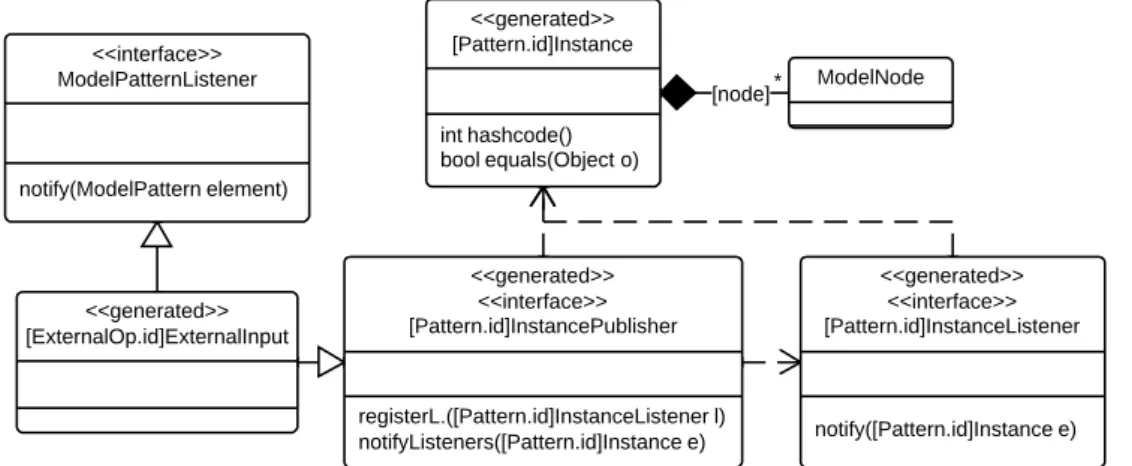
7.6 Class diagram for each class generated from a TrNet pattern. . . 70

7.7 Class diagram for each class generated from a TrNet pattern that is in the input or output frontiers. . . 71

7.8 Class diagram for classes generated from the input external operators and patterns in the input frontier. . . 71

7.9 Class diagram for classes generated from the output external operators and patterns in the output frontier. . . 73

7.10 Class diagram for the class that implement the behaviour of the transfor-mation along with the classes it relates to. . . 74

7.11 Composition process classes. . . 79

7.12 A typical TrNet transformation process. . . 87

7.13 A DSLTrans transformation and its corresponding TrNet transformation. . 89

7.14 A DSLTrans transformation and its corresponding TrNet transformation (continuation). . . 91

8.1 Transformation excerpt. . . 94

8.2 Catalog metamodel.. . . 97

(17)

LIST OF FIGURES xvii

8.4 Shapes model sample. . . 98

8.5 Catalog model sample generated from the metamodel of Figure 8.3 and the sample model of Figure 8.4. . . 98

8.6 Transformation input frontier example with statistics filled from the cata-log model of Figure 8.5.. . . 100

8.8 Example search graph and a possible search plan (in bold) for pattern of Figure 8.7 in page 103. . . 104

8.9 Weighted search graph a possible search plan (in bold) for pattern of Fig-ure 8.7 in page 103. . . 105

8.10 Expected and real number of instances of a transformation that translated Class models into Relational model, expressed in TrNet.. . . 105

8.11 Expected and real number of instances of a transformation that migrates Activity Diagram models into UML 2.0 Activity Diagrams, expressed in TrNet. . . 106

8.12 Expected and real number of instances of a transformation that migrates Activity Diagram models into UML 2.0 Activity Diagrams, expressed in DSLTrans and then compiled to TrNet. . . 106

9.1 Sample cycle with dependencies between the combinators. . . 110

9.2 Sample transformation with dependencies between the combinators and one selected execution order. . . 111

9.3 Transformation excerpt. . . 112

9.4 Example of a combinator where early evaluation of the condition is possible.114

9.5 Representation of a transformation excerpt where two patterns are redun-dant (in red). . . 116

9.6 Resulting transformation after applying the overlapped pattern matching technique to the transformation depicted in Figure 9.5. . . 117

9.7 Representation of a transformation excerpt where two operators marked in red are redundant. . . 118

9.8 Resulting transformation after applying the overlapped pattern matching technique to the transformation depicted in Figure 9.7. . . 119

9.9 Evolution of the number of patterns and number of operators in a TrNet transformation during the application of the Overlapped Pattern Matching technique. . . 120

9.10 DSLTrans Transformation sample. . . 121

9.11 TrNet Transformation sample compiled from the one in Figure 9.10. . . 121

9.12 TrNet Transformation sample after the application of Overlapped Pattern Matching. . . 122

(18)

xviii LIST OF FIGURES

10.2 UML 2.2 Activity Diagrams (based on [RKPP10b]).. . . 125

10.3 Activity migration transformation rule. . . 126

10.8 Benchmark results. . . 130

10.9 Estimated NOI for the activity migration transformation created by-hand. 130 10.10Estimated NOI for the activity migration transformation created by-hand. 131 11.1 Example of a sequential join that creates a more complex pattern. . . 134

(19)

List of Tables

(20)

(21)

Listings

7.1 Input visitor code generated from the metamodel shown in Figure 7.4 . . 63

7.2 Class generated from the patternP at4in Figure 7.5 . . . 68

7.3 Input external operator code generated from the transformation in Figure 7.5 71

7.4 Output external operator code generated from the transformation in Fig-ure 7.5 . . . 72

7.5 Transformation code generated from the transformation in Figure 7.5 . . . 75

7.6 Output visitor code generated from the metamodel shown in Figure 7.4 . 79

7.7 Typical code to run a TrNet transformation . . . 87

(22)

(23)

1

Introduction

The immersion of computer technology in a wide range of domains leads to a situation where the users’ needs become demanding and increasingly complex. Consequently, the development of successful software systems also becomes increasingly complex.

Models are an important mechanism to deal with system complexity [Sch06;KBJV06]. In the context of software engineering, models can be used to describe and prescribe en-tire systems. Therefore, a promisingdivide-and-conqueridea to break down this increasing

complexity in software engineering, is to intensively use models during all stages of soft-ware development, as in the Model Driven Development (MDD) approach.

MDD is a software engineering approach that uses models and model transforma-tions as first class citizens to create and evolve software systems [HT06]. Typically, several different models of the same system are combined across multiple levels of abstraction resulting in the implementation of that system. In MDD, both the design and develop-ment of new software systems is done by having multiple levels of abstraction, where each level deals only with a particular aspect of the system (therefore decreasing its com-plexity), and assuring the consistency between them (e.g., translations, synchronisations, etc.). In practice, each level of abstraction can be formalised by means of a domain spe-cific modelling language (DSML), and materialised by its respective supporting tools (i.e., editors, simulators, interpreters, analysers and compilers).

(24)

1. INTRODUCTION 1.1. Problem Statement

1.1 Problem Statement

In order to effectively enable MDD, the consistency between models has to be ensured by model transformations. These transformations have to be easy to specify, maintain and quick to execute. However, as we will see in the following chapters, designing a model transformation language that satisfies those three requirements is really difficult.

There are model transformation languages that are quick to execute, for instance, any general purpose programming language equipped with a proper library such as Java+EMF [Gro09]; and languages that promote productivity and maintainability, such as AGG [Tae04], Atom3 [LVA04] or Viatra2 [VB07].

The former languages are typically imperative in the sense that the user of the lan-guage specifies how the transformation is supposed to execute. The latter ones are declar-ative, where the user specifies a set of rules that relate the input models to the output models. The model transformation engine handles the other details. The rules are com-prised of a left hand side graph-like pattern and right hand side graph-like pattern. Dur-ing the transformation execution, the engine must search the input model for occurrences of the left hand side pattern and, when a match is found, an instance of the right hand side pattern is produced in the output model. Due to the graph-like representation of mod-els, searching for occurrences of some graph-like pattern is known to be an NP-Complete problem [Zün96].

This shows that there is a price to pay for increased abstraction in model transforma-tion languages. Taking that in consideratransforma-tion, our research questransforma-tion can be stated as:

How can we avoid the abstraction penalty in model transformation languages?

1.2 Expected Contributions

In this thesis we explore how to mitigate the abstraction penalty in model transformation languages. We propose a framework, comprised of a language and its respective envi-ronment, designed to tackle the most performance critical operation of high-level model transformation languages: the pattern matching.

The language proposed, instead of following a rule based approach, like most of the state of the art, represents the transformation as a network with explicit structures to control the flow of information from the input model to the output model. This explicit representation of the transformation allows for the application of several analysis and optimizations.

(25)

1. INTRODUCTION 1.3. Document Structure

1.3 Document Structure

This thesis’ structure reflects the main development steps of our solution. Each chapter is a step in achieving that solution.

The first four chapters represent our state of the art investigation. Then, Chapter5

(26)

(27)

2

Model Driven Development

This chapter is intended to make the thesis as self-contained as possible. We present all the necessary concepts to understand the context of this thesis. We start by conveying the definition of the word model and introducing the example that will be used throughout the chapter. We explain how models can be used to describe complex systems and the role of model transformations in that process. We conclude with an overview of the most used pattern matching and optimization techniques.

2.1 Models

It is by no means reasonable to build a map the same size as the city it represents. Ab-straction, along with problem decomposition and separation of concerns is one of the best ways to deal with complexity [Sch06;KBJV06]. A map of a city is an abstraction of that area that addresses a particular concern. There are several types of maps: road maps (the most widely used), economical maps, political maps, etc. . . A map is a model.

Given a systemM0, a model M1 is (i) a representation based on the system M0 (ii)

reflecting only the relevant parts ofM0(iii) to serve a given purpose [Kuh06].

In the context of software engineering, models are often represented as graphs1

be-cause graphs can express complex structures and relations; they are intuitive, expressive and suited for automatic manipulation [Ehr06]. We will be using the terms graphs and models interchangeably. UML Class Diagrams are widely used to create models of the static information in a software system.

(28)

2. MODELDRIVENDEVELOPMENT 2.2. Syntax and Semantics

Using models like the one shown in Figure2.1, social scientists, without any program-ming expertise, are able to deploy full featured web applications to conduct their studies. In order to accomplish this, these scientists use applications such aseSurveysPro2or Lime-Service3to read and translate questionnaire models into web applications [ABDT10].

Figure 2.1: Questionnaire model. Taken from [ABDT10].

In technical terms, one of the ways to serialize a model is through the XML Metadata Interchange (XMI) format [Om02]. XMI is a standard XML format created to enable both human and machine readable representation of models.

How does one guarantee that social scientists will always build syntactically correct questionnaire models? By syntactically correct we mean that they are suited for being parsed by some application. Note that a successfully parsed questionnaire does not have to make any sense. We will discuss syntax and semantics in the next section.

2.2 Syntax and Semantics

In order to better understand syntax and semantics consider the following example:

The expression “5

0” is syntactically correct with respect to integer

arith-metic because “5” and “0“ are valid integers and the division is a binary

op-erator; but semantically incorrect since “5

0” does not mean anything or has

(29)

2. MODELDRIVENDEVELOPMENT 2.3. Metamodels

the wrong meaning. The expression “5∗3” is syntactically and semantically correct: it means “15”. The expression “5+” is syntactically incorrect because

the plus operator needs two operands.

A syntactically correct model has to respect some well-formedness rules. A semanti-cally correct model can be interpreted to produce something with meaning.

Since models are to be automatically parsed and interpreted, there must be a way to unambiguously specify well-formedness rules. That is were a metamodel comes in.

2.3 Metamodels

A metamodel is a set of rules that describes all possible syntactically correct models, i. e., given a modelM1 and a metamodelM2 ofM1, it is easy to check ifM1 is syntactically

correct with respect to M2 [KBJV06]. When this happens, we say that M1 conforms to M2. Moreover, givenM2, a computer is able to parse anyM1, that conforms toM2, and

further do something useful with that information. This is analogue to what happens between a program and its programming language. The program has to be parsed by some compiler (or interpreter), hence the need for a set of rules dictating syntactically correct programs.

Figure2.2shows a simplified metamodel for questionnaire models. This metamodel can be used by applications that parse questionnaire models to check if they are syntac-tically correct. As the questionnaire metamodel shows, a questionnaire is formed by a forest of blocks. Each block contains a set of questions with zero or more options. Ques-tions with zero opQues-tions expect any textual answer. A questionnaire has attributes such as title, introduction, logo, appreciation text, acknowledgements and an expected time to complete. The information about the each particular metamodel element lies in its attributes. Comparing the model shown in Figure2.1and the metamodel of Figure2.2

one is able to determine to determine the correspondence between each model element and metamodel element. For instance, theSchoolViolenceelement corresponds to aBlock. This relation between a model element and its corresponding metamodel elements is the

instance of relation. In our example, theSchoolViolenceis an instance of theBlockelement.

Formally, a modelM1conforms to a metamodelM2iif it is possible to build ainstanceof

relation between the set of nodes and associationsN1andA1of modelM1and the set of

nodes and associationsN2andA2ofM2such that the following conditions hold:

∀a∈A1instanceof(src(a)) =src(instanceof(a))

∀a∈A₁instanceof(trg(a)) =trg(instanceof(a))

wheresrc(a)andtrg(a)denote the source and target elements of the associationa. For

(30)

2. MODELDRIVENDEVELOPMENT 2.4. Meta-metamodels

Figure 2.2: Questionnaire metamodel. Taken from [ABDT10].

Figure2.3shows theinstanceofrelation between the model of Figure2.1and the

meta-model of Figure2.2.

There are tools called modelling environments that offer support to the creation of metamodels and tools to manipulate models. For instance, a user can use a modelling environment to create a questionnaire metamodel like the one shown in figure 2.2and automatically generate a set of editors that ease the manipulation of questionnaire mod-els. Eclipse Modeling Framework (EMF) [Gro09] is an example of a modelling environ-ment but there are others such as Generic Modelling Environenviron-ment (GME) [LBMVNSK01] or MetaEdit+ [TR03].

How does the modelling environment guarantees that the created metamodels are syntactically correct? Where are the set of rules that prescribe well formed metamodels?

2.4 Meta-metamodels

A metamodelM2conforms to a meta-metamodelM3. A meta-metamodel represents the

set of all well formed metamodels. Note that this makes the metamodel a model M2

conforming to M3. Figure2.4 shows a simplification of a meta-metamodel: the Ecore

meta-metamodel. The Ecore is the meta-metamodel used in the Eclipse Modelling Envi-ronment (EMF).

The relation between a metamodelM2 and a meta-metamodelM3is the same as the

one between a model M1 and M2: M2 is an instanceof M3. The instanceof relation is

(partially) shown in Figure2.5.

(31)

2. MODELDRIVENDEVELOPMENT 2.5. Model Driven Development

Figure 2.3: Questionnaire model and metamodel. Taken from [ABDT10].

the level of metamodels and below [Fav04]. Figure2.6summarizes the four levels of ab-straction described until now. TheM0 denotes the system under study that needs and

abstraction;M1denotes the model ofM0;M2is the metamodel to whichM1conforms to;

andM3 is the meta-metamodel.

2.5 Model Driven Development

Model-Driven Development (MDD) is a software engineering approach that uses mod-els as first class citizens to create and evolve software systems [HT06]. The software code is generated from a set of models thus enabling massive reuse and “correct-by-construction” software [Sch06].

The Model-Driven Architecture (MDA) is a set of guidelines proposed by the Object Management Group4_{(OMG) on how to produce applications using MDD [}_Sol00_{]. These}

guidelines suggest that when building a complex system, Platform Independent Models (PIMs) should be used to describe that system. Then, PIMs are translated to Platform Specific Models (PSMs). Furthermore, MDA proposes a meta-metamodel (M3) called

Meta Object Facility (MOF) and the four abstraction levels shown in Figure2.6.

Platform Independent Models (PIMs) denote those models that don’t keep specific

(32)

Figure 2.4: (Highly) Simplified Ecore Metamodel.

information about a system’s ultimate execution environment (operating system, pro-gramming language, etc. . . ) [AK05]. The questionnaire model of Figure 2.1 does not keep information about its execution environment, i.e., it is a PIM. Because of this, an application like eSurveyPro can choose to generate a web application or a desktop appli-cation, or even a mobile version, to evaluate the survey.

After a total or partial specification of the necessary PIMs to describe a system, a set of Platform Specific Models (PSMs) is generated from those PIMs. PSMs carry information about the system’s execution environment and are well suited for being used to generate (automatically or semi-automatically) that system.

An application like eSurveyPro, capable of processing a questionnaire model to pro-duce a web application, would operate in the following way:

1. A questionnaire model is given as input to the application;

2. The application checks if the model conforms to the questionnaire metamodel. 3. Assuming the model is syntactically correct, there are three equivalent alternatives:

(a) The application interprets the model and presents the user with a web page containing the questions and choices declared in the model.

(b) The application translates the model to a set of Java classes that, when run, present the user with a web page containing the questions and choices de-clared in the model.

(c) the application translates the questionnaire model to a Enterprise JavaBeans (EJB) model5 _{and then the EJB model is translated to a set of classes}

imple-menting the questionnaire. The classes generated include support for trans-actions, remote and distributed execution, persistence, etc. . . This EJB-to-Java translation is done by other application (e.g.,AndroMDA6is a tool capable of

(33)

Figure 2.5: (Partial) Relations of conformance between model, metamodel and meta-metamodel.

performing the translation), specifically devised to translate EJB models to ex-ecutable Java classes.

The alternatives 3a, 3b and 3c have the same purpose: they provide semantics (a meaning) to the questionnaire model. The first alternative gives semantics in an opera-tional manner. The second and third ones do this through a transformation into a model that already has defined semantics (EJB is a model and code can also be seen as a model [Béz05]).

The alternative3cis theeasiestto realize because the transformation we have to build

is one between models conforming to similar metamodels (Questionnaire and EJB) as to building an interpreter or a compiler (options3a and3b). Option 3cis also thesafest

alternative because the probability of introducing bug in the transformation process is far smaller than in the other options. Figure2.7shows a possible (simplified) EJB model produced with such a transformation applied to the questionnaire model of Figure2.1. By observing the EJB model, we can immediately come up with a set of heuristics on how to perform the transformation: 1. Each questionnaire item is translated into aSession Beanand a persistedEntity Bean. TheSession Beanobjects provide the necessary controls to allow the user to answer the questionnaire. 2. Blocks, Questions and Options are all translated into respectiveEntitiesas they need to be persisted after each session.

The keen reader will observe that the heuristics presented are applicable to any pos-sible questionnaire model, not just the one shown in Figure2.1.

(34)

Figure 2.6: System, Model, metamodel and meta-metamodel.

Figure 2.7: Simplified EJB model generated from a questionnaire model.

(35)

3

Model Transformations

A model transformation is “the automatic generation of a target model from a source model, according to a transformation definition” [KWB03].

The transformation definition is expressed in some language. The language can be a general purpose language like Java or a more specific model transformation language.

Model transformation languages, together with their supporting model tion tools provide an high-level and highly productive environment where transforma-tion specificatransforma-tions consist of rules like the one shown in Figure3.1.

Figure 3.1: Example rule used to specify a model transformation.

3.1 Environment

(36)

3. MODELTRANSFORMATIONS 3.2. DSLTrans - A Model Transformation Language

metamodel. Typically, even the transformation itself is a model conforming to a meta-model [Béz04] as is illustrated in Figure3.2.

Figure 3.2: Overview of the model transformation process.

The MMM denotes the meta-metamodel (e.g. Ecore or MOF) and the MMt is the

metamodel of the transformation specification. This metamodel, MMt, is often called

the transformation language. Note that if n = m = 0 and MM0 = MM′0 we have a

transformation between models conforming to the same metamodel, i. e., an endogenous transformation [MVG06]. When the input and output metamodels are different we have an exogenous transformation [MVG06].

There is a great variety of MTTs, each unique in features provided, language used, and approach followed to solve the model transformation problem [GGZVEVGV05]. Some operate with just a set of transformation rules applying them in any order (declarative approaches); others allow the user to control rule scheduling (or rule selection) (hybrid approaches); others take this further by providing an imperative language with loop constructs, branching instructions, composition mechanisms, etc. . . that allow the user to program all the transformation process (imperative approaches). Czarnecki and Helsen provided a classification of model transformation approaches in [CH03] that captures most of the MTTs’ features from a usability point of view.

3.2 DSLTrans - A Model Transformation Language

(37)

3. MODELTRANSFORMATIONS 3.3. State of Art

A transformation in DSLTrans is formed by a set of input model sources called file-ports (“inputQuestionnaire” in Figure3.3) and a list of layers. Input model sources are typed by the input metamodel and layers are typed by the output metamodel. Each layer is a set of rules that are executed in a non deterministic fashion. The top part of each rule is called the “match” and the bottom is “apply”.

In the example presented in Figure 3.3, in the first layer, left rule, for each Question instance found in the input model, a new EntityBean instance is created in the output model, with the name “Question” and id equal to the id of the found Question instance. In addition, a trace link is created internally identified by the “Q2E_Trace” string. These trace links can be used in the subsequent layers to retrieve a Question instance and the corresponding EntityBean instance created in the rule. In the right rule, a similar opera-tion is performed to all the Opopera-tion instances found in the input metamodel. In the rule of the second layer, all the question and respective offered questions are being matched in the input model, together with the corresponding previously created EntityBeans and a new association called “first" is being created.

For more details about DSLTrans, please refer to section6.2in chapter6.

3.3 State of Art

Off course DSLTrans is not the only model transformation language. There are many others, each with it’s particular set of features, advantages and limitations. In our study, we tried to cover as much languages as possible, namely: (i) imperative tools such as ATC [EPSR06] and T-Core [SV10]; (ii) declarative tools such as AGG [Tae04], Atom3 [LVA04] and Epsilon Flock [RKPP10a]; (iii) programmed graph rewriting approaches such as GReAT [BNBK07], GrGen.NET [KG07], PROGReS [Sch94], VMTS [LLMC05] and MoTif [SV11]; (iv) incremental approaches such as Beanbag [XHZSTM09], Viatra2 [VB07] and Tefkat [LS06]; (v) and bidirectional approaches such as BOTL [BM03a].

3.4 The Model Transformation Process

Based on our study of the state of the art tools, we built a general process that identifies the main stages occurring in most model transformation executions.

Figure3.4identifies the main stages in two typical transformation execution modes: interpretation (left) and compilation (right). The only difference between these two modes is that, in the compilation, the execution of the transformation is separated from the trans-formation load, parse and compile tasks and off course, the performance, as we will see in chapter10.

(38)

3. MODELTRANSFORMATIONS 3.5. Performance

the transformation execution stages (in the Execute Transformation State) are manually coded by the transformation programmer. We also assume that a transformation is com-prised of a set of rules, each containing an Left-Hand Side (LHS) pattern, that needs to

be found in the input model, and a Right-Hand Side (RHS) pattern which represents the output model. There is no loss of generality, since theserules(with the mentioned

pat-terns) do not need to be explicitly represented in the transformation language. They can be implicit in the transformation programmer’s mind when coding the transformation. For simplicity’s sake, we only consider one input model and one output model but it is easy to see how the process can be adapted to multiple input/output models.

As is illustrated in Figure3.4, an engine always starts by loading the transformation and, in the case of interpretation, the input model. At this point, some existing engines perform global optimizations, which will be explained and categorized in section 4.2. Next, the engine executes the transformation by selecting each rule and optionally per-forming some local optimizations (see section4.2). After those optimizations, a search in the input model must be performed in order to find where to apply the rule. In this task, the engine has to find occurrences of the rule’s left-hand side pattern in the input model. From a performance point of view, this operation is the most expensive, and usually all the optimizations target the reduction of its cost (see chapter4). The application of the rule’s right hand side is performed for each occurrence found and, if there are more rules to be applied, the transformation continues. Else, the transformation execution ends. After that, the output model is stored.

3.5 Performance

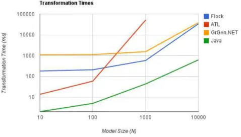
In order to better understand how much the pattern matching operation (theMatch LHS

State in Figure 3.4) costs, we picked a benchmark created for the Tool Transformation Contest (TTC) 2010. For all details about the benchmark case study, input models and tools used, please refer to chapter10.

From the available submissions we selected transformations expressed in Epsilon Flock, ATL and GrGen.NET tools. We also coded a transformation entirely in Java, using the Eclipse Modelling Framework (EMF) library to load and store the models.

Running each transformation with increasingly larger input models yielded the re-sults shown in Figure 3.5. Note the logarithmic scale in both axes. The vertical axis denote the total transformation time, i.e., the input model load, transformation parse, execution and output model storage tasks. The horizontal axis denotes the input model size.

(39)

languages, a tiring, unproductive and error-prone task. Not to mention that the code is tightly coupled to the EMF library to load and store models.

The three tools used have a very intuitive, compact and declarative syntax to specify the transformation. Compared to Java, it is really easy and quick to create the transforma-tion in all three languages. Also it should be straightforward to cope with any change to the representation of models. The problem is that at industrial scales, any transformation written in these languages becomes useless.

Only after high-level transformations are shown to run fast enough, people will use them at industrial scales. Optimization techniques play an important role for that pur-pose.

(40)

(41)

(a) Interpretation process of a

transfor-mation model overview. (b) Compilation process of a transfor-mation model overview.

Figure 3.4: Overview of the execution process of a transformation model.

(42)

(43)

4

Pattern Matching Optimization

Techniques

In this chapter, we study the pattern matching process. Optimizing this NP-Complete [Zün96] problem is one of the most effective ways to reduce execution times and achieve industrial applicability for model transformations. We identify and classify several pat-tern matching optimization techniques and we present the categorization of the state of the art tools.

In the following sections we provide a simple and general explanation for each opti-mization technique with the help of some examples. The input model used, and corre-sponding metamodel, are presented in Figure4.1. The metamodel states that instances of

Mare comprised of zero or more instances ofA.Aelements refer to zero or more elements

of typeBor C.Celements may reference multipleCinstances. All elements have an id

string attribute andCelements have an extraccsinteger attribute. Note that containment

associations (with the black diamond in the source) state that a child element (association target) may only exist inside one parent element (association source). Later we will see why this fact has an impact on the performance of the pattern matching operation.

4.1 The Pattern Matching Problem

(44)

4. PATTERNMATCHINGOPTIMIZATIONTECHNIQUES 4.1. The Pattern Matching Problem

(a) Model used as input for the

illustra-tion of pattern matching techniques. (b) Metamodel.

Figure 4.1: Sample input model (left) and corresponding metamodel (right).

example, there are two: the first one is shown in the figure and the second one has the mapping{(x, a3),(z, c3),(y, b3)}. Had we omitted the restrictionccs=2and there would

be 6 possible mappings.

Figure 4.2: Sample pattern.

In order to find such mapping in any given input model, a transformation engine has to follow an algorithm similar to Algorithm1. A few remarks about the notation: 1. The

GetAllInstances(Type)function returns the set of all elements from the input model that are

instances ofType; 2.element.associationreturns, all the model elements that are connected

toelementby the associationassociationas targets; 3.element.attributereturns the value of

the attributeattributeof the elementelement; 4. It should be clear by the context whether

we are navigating an association or accessing an attribute with these two last operations; 5. TheBACunique identifies the pattern in Figure4.2;

The algorithm starts by finding all the instances ofAand then, for each instance a,

navigates along the edgesa.abanda.acto find the remaining elements.

For the worst case scenario, assume thatGetAllInstances(T)has to search through the

entire model to find all elements of typeTand assume thatAelements are connected to

everyBand everyCelements in the model. The time complexity of the Algorithm1, in this scenario, isO(((|M|+|A|+|B|+|C|) + (|A| × |B| × |C|))where|T|denotes the size of

(45)

4. PATTERNMATCHINGOPTIMIZATIONTECHNIQUES 4.1. The Pattern Matching Problem

Figure 4.3: Example occurrence of the Left-Hand-Side (LHS) pattern of the rule in Fig-ure3.1.

Algorithm 1An algorithm to find occurrences of the pattern shown in Figure4.2. functionFINDALLOCCURRENCESBAC

occurrences← {}

fora∈GetAllInstances(A)do forb∈a.abdo

forc∈a.acdo ifc.ccs= 2then

occurrences←occurrences∪ {(x, a),(y, b),(z, c)} end if

end for end for end for

returnoccurrences

end function

operation. In a whole transformation execution, several patterns need to be matched. Most model transformation tools, when loading the input model (see the process in figure3.4), create an index to store elements organized by their type. Using this feature the tool does not have to search the whole input model to find an element of a given type1_{. This causes the}_{GetAllInstances(T)}_{function to return immediately with the set of}

all instances ofT. So, the worst case, for most model transformation tools, of Algorithm1

isO(|A| × |B| × |C|).

In general, given an arbitrary pattern with{n1, n2, . . . , nm}matching elements, each

being instance of types {T1, T2, . . . , Tm}, respectively, an algorithm to match those

ele-ments has a worst case time complexity ofO(|T1| × |T2| ×. . .× |T_m|). Note that ifT_i=T_j

for alliandj, we haveO(Tm₎_{meaning that the algorithm is exponential in the size of}

the pattern.

(46)

4. PATTERNMATCHINGOPTIMIZATIONTECHNIQUES 4.2. Optimization Techniques

4.2 Optimization Techniques

The good news is that, in the model transformation context, models are typically sparsely connected, model elements are indexed by their type and patterns in rules are generally small. Because of these facts, the average pattern matching process has a complexity that can be “(. . . ) overapproximated by a linear or quadratic function of the model size” [VFVS08]. Also, there is lots of room for improvement in Algorithm1.

4.2.1 Indexing Techniques

For instance, the tool could be improved to, when loading the input model, create an index with the inverse associations of the existing associations. This feature is so useful that it is usually supported by the model management frameworks used by tools, such as UDM [MBLPVAK03] or EMF [Gro09]. It also means that, for each instance of an as-sociationT1

assoc

−−−→T2, there would be an instance of the associationT2

assocInv

−−−−−→T1. The

implications are clear: If there are only associationsT1 assoc

−−−→T2in the model and we are

given an elementt2 instance ofT2, it is still possible to obtain all the instances ofT1 that

are connected tot2 without having to search all instances ofT1in the model. We do that

with t2.assocInv. If an engine supports this indexing technique, then the Algorithm 1

could be improved to Algorithm2.

Algorithm 2An algorithm to find occurrences of the pattern shown in Figure4.2taking

advantage of inverse associations.

functionFINDALLOCCURRENCESBAC

occurrences← {}

forc∈GetAllInstances(C)do ifc.ccs= 2then

fora∈c.acInvdo forb∈a.abdo

occurrences←occurrences∪ {(x, a),(y, b),(z, c)} end for end for end if end for returnoccurrences end function

In Algorithm2we switched the order of the loops because, since we can only have an occurrence if thezelement satisfies the restrictionz.ccs = 2, we might as well start by

looking for such zelements. Notice that we can only take advantage of this heuristic if

the engine has built inverse relations.

(47)

that satisfies the restrictionz.ccs = 2. In Chapter8we will show how this probability can be estimated. For now, if the input model shown in figure 4.1ais representative, then

P(z.ccs= 2) = 13.

We can improve the indexing techniques of the tool to provide attribute indexes. This way, if an elementT with an attributeT.attrof typeP is frequently accessed throughout

a transformation, then building an index Tattr : P → T can yield a major speed up.

Algorithm 3 shows how this index can be used to fetch immediately all the instances

cof C satisfying the restriction c.ccs = 2. Note that since the index fetches the correct instances there is no need for the verification of the restriction. Normally, the creation of these indexes is controlled by the user so that only the most relevant attributes are indexed but the tool can analyse all the transformation and determine which attributes deserve to be indexed. In order to fill the index with the necessary instances, the tool, when loading the input model, scans allCinstances and organize them in the index.

Algorithm 3An algorithm to find occurrences of the pattern shown in Figure4.2taking

advantage of attribute indexes.

occurrences← {} forc∈Cccs(2)do

fora∈c.acInvdo forb∈a.abdo

occurrences←occurrences∪ {(x, a),(y, b),(z, c)} end for

end for end for

end function

We can take these indexing techniques one step further and implement structural indexes. These allow for the storage of instances of whole patterns. For example, assume that the patternB ←−ab A−→ac C, identified byBAC’is frequently matched throughout the

transformation. By detecting this fact, the engine creates an indexIBAC′ :B×A×Cthat,

when accessed, returns all the instances of that pattern. Algorithm4shows an example match operation that uses the structural index that we gave as example. Similarly to the previous indexing techniques, the engine has to fill the index after loading the model, and particularly for this indexing technique, this operation can be costly. But the average cost of Algorithm4lowers toO(|IBAC′| ×P(z.ccs= 2)). Normally, the creation of structural

(48)

4. PATTERNMATCHINGOPTIMIZATIONTECHNIQUES 4.2. Optimization Techniques Algorithm 4An algorithm to find occurrences of the pattern shown in Figure4.2taking

advantage of structural indexes.

occurrences← {} for(b,a,c)∈IBAC′do

ifc.ccs= 2then

occurrences←occurrences∪ {(x, a),(y, b),(z, c)} end if

end for

end function

Up until know we have seen three indexing techniques: Type, Attribute and Struc-tural. These techniques are applied automatically by the engine, all the necessary struc-tures are initialized in the “Perform Global Optimizations” stage of the transformation process of Figure3.4, and they impact more than one pattern matching operation. That is why we call them global optimizations as opposed to local ones, in which the impact is on the current pattern matching operation.

4.2.2 Caching

Yet another global optimization technique, similar to indexing, is to cache pattern match-ing operations. This can be performed automatically by detectmatch-ing which match opera-tions’ results can be reused in other operations. TheCache act as a map that returns all

instances of a given pattern identifier. For instance, consider Algorithm 5 that imple-ments the look up for the pattern of Figure4.4. Note how the cache is being accessed and updated. If all the pattern matching algorithms used in the transformation behave the same way with respect to the cache, then the matching of the pattern of Figure4.4could be matched by Algorithm6. If the engine matches the pattern of Figure4.4before match-ing the one of Figure4.2, then Algorithm6will always hit the cache and only iterates the

Cinstances. Note thatABis a unique identifier for the pattern in Figure4.4and thatBAC

is a unique identifier for the pattern in Figure4.2.

Caching techniques serve not only the purpose of storing patterns. For instance, they can be used to store derived attributes2 _{as is done in ATL [}_JABK08_{]. Derived attributes}

can be computed and stored when loading the input model.

Figure 4.4: Sample pattern.

(49)

Algorithm 5An algorithm to find occurrences of the pattern shown in Figure4.4using

cache.

functionFINDALLOCCURRENCESAB ifCache[AB]=∅then

occurrences← {}

fora∈GetAllInstances(A)do forb∈a.abdo

occurrences←occurrences∪ {(x, a),(y, b)} end for

end for

Cache[AB]←occurrences

end if

returnCache[AB]

end function

cache.

functionFINDALLOCCURRENCESBAC ifCache[BAC]=∅_then

occurrences← {}

for{(x, a),(y, b)} ∈Cache[AB]do forc∈a.acdo

end for

Cache[BAC]←occurrences

end if

returnCache[BAC]

(50)

4. PATTERNMATCHINGOPTIMIZATIONTECHNIQUES 4.2. Optimization Techniques 4.2.3 Search Plan Optimization

Algorithm2presents a different loop order to take advantage of thez.ccs=2restriction in

pattern of Figure4.2. The argument is that the average cost of the whole pattern matching operation is less than the cost of Algorithm 1. This is true but for an engine to reason about such things there must be a notion of plan and cost.

Generically, a search plan [VFVS08;Zün96] for a pattern is a representation of the al-gorithm to be performed to find occurrences for that pattern. Changes to the search plan imply changes to the algorithm. A search plan with a lower cost, implies that the algo-rithm, in the average case, should have a lower cost. Search plan optimizations are local because, each time they are applied, they attempt to reduce the cost of each individual pattern matching optimization.

Each model transformation tool that implements search plan optimizations has its own representation of a plan, and cost. But in the tools that we studied we were able to identify three kinds of cost models, which we named according to the kind of information they require. There are cost models that take into account a sample of representative in-put models, the current (under transformation) inin-put model, the inin-put metamodel struc-ture and even the cost of the underlying strucstruc-tures such as index look ups, disc access, etc.

A cost model that only requires information about the metamodel is called metamodel sensitive. It employs a set of heuristics that take into account the kind of restrictions in the pattern, the type of associations between metamodel elements, etc. . . We have already presented an example of one of these heuristics, which is also the most used one, the first-fail principle: a good search plan should start the search in the most restricted pattern

element since it will have the fewest possible occurrences. The Algorithm 2 starts by iterating all theC instances because of the attribute constrain. Algorithm1may have to

iterate severalA and B instances before discovering that none of those form a pattern

occurrence because the few connected C instances don’t satisfy the restriction. Other

heuristics, such as taking into account multiplicities in associations or the existence of indexes, are presented in [Zün96] and used in the PROGRES tool.

Cost models that, in addition to using information from the metamodel, also use statistics and other relevant data from the model are called model-sensitive. As an ex-ample, consider the cost model used in the Viatra2 [VFV06]. According to Varró et al. [VFVS08], the cost of a search plan is given by the potential size of the search tree formed by its execution. To estimate that cost, probabilities are calculated using statistics that were collected from a sample of representative models. This is all performed at compile time in Viatra2, so multiple alternative algorithms are generated to perform the same pat-tern match. At run-time, the best alpat-ternative is selected taking into account the current input model’s statistics.

(51)

into account but also the cost of each individual operation such as the search for all the elements given some type. This allows the tool to seamlessly consider the existence of indexes and other characteristics of its own implementation in the cost model. This is similar to the cost model used in database systems since they typically take the indexes, hard-disc access and other implementation features into account [SKS10].

4.2.4 Pivoting

Contrarily to the previous techniques, that can be performed automatically by the tool, Pivoting requires the user to interfere. In order to apply this technique, the tool has to support rule parametrization and a way to instantiate those parameters with concrete model elements; and the user has to identify which rules are suited to be parametrized and forward previously matched model elements to those rules. As an example, assume that the pattern shown in Figure4.4is matched before the pattern of Figure4.2. A keen transformation engineer parametrizes the second pattern with elements that are to be matched in the first pattern. In that case, the Algorithm7, that performs the match for the pattern in Figure4.2, could be invoked with all the occurrences of the sub patternAB.

pivoting.

functionFINDALLOCCURRENCESBAC(occurrencesAB) occurrences← {}

for{(x, a),(y, b)} ∈occurrencesABdo forc∈a.acdo

end for

end function

The specific mechanism that transports matched elements from one match operation to other vary greatly with each tool. GReAT [BNBK07; VAS04] and MoTif [SV08b] al-low for pivoting. A transformation specification expressed in these languages consists of a network of rules with well defined input parameters (or input interface) and output parameters (output interface). The input parameters declare the rule’s incoming occur-rences that serve as a starting point for the pattern matching (just as in Algorithm7. The output interface represents those occurrences that will be transported to the following rules in the network.

4.2.5 Overlapped Pattern Matching

(52)

4. PATTERNMATCHINGOPTIMIZATIONTECHNIQUES 4.3. State of the Art

the two rules [MML10]. This is very similar to pivoting but it is performed without user intervention. The impact is that the overall number of pattern matching operations is greatly reduced. For a example of application of this optimization and impact analysis see section9.6in page116.

As an example, consider the patterns shown in Figures4.2 and4.4. A tool support-ing this technique computes the intersection between the two patterns and obtains the common pattern B ←−ab A, i.e., the pattern that is in Figure 4.4. The common pattern is

matched before the other two patterns and then its occurrences are passed as parameters to both algorithms. VMTS [LLMC05] applies this technique in pairs of similar rules.

There is a wide array of other pattern matching optimization techniques such as the usage of lazy rules in ATL [JABK08] or the user-specified strategies to solve systems of equations in BOTL [BM03b] involving several attributes, etc... The ones the we presented were are the most prominent and well documented.

4.3 State of the Art

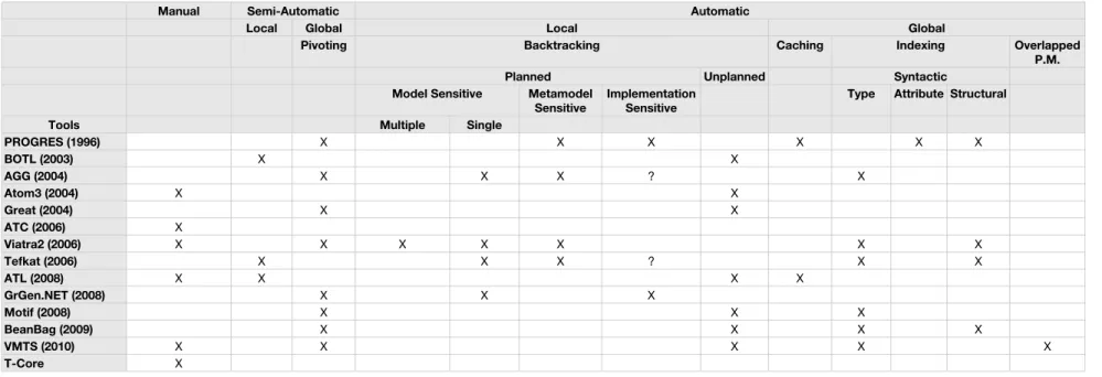
In this section, we present a summary of the state of the art tools and optimization tech-niques that they use. The tools we considered are: PROGRES [Zün96; Sch94], BOTL [BM03a; BM03b], AGG [Tae04; Rud00], Atom3 [LVA04], Great [BNBK07; VAS04], ATC [EPSR06], GrGen.NET [VBKG08;KG07;JBK10], Motif [SV08b;SV08a], BeanBag [XHZSTM09], VMTS [MML10;LLMC06] and T-Core [SV10].

Table 4.1 shows the results of our study. Since model transformation tools evolve very rapidly we have included the year next to the tool in which a paper was published concerning the tool’s internal mechanisms to perform pattern matching.

It is important to note that there are tools, such as AGG and GrGen(PSQL) that use a constraint satisfaction solver or a database management system as underlying pattern matching engine. In this sense, a pattern matching process relying on a CSP solver or a DBMS adopts the techniques employed in the underlying engine. CSP solvers perform backtracking search, use heuristics such as the first-fail principle, leverage information about the input model to determine the variables’ domain, perform forward checking and other optimization techniques [RN03]. That is why AGG is characterized as shown in Table4.1. DBMSs use query evaluation plans with sophisticated cost models that take into account statistics about the relations, indexes on their columns and the individual costs of operations [SKS10].

4.3.1 Discussion

(53)

4. PATTERNMATCHINGOPTIMIZATIONTECHNIQUES 4.3. State of the Art

to the CSP or DB domain also fit in the presented categorization. These facts allows us to compare the different pattern matching approaches and the tools that support them with-out having to consider other aspects such as their execution modes or if they perform a reduction to other domain.

In terms of performance, the imperative languages (see Czarnecki’s categorization [CH03]) such as ATC [EPSR06] or T-Core [SV10] or Java, despite not supporting many optimizations techniques, can be extremely fast. This is because the user can choose to directly code the optimizations. So it can apply virtually any optimization technique, as long as the language is expressive enough, which is generally true.

Naturally, those optimization techniques that depend on user intervention are the ones that contribute more to the performance but with an impact in the productivity and maintenance. On the other hand, those techniques that can be applied automatically, require less knowledge from the user and ease the creation and maintenance of the op-timized transformation specifications. As shown in Table4.1 tools that invest more in optimization tend to combine manual and automatic techniques.

(54)

P A T T E R N M A T C H IN G O P T IM IZ A T IO N T E C H N IQ U E S 4.3. State of the Ar t

Table 4.1: State of art tools and the pattern matching techniques in use.

Manual Semi-AutomaticSemi-Automatic AutomaticAutomatic

Local Global Local GlobalGlobal

Pivoting BacktrackingBacktrackingBacktracking Caching IndexingIndexingIndexing Overlapped P.M. Planned

Planned Unplanned SyntacticSyntacticSyntactic Model Sensitive

Model Sensitive Metamodel Sensitive

Implementation Sensitive

Type Attribute Structural

Tools PROGRES (1996) BOTL (2003) AGG (2004) Atom3 (2004) Great (2004) ATC (2006) Viatra2 (2006) Tefkat (2006) ATL (2008) GrGen.NET (2008) Motif (2008) BeanBag (2009) VMTS (2010) T-Core Multiple Single

X X X X X X

X X

X X X ? X

X X

X

X X X X X X X

X X X ? X X

X X X X

X X X

X X X X

X X X X X

X

(55)

5

Problem Definition

It is very clear by now that, in terms of performance, lower-level and imperative lan-guages are much better than high-level, declarative lanlan-guages. The problem is that, at a lower level of abstraction, transformations written in imperative languages are hard to create, read and maintain. However, only after transformations written at an high level of abstraction are shown to run fast enough, people will use them at industrial scales. Optimizations, and in particular those that target the pattern matching operation, play a key role.

This trade-off between abstraction and performance is not new, it is at least as old as the first high-level languages appeared.

5.1 Abstraction Penalty

There are plenty of sites, for example [Ful13] and [Att], that compare different program-ming languages with respect to their performance and, by observing one of the results taken from [Att] and shown in figure 5.1, it is clear that higher-level languages are typ-ically much slower than lower level ones. Another trivial conclusion is that compiled code, shown in red, runs a lot faster than interpreted code, in black.

(56)

5. PROBLEMDEFINITION 5.2. How to Avoid the Penalty

Figure 5.1: Programming languages benchmark on sudoku solving. Taken from [Att].

5.2 How to Avoid the Penalty

In order to understand what is the best way to mitigate the abstraction penalty, we have the study how General Purpose Programming Languages (GPLs) tackled that problem.

Assembly is a lot faster than C. Despite this, only a few people today code entirely in assembly. This is mainly because of three things: the raising complexity of software systems; the raising variety of processor architectures and, last but not least, performance optimization in the C compiler. There has been a lot of research in compiler optimization techniques and they have been applied to the C compiler [Aho08;SS08]. As a result, the C compiler has evolved to produce assembly code that is efficient enough to make coding directly in assembly a bad investment, i.e., it mitigated, for the most cases, the abstraction penalty.

(57)

5. PROBLEMDEFINITION 5.2. How to Avoid the Penalty

Figure 5.2 illustrates one particular representation that is used for many optimiza-tions: the Control Flow Graph (CFG). This representation supports many data-flow anal-yses that, once performed, result in optimizations such as reaching definitions, live vari-ables, available expressions [Aho08], etc. . . Note that we focused only on data flow anal-yses because they are machine independent optimization techniques. There are other, machine or architecture dependent but, since we are trying to solve the same (abstraction penalty) problem for model transformation languages which by nature promote platform independence, we are not interested in machine/platform dependent optimizations.

High L. Program

Low L. Program

Input Output

Intermediate Rep. Opt.

C

Assembly C. F. Graph

Processor

Figure 5.2: C Compilation Overview.

If we bring that architecture for the model transformation languages domain, we have something similar to what is illustrated in Figure5.3: an High-Level language, a process that translates the high-level representation of transformations to an intermediate one and then another that generates the final representation of the transformation. The high-level transformation language has to promote productivity and maintenance while the lower level language has to be fast. The intermediate representation has to promote anal-ysis and optimization.

DSLtrans [BLAFS11] which we presented in section 3.2, page14, is a good example of high level transformation language and, since it was developed internally, we have a much better understanding of its semantics than we have of other high-level transforma-tion languages.

Java, which we have shown to be really fast in the chart of Figure 3.5 (section 3.5), serves well enough to be our low-level transformation language. Other GPLs such as C or C++ have better performances but Java has a complete model manipulation library support from Eclipse Modelling Framework (EMF).

(58)

5. PROBLEMDEFINITION 5.3. General Requirements

High L. Transformation

Low L. Transformation

Input Model

Output Model

Output MM

conforms to

Intermediate Rep. Opt.

DSLTrans

Java ?

JVM Input

MM

Figure 5.3: High level model transformation language compilation overview.

5.3 General Requirements

As we have seen in Chapter 4, the most performance-critical operation is the pattern matching so it is only natural that this intermediate representation has to support natively the representation of this operation. It also has to allow for a fine-grained control over the how the operation will be executed. Off course, simplicity is always desirable when we want to achieve analyzability.

Since we are in the context of model transformations and model driven development, all the transformations in figure5.3should be model transformations and the intermedi-ate representation should be a full fledged language: with syntax and semantics.

(59)

6

Design

We need to find a language that links an high-level and productive transformation lan-guage to a low-level, fast one. In this thesis we will be using DSLTrans as the high-level language and Java as the low level language but we believe that the principles studied here are applicable to other high-level transformation languages and are independent of Java.

The main desirable traits of our language are: the ability to model the pattern match-ing operation and both syntactic and the semantic simplicity.

Figure 6.1 shows the general architecture of the solution to the abstraction penalty. The intermediate language is called TrNet (Transformation + Network) because it re-sembles a network of channels where input model elements and patterns flow and are transformed until they reach the output models. Analysis and optimizations operate as model transformations, processing the network, rearranging channels, defining parame-ters, etc. . .

In the following section we will the languages involved in this architecture, namely, the intermediate languages (TrNet), the high-level language (DSLTrans) and the tech-nologies used to design such languages.

A Framework for Efficient Model Transformations

Cláudio Ângelo Gonçalves Gomes