A Linear Interpolation-Based Algorithm for Path
Planning and Replanning on Girds
*
Changwen Zheng, Jiawei Cai, Huafei Yin
National Key Laboratory of Integrated Information System Technology Institute of Software, Chinese Academy of Sciences, Beijing, China
Email: [email protected]
Received April 5,2012; revised May 5, 2012; accepted May 20,2012
ABSTRACT
Field D* algorithm is widely used in mobile robot navigation since it can plan and replan any-angle paths through non- uniform cost grids. However, it still suffers from inefficiency and sub-optimality. In this article, a new linear interpola-tion-based planning and replanning algorithm, Update-Reducing Field D*, is proposed. It employs different approaches during initial planning and replanning respectively in order to reduce the number of updates of the rhs-values of vertices. Experiments have shown that Update-Reducing Field D* runs faster than Field D* and returns smoother and lower-cost paths.
Keywords: Field D* Algorithm; Path Planning and Replanning; Any-Angle Path; Linear Interpolation; Grid Cell
1. Introduction
In mobile robot navigation, path planning leads a robot from its initial location to some desired goal location. The two most popular techniques for path planning are deterministic algorithms and randomized algorithms [1]. Among deterministic algorithms, A* provides heuristic search in static, known environments [2]. LPA* com-bines heuristic search and incremental search [3]. D* Lite could replan in unknown environments efficiently [4].
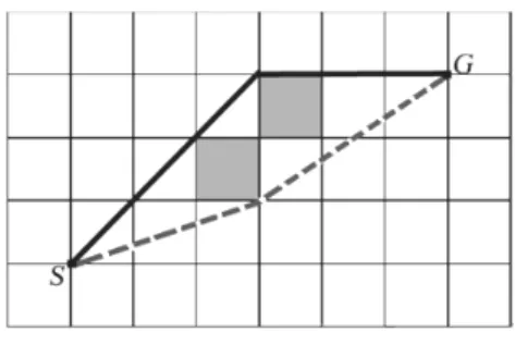
When provided with a grid-based representation of en-vironments, these algorithms are limited by the discrete set of possible headings between gird cells. For example, the eight-connected grids restrict the agent’s heading changes by multiples of π 4. As a result, the paths are suboptimal and unrealistic looking. To alleviate this problem, several methods for any-angle path planning have been investigated. A* PS uses post-smoothing to generate any-angle path [5]. But it does not always work as is showed in Figure 1 (The path returned by A* PS (in black line) is not the optimal path (in dash line) from S to
G). Basic Theta* algorithm and AP Theta* algorithm (Angle-Propagation Theta*) allow the parent of a node to be a node other than its local neighbor [6]. AA* (Accel-erated A*) can plan a shortest any angle paths fast [7]. However, these algorithm are only usable for uniform cost environments.
Based on D* Lite and linear interpolation, Field D*
could fast plan and replan any-angle path in grid envi-ronments, whatever the environment costs are known or partially-known, uniform or non-uniform [8]. Field D* is employed as the path replanner in a wide range of fielded robotic systems.
However, Field D* still suffers from two major draw-backs: 1) It plans and replans much slower than D* Lite. 2) The path returned by Field D* is not always the opti-mal solution. Motivated by these observations, a linear interpolation-based planning and replanning algorithm, Update-Reducing Field D* (URFD*), is proposed in this paper. It reduces the number of updates of the rhs-values so as to speed up the search. It also employs a method of post-smoothing to generate a lower-cost and smoother path. Besides, a heuristic with a variable factor according to the environments is used. As a result, the novel algo-rithm could efficiently produce a near-optimal path in non-uniform cost grids.
2. Linear Interpolation-Based Path Planning
2.1. The Idea of Field D*
Field D* stores the rhs-value, a one-step look ahead es-timate of the goal distance (by the goal distance of a ver-tex we mean the cost of an optimal path from this verver-tex to the goal). For vertex s it satisfies:
0, if
min , otherwise
goal
s nbrs s
s s rhs s
g s c s s
(1)
*This work was supported in part by the National Natural Science
Figure 1. Sub-Optimality of A* PS.
where sgoal is the goal vertex. denotes the set
of all neighboring vertices of s.
Nbrs s
g s is an estimate of goal distance of s. is the cost of a path be-tween
,c s s
s and s. In classical grid-based methods, it is assumed that s and s are two corner vertices and the path between s and s is a straight line. Field D* relaxes this assumption and takes any point along the boundary of a cell into consideration. To make it possible, Field D* makes an approximation that the path cost of any point sy
residing on the edge between two consecutive corner vertices s1 and s2 is a linear combination of g s
1 and
2
g s :
y
2 1
1g s yg s y g s (2)
where y is the distance from s1 to sy (assuming unit cells).
With the form of the optimal path in a unit cell, Field D* could compute and find the point to move by making
rhs s
d c s s, g s dv0, (3)
where v is the variable on which the path cost depends.
2.2. Differences and Inefficiency
A linear interpolation-based replanner performs differ-ently from a classical path replanner such as D* Lite, which leads to its inefficiency. To explain this, we define
g s as the cost of the optimal path from vertex s to the goal with respect to the linear interpolation assumption (so it is slightly different from the cost of the actual op-timal path). We call g s
(or rhs s
) is inaccurate when g s
(or rhs
s ) is not equal to g
s . Also we call g s
is more accurate than rhs s
when g s
is more close to g
s than rhs s
. g
s
satisfies:
0, if
min , otherwise.
goal
s nbrs s
s s g s
g s c s s
(4)
A linear interpolation-based replanner expands verti-ces in a different way from D* Lite. With a consistent heuristic, a locally overconsistent vertex (whose g-value is lager than rhs-value) becomes locally consistent (the
g-value equals rhs-value) after selected for expansion and then remains locally consistent until edge cost changes
are detected in D* Lite. It implies that D* Lite expands any locally overconsistent vertex at most once. However, a linear interpolation-based replanner tends to expand a locally overconsistent vertex for many times. Besides, the key values (denoting the priorities of vertices in the priority queue) of the vertices selected for expansion are monotonically nondecreasing over time in D* Lite, while it is not naturally the case in a linear interpolation-based replanner. This can be explained as follows: For some vertex s, the computation of its rhs-value is based on the
g-value of one neighboring vertex in D* Lite, but the
g-values of two neighboring vertices in a linear interpo-lation-based replanner. During the planning and replan-ning process, it is common that at least one of the two neighboring vertices has an inaccurate rhs-value. Relied upon them, s will get an inaccurate rhs-value. And the vertices relied upon s will also be affected, and so on. It is the reason that a linear interpolation-based replanner updates the rhs-values of vertices repeatedly to their final results. Such a phenomenon is easily observed particu-larly in environment consisting mainly of free space since the g-value of a vertex is very close to those of its neighbors in free space.
After the cost field created, path extraction for linear interpolation-based replanners is also different from that for D* Lite. When backpointers are not recorded, D* Lite can trace back a lowest-cost path from sstart to sgoal by
always moving from the current vertex s, starting at sstart,
to any neighbor s that minimizes c s s
,
g s
untilsgoal is reached. So the optimality of the result depends on
the accuracy of g s
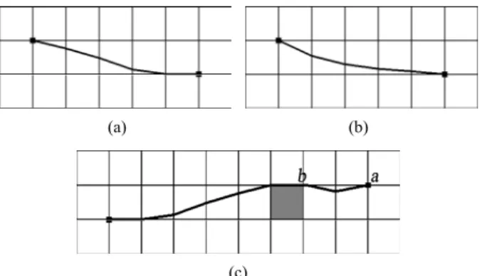
. But in a linear interpolation- based replanner the g-values are not the goal distances exactly, resulting in the sub-optimality of paths.From the discussion above, we can see that there exist two major drawbacks of Field D*: 1) It plans and replans much slower than D* Lite, especially in the environ-ments consisting mainly of free space. 2) The solution path is not the optimal solution. Figure 2 shows the sec-ond problem. The path returned by Field D* has unnec-essary heading changes even if no obstacle exists (see Figure 2(a)). To extract a smoother path, [9] gives a gra-dient interpolation method. The result is showed in Fig-ure 2(b), from which we can see that the unnecessary heading changes still exit. Obstacles can also make the interpolation assumption break down so that affects the quality of extracted paths. To alleviate it, [8] uses a one- step look ahead mechanism. But this method checks very limited steps so that cannot avoid generating a pathologic path between vertices a and b in Figure 2(c).
3. Update-Reducing Field D*
3.1. Basic Idea
(a) (b)
(c)
Figure 2. Paths returned by interpolation methods.
depends heavily on the number of updates of the rhs- values of vertices, the key to high efficiency of our algo-rithm is reducing the number of updates. We use the fringe vertices to refer to the vertices on the fringe of the expanded vertices during initial planning. The fringe vertices have not been expanded yet so that their g-values are not computed (namely infinite), leading the rhs-val- ues computed by the g-values of the fringe vertices to inaccuracy. Then the inaccurate rhs-values along with the infinite g-values affect next vertex expansions. This is the main source of the repeated updates of rhs-values. Note that most of the fringe vertices are just locally over- consistent vertices during initial planning, as is showed in Figure 3. (The locally consistent vertices (in light grey), which have been expanded at least once, are almost sur-rounded by the locally overconsistent vertices (in dark grey). Vertices in black are obstacles.) The rhs-values of locally overconsistent vertices are better informed and thus more accurate than the g-values. So when it is a locally overconsistent vertex, we can use the rhs-value instead of the g-value to make the computation more close to the
g*-value. When it is a locally consistent vertex, we can also use the rhs-value because it equals the g-value and thus could get a result at least no poorer than that com-puted by the g-value.
During replanning, if we only encounter cell cost de-creases the approach above is still useful. However, when locally underconsistent vertices (whose g-values are smaller than rhs-values) appear, this approach tends to make the algorithm less efficient and even incomplete. It could be explained as follows: When the rhs-value of a vertex becomes larger due to edge cost increases, the old
rhs-value is out of date and thus to be abandoned. How-ever, the algorithm does not distinguish between the old and the new so that it is possible for the old rhs-value to be used to compute the rhs-value of another vertex, re-sulting in “false” relation between these two vertices. For example, there exist two vertices a and b. After initial planning, g(a), rhs(a) and g(b) are all infinite, rhs(b) is 50. Then rhs(a) and rhs(b) are updated due to cell cost increases. When rhs(a) is recomputed, old rhs(b) (namely
Figure 3. A snapshot during initial planning of Field D*.
50) is used. Then rhs(b) is updated to a new value of 64. Thus, the computation of rhs(a) seems to rely on rhs(b) but in fact this relation possibly dose not exist. Further-more the wrong rhs(a) leads to a priority error of a (g(a) is infinite so that does not affect the key value), which possibly makes a expand while b can never be expanded again. Thus the “false” relation has no chance to be cor-rected, resulting in the incompleteness of the algorithm.
In order to reduce the updates of the rhs-values during replanning, we use a technique similar to which Delayed D* used to speed up D* Lite [10], that is, delaying the processing of locally underconsistent vertices.
During path extraction, A* search, which depends on the accuracy of heuristic less heavily than greedy search does, could avoid errors caused by obstacles (see Figure 2(c)). However, based on the linear approximation, A* search still cannot ensure an optimal path even if no ob-stacles exist (see Figure 2(b)). And greedy search needs to be kept for checking solution paths for any loops. Note that the limitation of post-smoothing showed in Figure 1 can be overcome if it is already an any-angle path before smoothing.
Combined with the methods above, Update-Reducing Field D* (URFD*) is a modified version of Field D*. It redefines the rhs-values (denoted by rhs’-values to be distinguished from the original) as
0 i
min , otherwise
f goal
s nbrs s
s s rhs s
rhs s c s s
(5) where notation follows from (1). URFD* calculates the
rhs-values of vertices according to (5) during initial plan-ning. During replanning it calculates the rhs-values ac-cording to (1), which is similar to Field D*, and delays the propagation of cost increases. It checks the consis-tency of a path in every path extraction and ends with a post-smoothing step.
3.2. Algorithm Description
( )
01. return [min( ( ), ( )) ( , ); min( ( ), ( ))];
( )
02. for all ( ) ( ) ; 03. ( ) 0; ; ; 04. Insert( , , Key(
start
goal
goal go
s
g s rhs s h s s g s rhs s
s
s S rhs s g s
rhs s U raise false
U s s
Key Initialize )); ( , , , )
05. Use and to compute ( );
( ) 06. if ( ( ) ( )) 07. if ( ) Remove( , ); 08. Insert( , , Key( )); 09. else
al
a b
a b
s s s cost
cost s cost s rhs s
s g s rhs s
s U U s
U s s
ComputeCost
UpdateState
( ) ( )
if ( ( ) ( ) AND ) Remove( , );
( ) 10. if ( ( ) ( )) 11. if ( ) Remove( , ); 12. Insert( , , Key( ));
13. else if ( ( ) ( ) AND ) Remove( , );
g s rhs s s U U s
s g s rhs s
s U U s
U s s
g s rhs s s U U s
UpdateStateLower Co
( ', ") ( ) ( ', ") ( )
( ) 14. if ( )
15. if (it is inital planning) ( ) min ComputeCost( , ', ", ); 16. else ( ) min ComputeCost( , ', ", );
goal
s s connbrs s
s s connbrs s s
s s
rhs s s s s rhs
rhs s s s s g
mputeState Comp ()
17. while(min (Key( )) Key( )) OR ( ) ( )) 18. .Top();
19. if ( ( ) ( )) 20. ( ); 21. Remove( , ); 22.
s U s sstart rhs sstart g sstart
s U
g s rhs s g s rhs s U s uteShortestPath
for all ' ( )
23. ComputeState( '); UpdateStateLower( '); 24. else
25. ( ) ;
26. for all ' ( ) { } 27. ComputeS
s nbrs s
s s
g s
s nbrs s s
' ( )
tate( '); UpdateState( ');
()
28. ; ; 0; ;
29. while( AND AND )
30. arg min ( ( start
goal
s succ s
s s
raise false s s ctr loop false
s s loop false ctr maxsteps
x c
FindRaiseStatesOnPath
, ') ( ')); 31. for all ' ( )
32. if ( ' is locally inconsistent AND ' has never been added into with local underconsistency during this replann
c s s g s s vicinity s
s s
U
ing episode) 33. ComputeState( '); UpdateState( '); ;
34. if ( is visited before ; 35 ; ;
() 36. Initialize(); 37. Com
s s raise true
s loop true
s x ctr
Main ) puteShortestPath(); 38. Path extraction; 39. Post-Smoothing; 40. forever
41 Wait for changes in cell costs; 42. for all cells with changed costs 43. for each
x
state on a corner of
44. ComputeState( ); UpdateStateLower( ); 45. ComputeState( ); UpdateState( ); 46. ComputeShortestPath(); F
start start
s x
s s
s s
indRaiseStatesOnPath();. 47. while( )
48. ComputeShortestPath(); FindRaiseStatesOnPath();. 49. Post-Smoothing;
raise
Figure 4. The update-reducing Field D* algorithm.
During initial planning, URFD* calls ComputeShortest-Path() to expand vertices. ComputeCost() calculates the
rhs-value in a way similar to the interpolation-based path cost calculation in Field D*, but every vertex uses rhs-
values, instead of g-values, of its neighbors. ComputeS-tate() then computes the rhs-values according to (5) (line 15). During replanning, ComputeState() calls Compute-Cost() to compute the rhs-values according to (1) (line 16). The rhs-values of the start vertex and every vertex immediately affected by the changed edge costs are up-dated, but only the locally inconsistent start vertex and locally overconsistent vertices are inserted into priority queue U for expansion (lines 42 - 45). Then FindRaiseS-tatesOnPath() (FRSOP) is called. FROSP checks whether locally underconsistent vertices are in the vicinity of the node. All the unprocessed locally underconsistent verti-ces that are adjacent to this node will be added into prior-ity queue U (lines 31 - 33). Here vicinity(s) refers to the set of all corner vertices in the vicinity of node s (s is included). When the number of nodes exceeds the given limit maxsteps, or a loop is found, which indicates a po-tential failure of path extraction, FRSOP stops the ex-traction to expand locally underconsistent vertices in priority queue U. After path extraction, the solution path is post-processed by a smoothing step. (lines 39, 49). Given two cell boundary nodes along the path, the post- smoothing replaces the solution path between these two nodes with a straight line path if the latter is less costly. It is done with cell boundary nodes along the solution path iteratively. However, some small techniques are used to avoid a large amount of computation: 1) It only performs a single iteration. 2) It only smoothes the path between cell corners because necessary and sharp heading changes usually occur on them. 3) Before smoothing a path be-tween two cell corners, it checks whether the costs of all grid cells that the original path is through are all same. If they are, the original path is kept.
4. Experimental Results
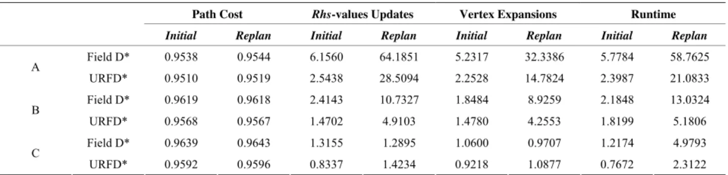
Table 1. Performance comparison among URFD*, Field D* and Delayed D* in three kinds of environments.
Path Cost Rhs-values Updates Vertex Expansions Runtime
Initial Replan Initial Replan Initial Replan Initial Replan
Field D* 0.9538 0.9544 6.1560 64.1851 5.2317 32.3386 5.7784 58.7625 A
URFD* 0.9510 0.9519 2.5438 28.5094 2.2528 14.7824 2.3987 21.0833
Field D* 0.9619 0.9618 2.4143 10.7327 1.8484 8.9259 2.1848 13.0324
B
URFD* 0.9568 0.9567 1.4702 4.9103 1.4780 4.2553 1.8199 5.1806
Field D* 0.9639 0.9643 1.3155 1.2895 1.0600 0.9707 1.2174 4.9793
C
URFD* 0.9592 0.9596 0.8337 1.4234 0.9218 1.0877 0.7672 2.3122
path. We use the weighted heuristic, which is described in the previous section, for URFD* and Field D*.
We selected the results in three kinds of environments (A: uniform cost grids with 10% obstacle cells. B: uni-form cost grids with 30% obstacle cells. C: non-uniuni-form cost grids with 50% free space cells) and showed them in Table 1. Four performance measures were used here: the path cost, the total number of rhs-value updates (that is, updates of the rhs-values), the total number of vertex ex- pansions (updates of the g-values) and the runtime. Each value is a ratio of a performance measure of URFD* (or Field D*) to that of Delayed D* averaged over initial planning (or replanning) episodes. Note that in environ-ments with more free space the runtimes of initial plan-ning and replanplan-ning of Field D* drastically increased while those of URFD* increased much more stably. The performance in environments C shows the possibility that the number of updates of the rhs-values during replan-ning could be slightly larger than that of Field D* in some scenarios. However, since the number of vertices in the priority queue is limited by selectively processing locally underconsistent vertices, making the priority queue operations less expensive, the runtime of URFD* is still shorter than that of Field D* in those scenarios.
5. Conclusion
We present URFD*, a linear interpolation-based algo-rithm that plans and replans any-angle paths in dynamic environments with uniform and non-uniform cost grids. It makes efforts in the reduction of updates of the rhs- values, which contributes to the gain in efficiency. The solution paths returned by URFD* are smooth and near- optimal. As opposed to Field D*, it performs faster plan-ning and replanplan-ning and returns a path with lower cost and fewer heading changes. However, URFD* is not optimal either due to the linear interpolation assumption.
REFERENCES
[1] D. Ferguson, M. Likhachev and A. Stentz, “A Guide to
Heuristic-Based Path Planning,” Proceedings of the Work- shop on Planning under Uncertainty for Autonomous Sys- tems at the International Conference on Automated Plan- ning and Scheduling, Monterey, 5-10 June 2005, pp. 9- 18.
[2] P. Hart, N. Nilsson and B. Raphael, “A Formal Basis for
the Heuristic Determination of Minimum Cost Paths,”
IEEE Transactions on Systems Science and Cybernetics, 1968, Vol. 4, No. 2, pp. 100-107.
[3] S. Koenig, M. Likhachev and D. Furcy, “Lifelong Plan-
ning A*,” Artificial Intelligence Journal, Vol. 155, No. 1-2, 2004, pp. 93-146.
[4] S. Koenig and M. Likhachev, “Improved Fast Replanning
for Robot Navigation in Unknown Terrain,” Proceedings
of the IEEE International Conference on Robotics and Automation (ICRA 2002), Washington, 11-15 May 2002, pp. 968-975.
[5] A. Botea, M. Müller and J. Schaeffer, “Near Optimal
Hierarchical Path-Finding,” Journal of Game
Develop-ment, 2004, Vol. 1, No. 1, pp. 1-22.
[6] A. Nash, K. Daniel, S. Koenig and A. Felner, “Theta*:
Any-Angle Path Planning on Grids,” Proceedings of the
National Conference on Artificial Intelligence, 22-26 July 2007, Vancouver, pp. 1177-1183.
[7] D. Šišlák, P. Volf and M. Pěchouček, “Accelerated A*
Path Planning,” Springer-Verlag, Berlin, 2009.
[8] D. Ferguson and A. Stentz, “The Field D* Algorithm for
Improved Path Planning and Replanning in Uniform and Non-Uniform Cost Environments,” Technical Report, Car- negie Mellon University, Pittsburgh, 2005.
[9] M. W. Otte and G. Grudic, “Extracting Paths from Fields
Built with Linear Interpolation,” IEEE/RSJ International Conference on Intelligent Robots and Systems, St. Louis, 10-15 October 2009, pp. 4406-4413.
[10] D. Ferguson and A. Stentz, “The Delayed D* Algorithm
for Efficient Path Replanning,” Proceedings of the IEEE