Application for photogrammetry of organisms

(1)

Department of Information Science and Technology

Application for Photogrammetry of Organisms

Francisco Faria Aleixo

Dissertation submitted as partial fulfillment of the requirements for the degree of

Master in Computer Engineering

Supervisor:

PhD Luís Eduardo de Pinho Ducla Soares, Assistant Professor, ISCTE-IUL

Co-supervisor:

PhD Paulo Jorge Lourenço Nunes, Assistant Professor, ISCTE-IUL

External co-supervisor:

PhD Rui Conde de Araújo Brito Prieto da Silva, Research Associate, MARE – Centro de Ciências do Mar e do Ambiente

(2)

(3)

Application for Photogrammetry of Organisms

i

Acknowledgments

I would like to express my gratitude to my institution supervisors, Professor Luís Soares and Professor Paulo Nunes for their great discussions, support, motivation and guidance throughout this process, which proved to be very important. Their constant positive outlook and good mood made the whole process a lot more enjoyable. I also wanted to note their availability, even in unreasonable time frames.

I’d also like to give a special thanks to supervisor Doctor Rui Prieto, who was responsible not only for the topic of the present work but was also a major influence throughout the development and writing of this work. His great help, patience, availability and enthusiasm were a big motivation throughout this process and absolutely invaluable. Finally, I would like to deeply thank my family and friends that supported and pushed me throughout this phase. They were equally important and invaluable.

This thesis was supported by research project WATCH IT - Whale watching effects on sperm whales - disturbance assessment towards a sustainable ecotourism (ACORES-01-0145-FEDER-000057), co-funded by AÇORES 2020, through the FEDER fund from the European Union.

(4)

(5)

iii

Resumo

Fotogrametria em câmera única é um procedimento bem estabelecido para recolher dados quantitativos de objectos através de fotografias. Em biologia, fotogrametria é frequentemente aplicada no contexto de estudos morfométricos, focando-se no estudo comparativo de formas e organismos. Nos estudos morfométricos são utilizados dois tipos de aplicação fotogramétrica: fotogrametria 2D, onde são utilizadas medidas de distância e ângulo para quantitativamente descrever atributos de um objecto, e fotogrametria 3D, onde são utilizadas coordenadas de referência de forma a reconstruir a verdadeira forma de um objeto. Apesar da existência de uma elevada variedade de software no contexto de fotogrametria 3D, a variedade de software concebida especificamente para a a aplicação de fotogrametria 2D é ainda muito reduzida. Consequentemente, é comum observar estudos onde fotogrametria 2D é utilizada através da aquisição manual de medidas a partir de imagens, que posteriormente necessitam de ser escaladas para um sistema apropriado de medida. Este processo de várias etapas é frequentemente moroso e requer a aplicação de diferentes programas de software. Além de ser moroso, é também susceptível a erros, dada a natureza manual na aquisição de dados. O presente trabalho visou abordar os problemas descritos através da implementação de um novo software multiplataforma capaz de integrar e agilizar o processo de fotogrametria presentes em estudos que requerem fotogrametria 2D. Resultados preliminares demonstram um decréscimo de 45% em tempo de processamento na utilização do software desenvolvido no âmbito deste trabalho quando comparado a uma metodologia concorrente. Limitações existentes e trabalho futuro são discutidos.

Palavras-Chave: Fotogrametria, Morfometria, Software, Biologia, Medição, Fotografia, Aplicação.

(6)

(7)

v

Abstract

Single-camera photogrammetry is a well-established procedure to retrieve quantitative information from objects using photography. In biological sciences, photogrammetry is often applied to aid in morphometry studies, focusing on the comparative study of shapes and organisms. Two types of photogrammetry are used in morphometric studies: 2D photogrammetry, where distance and angle measurements are used to quantitatively describe attributes of an object, and 3D photogrammetry, where data on landmark coordinates are used to reconstruct an object true shape. Although there are excellent software tools for 3D photogrammetry available, software specifically designed to aid in the somewhat simpler 2D photogrammetry are lacking. Therefore, most studies applying 2D photogrammetry, still rely on manual acquisition of measurements from pictures, that must then be scaled to an appropriate measuring system. This is often a laborious multi-step process, on most cases utilizing diverse software to complete different tasks. In addition to being time-consuming, it is also error-prone since measurement recording is often made manually. The present work aimed at tackling those issues by implementing a new cross-platform software able to integrate and streamline the photogrammetry workflow usually applied in 2D photogrammetry studies. Results from a preliminary study show a decrease of 45% in processing time when using the software developed in the scope of this work in comparison with a competing methodology. Existing limitations and future work towards improved versions of the software are discussed.

Keywords: Photogrammetry, Morphometry, Software, Biology, Measurement, Photography, Application.

(8)

(9)

Application for Photogrammetry of Organisms vii

List of tables

Table 1 - Quantitative results of time taken to perform two different steps of the

(14)

(15)

xiii

List of figures

Figure 1 – An aerial photograph of a full whale’s body (left) and a photograph taken

from a boat photoshoot (right) (Azores Whale Lab, n.d.). ... 10

Figure 2 - Types of typical radial distortions. Barrel distortion (left), pincushion distortion (middle) and mustache distortion (right) (WolfWings, 2010). ... 12

Figure 3 – A set of photographs of a planar calibration pattern at different angles to be used for camera calibration. ... 13

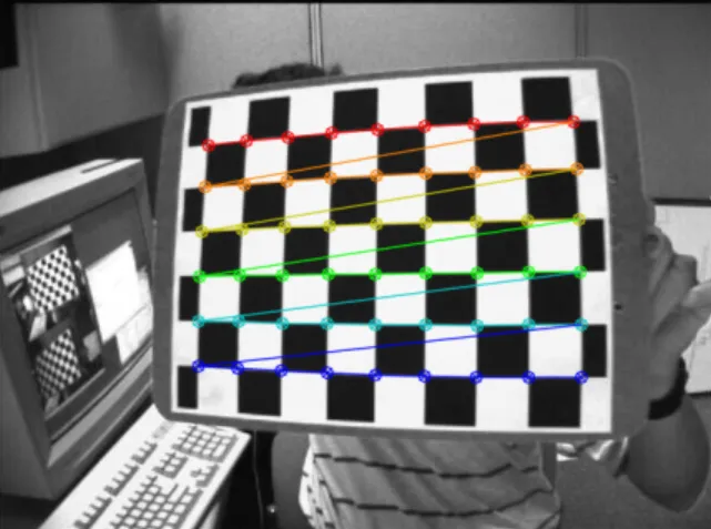
Figure 4 – Representation of detected corners on a chessboard pattern. ... 15

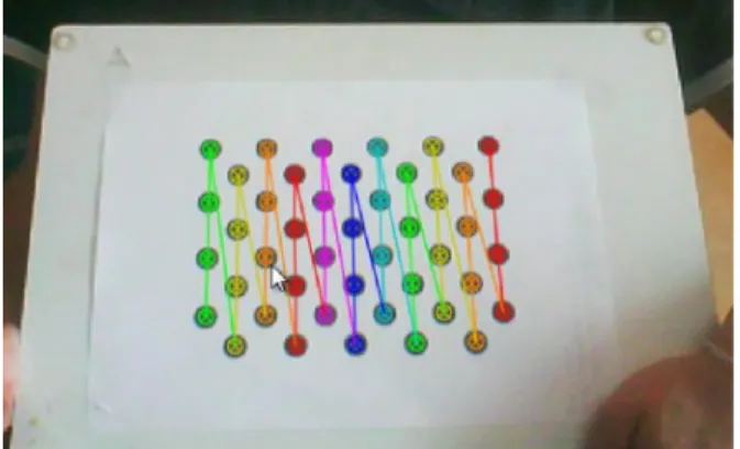
Figure 5 – Representation of found circle centers on a circle grid pattern. ... 16

Figure 6 – Representation of found corners on a deltille grid pattern (Ha et al., 2017). 17 Figure 7 – Original image (left) and the “undistorted” image using the regular Pinhole model (right). ... 21

Figure 8 – Original image (left) and the corrected image using the Kannala model (right). ... 21

Figure 9 – Basic structure of a JPEG compressed file (JEITA, 2002). ... 24

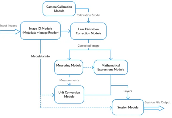
Figure 10 – Overview of module interaction. ... 29

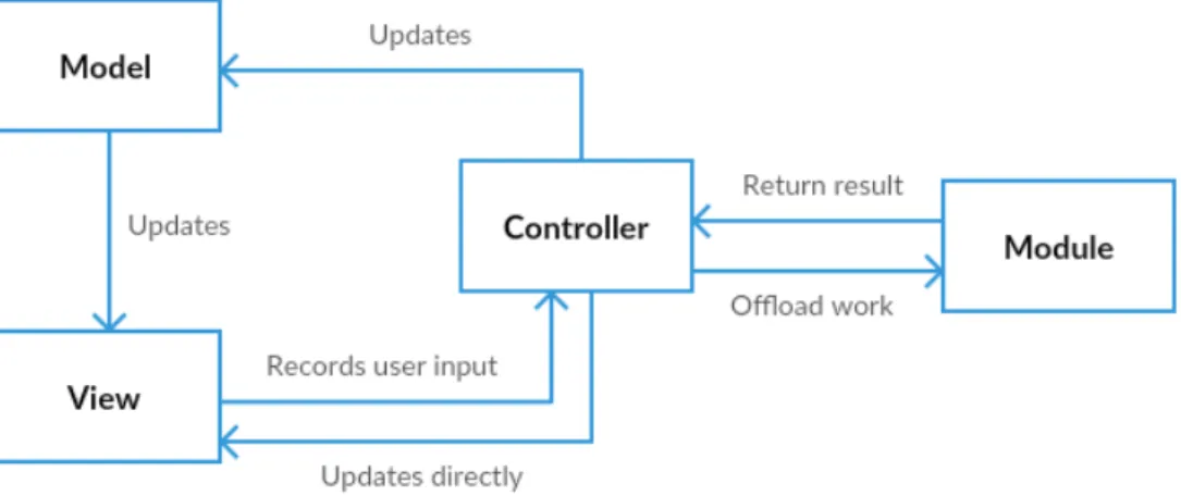
Figure 11 - Overview of the adopted MVC related architecture. ... 30

Figure 12 – The different components of the main screen represented by different colors. ... 31

Figure 13 – Overview of the calibration module architecture. ... 33

Figure 14 – The different delimited components of the calibration screen. ... 34

Figure 15 – Calibration configuration dialog. ... 35

Figure 16 - Undistort dialog. ... 38

Figure 17 – Example of two perpendicular measuring lines. ... 39

Figure 18 – Reference scaling dialog example. ... 40

Figure 19 – Distance scaling dialog example. ... 41

Figure 20 – Example of resulting centimeter conversion. ... 41

Figure 21 – Example of setting mathematical expression and attributing variable value. ... 42

Figure 22 – Example of a resulting expression value in the layer list. ... 43

Figure 23 – Setting a metadata tag to be exported. If set to export, the tag will have a blue ‘e’ preceding it. Whole metadata directories, such as Exif can be set to export. ... 46

Figure 24 – Experiment extracted measurements: one for animal length, three for width. ... 49

(16)

(17)

xv

List of abbreviations and acronyms

APP – Application

BMP – Bitmap (image file)

Exif – Exchangeable Image File Format GC – Garbage Collector

GIF – Graphics Interchange Format

GIMP - GNU Image Manipulation Program IFD – Image File Directories

I/O – Input/Output

ISO – International Organization for Standardization

JEIDA – Japan Electronic Industries Development Association JFIF – JPEG File Interchange Format

JPEG – Joint Photographic Experts Group

MARE – Marine and Environmental Sciences Centre MVC – Model-view-controller

MVP – Model-view-presenter MVVM – Model-view-viewmodel PC – Personal Computer

PNG – Portable Network Graphics RDF – Resource Description Framework TIFF – Tagged Image File Format XMP – Extensible Metadata Platform XML – Extensible Markup Language

(18)

(19)

Introduction

1

Chapter 1 – Introduction

1.1. Context

The quantitative analysis of size and shape is essential for several branches of science, and comprises a set of measuring and analytical methods, collectively grouped in a field referred as Morphometrics (Elewa, 2010; Reyment, 1996, 2010; Rohlf, 1990). The origin of the term Morphometrics is attributed to Blackith (1957), however the field started being developed much earlier, with pioneering works being published by the end of the 19th_{century (e.g., Weldon, 1890). Morphometrics is deeply intertwined with biological}

studies on phylogeny, ecology, and physiology, but it also progressively found applications in geomorphology, medicine, anthropology, behavioral sciences and forensics (Elewa, 2010). Morphometric methods allow the description and comparison of shapes of organisms or objects in a standardized manner, allowing for investigations on variability due to distribution, development stage, gender, genetic and environmental effects, among others.

Traditional morphometrics has made use of (and in fact was partially on the basis for the development of) multivariate statistical methods, such as principal component analysis (PCA), cluster analysis, and similar methods, over data in the form of matrices of distance and angle measurements (Jensen, 2003; Rohlf & Marcus, 1993). This approach is still very useful for a plethora of applications; however, it has the drawback of not allowing the reconstruction of the original form from the measurements that are usually taken. Beginning in the mid-1980’s, in part because of growing scientific needs, but also due to the unprecedented progress of computational power, a ‘revolution’ in Morphometrics took place, through new methods that enabled defining shape as a set of distances among landmark coordinates and the geometric information about their relative positions (Jensen, 2003; Rohlf & Marcus, 1993). These new methods utilizing landmark and outline analyses have been termed Geometric Morphometrics to differentiate from the traditional Morphometrics methods that were already well established (Adams, Rohlf, & Slice, 2004). The present work focuses in techniques related to the former case and, as such, hereon all mentions to Morphometrics and morphometry methods relate to traditional Morphometrics, unless otherwise stated.

(20)

Introduction

2 1.2. Motivation and relevance

Despite the dramatic evolution seen in the field of Morphometrics, the process of recording morphometric data is often resource- and labor-intensive and can also be time-consuming when no appropriate tools are available (Adams, Rohlf, & Slice, 2013). Morphometry studies often involve the collection of multiple measurements from a representative sample of individuals in a population, which normally translates in at least few, to tens or even hundred thousands measurements taken in the course of a single study (Kocovsky, Adams, & Bronte, 2009; Rising & Somers, 1989).

Semi-automatic measuring equipment, linked to a computer, handheld PC, or with inboard processing capability, started being introduced in the early 1980’s to side-step the laborious and error-prone process of transcribing measurement hand notes to a digital database (e.g., Morizur, Ogor, & Lespagnol, 1994; Sprules, Holtby, & Griggs, 1981). However, these equipments rely in the manipulation of the object or organism being measured, which is not always practical, or overall feasible. For example, capturing and measuring many marine organisms is often impossible due to logistical constraints related to the environment in which they live or to the sheer size of the animals (large whales being a paradigmatic example). Similarly, very small (microscopic) organisms and objects cannot be easily manipulated in order to obtain measurements. For those cases, other methods of measurement must be employed, one of the most prominent being photogrammetry.

Photogrammetry is a technique that makes use of photography to obtain measurements of physical objects, by scaling measurements taken directly on the photographic reproduction of an object, using basic geometric principles. Using the information stored in a photography to obtain measurements of objects was first proposed by François Arago, when discussing the applications of the (then) new daguerreotype technology (an early photographic process), during an address to the French Academy of Sciences (Arago, 1839). Since then, photogrammetry has become a well-established measuring procedure, being widely used in geodesy, but also in other fields ranging from cell biology to astrophysics (Kraus, 2011; Luhmann, Robson, Kyle, & Harley, 2006).

Photogrammetry techniques are diverse but the most common fall in two broad categories, aerial and terrestrial, which in turn can be either, close- (when camera to object distance is less than around 300 meters) or long-range (when camera to object distance is more than around 300 meters) (Luhmann et al., 2006). Micro photogrammetry (sometimes also termed ‘macro photogrammetry’ due to the type of lenses used) is a

(21)

Introduction

3

special case of close-range photogrammetry, when the image scale >1 (Luhmann et al., 2006).

In the context of biological research, when photogrammetric techniques are used they tend to belong overwhelmingly to close-range photogrammetry and the basic procedure can be broken down in to three generalized steps:

1. Gathering proper and relevant photographs of the body structures meant to be measured;

2. Measuring the relevant body structures on the photographs, using either analogic or digital tools with appropriate resolution;

3. Scaling from image units to a relevant measuring system, such as metric or imperial, from known scaling equations.

As with direct morphometry, where measurements are taken directly from the specimens, in photogrammetry-aided studies making and recording measurements is usually also labor-intensive when done manually. Unfortunately, despite advances in automation of measurement acquisition in close-range photogrammetry, there is a number of situations where such automation is not possible, and the use of manual measurement is needed.

As mentioned earlier for direct morphometry, not only taking thousands of manual measurements from pictures can become one of the most time-consuming parts of any morphometry study, it also usually implies transcribing those measurements to a digital database, which adds to the lengthy process of data acquisition and preparation prior to analysis. Additionally, data errors from transcription to database can compromise data quality (W. Kim, Choi, Hong, Kim, & Lee, 2003). In fact, data is usually corrupted during data entry by humans, either due to typographical errors or erroneous interpretation of written notes, and is still one of the most common sources of data-quality issues in databases (Hellerstein, 2008).

It becomes clear that photogrammetry-aided morphometry studies can benefit from software that aid in capturing and transcribing data in an automatic or semi-automatic way. However, it is often the case that existing software solutions are either too expensive or are not appropriate for having been designed for a totally different application and/or not contemplating all steps in a workflow. Well designed software should aid during several stages of the workflow, decreasing both processing time and human error by

(22)

Introduction

4

reducing complexity and automating data transcription (Gentleman et al., 2004; Hellerstein, 2008).

The present work aimed at creating a software package to tackle those goals while ensuring enough flexibility to be useful in a wide-range of morphometric studies. Researchers from the Azores Whale Lab, associated with the Marine and Environmental Sciences Centre (MARE), helped with the development of the software by iteratively testing it and by providing feedback about the user experience.

Morphometric data from whales is essential for several lines of research developed at the Azores Whale Lab. Nevertheless, due to their size, capturing whales is unfeasible and, consequently, photogrammetry is a preferred way to obtain relevant morphological data from different individuals. Photogrammetry provides additional benefits, such as larger sample sizes due to cost-effectiveness, increasement of safety to the researchers, and less disturbance to the whales (J. W. Durban, Fearnbach, Barrett-Lennard, Perryman, & Leroi, 2015).

1.3.Investigation objectives

The general objective is to explore, formulate and implement a solution to simplify and expedite the retrieval of morphometric data of animals from photographs with results comparable to current solutions. The proposed and implemented solution, therefore, must be an easier and faster way to retrieve morphometric data than current procedures. It will be compared with the current photogrammetry procedure employed by the researchers at Azores Whale Lab.

It is important to note that although direct comparisons will be made against the Azores Whale Lab photogrammetry procedure, the solution should still be general enough to be used in different photogrammetry contexts and applications. It would also be ideal if the solution is cross-platform, or at least capable of easily being ported into other platforms.

1.4.Methodology

As mentioned above, the solution proposed in the scope of this work was developed with the cooperation of researchers at Azores Whale Lab and direct contact with them was crucial, namely in gathering feedback about design choices, usability and bugs. For development, a Kanban based agile methodology was used (Sugimori, Kusunoki, Cho, &

(23)

Introduction

5

Uchikawa, 1977), where continuous releases and adjustments were made based on feedback. Ideally, this would span a one- or two-week cycle of development to testing, but in reality, it was not as regular and it varied from one week to one month.

The development releases of the program were published on the GitHub platform. There were several reasons for this, namely:

- It allows public discussion and feedback through the use of the issues feature; - It provides a way to label each issue which provides additional organization.

Labels such as ‘bug’, ‘duplicate’, ‘enhancement’ and priority related labels were created and used to help organize and prioritize the development work;

- It provides an easy and intuitive way to track the progress of each issue, through the use of a Kanban board, where each issue can be seen akin to a ticket;

- It provides a wiki platform, where it is possible to explain and detail how the program works and how it can best be used;

- It provides a way to publish and track different releases of the program.

Final analysis and comparison in usability and usage time between current solutions and the new solution was also done with the cooperation of researchers at the Azores Whale Lab. The comparison details, including the data collection process, results and limitations is further discussed in Chapter 4.

1.5. Dissertation structure and organization

This document is organized in five different chapters describing the different phases until its conclusion.

The first chapter introduces the dissertation theme, the motivation, its objectives and the document structure.

The second chapter expands the relevance, current solutions and theoretical framework of the photogrammetry procedure and each of its steps.

The third chapter describes in detail the proposal and implementation of an integrated system capable of solving the presented challenges that were identified in previous chapters.

The fourth chapter presents a comparison between previous solutions and the proposed system through the analysis of quantitative and qualitative results.

(24)

Introduction

6

The fifth and last chapter presents the study conclusions, recommendations, limitations, possible contributions to the scientific community and future research.

(25)

Photogrammetry theoretical framework

7

Chapter 2 – Photogrammetry theoretical framework

2.1. Introduction

This chapter is composed of five Sections and describes the theoretical framework behind the photogrammetry process and its steps. The first Section introduces and describes the chapter structure.

The second Section explores the different applications of photogrammetry, as well as its relevance to biological sciences. It further delineates the general process of photogrammetry and describes a specific example within the field that will be used as reference throughout this work. Finally, relevant software and existing solutions are presented.

The third, fourth and fifth Sections describe the relevance and theoretical framework of relevant steps in the photogrammetry process noted in the second Section. The third Section relates to the specific step of camera calibration and image distortion correction. The fourth Section relates to image metadata extraction. Finally, the fifth Section relates to measurement acquisition and unit conversion, also referred as scaling.

2.2. Computer-aided photogrammetry 2.2.1. Relevance and current solutions

As has already been pointed in Chapter 1, photogrammetry has a wide range of applications, with examples in many fields, including microscopy (e.g., Boyde & Ross, 1975), archaeology and paleontology (e.g., Fussell, 1982; Mallison & Wings, 2014), anthropology and forensics (e.g., Grip, Grip, & Morrison, 2000; Milliet, Delémont, & Margot, 2014), astronomy (e.g., Googe, Eichhorn, & Luckac, 1970), industry (e.g., Fraser & Brown, 1986), geodesy (e.g., Kraus, 2011), among many others.

The use of photogrammetry is also widespread in biological and ecological studies and can be motivated by conservation and ethical concerns (e.g., Whitehead & Gordon, 1986; Whitehead & Payne, 1981), to speed-up obtaining and processing data on studies involving a large number of individuals or over large areas such as in forestry (e.g., Ivosevic, Han, & Kwon, 2017; Zou et al., 2014), or to obtain data on organisms that are difficult to locate, manipulate, or inaccessible in other ways (e.g., Breuer, Robbins, & Boesch, 2007; Deakos, 2010; John W. Durban et al., 2016; Letessier, Juhel, Vigliola, & Meeuwig, 2015). Another incentive for using photogrammetry is its relative low cost

(26)

8

compared with direct measurement in many situations, which is often made clear in the titles of resulting publications, by the use of terms such as ‘Inexpensive’ and ‘Low-cost’ (e.g., Stephen M Dawson, Bowman, Leunissen, & Sirguey, 2017; S. M. Dawson, Chessum, Hunt, & Slooten, 1995; Letessier et al., 2015; McFall, Shepard, Donaldson, & Hulbert, 1992).

Apart from small variations in the way pictures are obtained, the workflow for photogrammetry studies in natural sciences (e.g., Stephen M Dawson et al., 2017; Deakos, 2010; Galbany et al., 2016; Jadejaroen, Hamada, Kawamoto, & Malaivijitnond, 2015; Meise, Mueller, Zein, & Trillmich, 2014; Rothman et al., 2008; Shrader, Ferreira, & Van Aarde, 2006) is very similar, normally involving several steps, namely:

1. Correction of distortion within the taken photographs, using camera calibration; 2. Obtaining data to enable scaling pictures either by:

a. Placing a scale in the same plane as the specimens (which can be achieved by the projection of parallel laser beams, placing a scale bar or using another object of known size), or

b. Measuring the distance from the camera focal plane to the specimen plane.

3. Measuring the relevant structures in the photographs, usually by utilizing image editing software;

4. Exporting measurements to a digital database;

5. Making calculations and statistical analyses using spreadsheets and statistical analysis software.

The exact number of steps may vary depending on the nature of the study and the methodologies utilized.

2.2.2. Azores Whale Lab photogrammetry process

An example of a photogrammetry workflow is the protocol used by researchers at Azores Whale Lab at the beginning of this project, which involved the following specific steps (R. Prieto, personal communication, 2017):

1. Photograph acquisition of relevant body structure(s) of whale individual(s) through two methods (see Figure 1):

(27)

9

a. Aerial photoshoots, which makes use of unmanned aerial vehicles (hereby termed ‘drones’) to photograph the full whale’s body while the animal is at the surface;

b. Boat photoshoots, which means that only part of the whale can be photographed. In the case of sperm whales, for example, the whale fluke is normally picked to be photographed as empirical allometric expressions that relate the fluke with the rest of the whale’s body exist (Jaquet, 2006). 2. View, selection and organization of acquired photographs using Irfanview

(Skiljan, 2003);

3. Extraction of relevant metadata from the acquired image files using ExifTool (Harvey, 2013);

4. Correction of the camera’s lens distortion in the photographs for accurate measurements. This can be divided in two steps:

a. Camera calibration, where different camera parameters are estimated to model the lens appropriately;

b. Undistorting the photographs according to the model obtained in step 4a. 5. Measurement of the relevant anatomical structures in pixels using ImageJ

(Abràmoff, Magalhães, & Ram, 2004; Schneider, Rasband, & Eliceiri, 2012); or GIMP (Anonymous, 2015);

6. Conversion of measurements from pixels to a conventional measuring system using a custom Microsoft Excel spreadsheet;

7. Solving allometric expressions, if applicable, using the same custom Excel spreadsheet.

Relevant data extracted from this process are saved to a spreadsheet, which is also why, for convenience, the same spreadsheet is used in step 6 and 7.

(28)

10

Figure 1 – An aerial photograph of a full whale’s body (left) and a photograph taken from a boat photoshoot (right) (Azores Whale Lab, n.d.).

One aspect that is immediately apparent from the description of the process above is that there is a strong reliance on different types of software to perform diverse but interlinked tasks. Consequently, information must be passed through each software tool manually. As mentioned, this increases processing and data analysis time, as well as increasing the chances of human error.

2.2.3. Photogrammetry software review

Although some software tools specifically designed for photogrammetry do exist, the available solutions are usually proprietary, with expensive licensing fees. Additionally, the development of photogrammetric software, independently of type of license (commercial or free), has focused mainly on multi-image 3D reconstruction of objects. Currently, there are not many publicly available solutions focused on single-camera photogrammetry, although there are some software packages that can perform some of the tasks listed above.

Quite recently, a study on the accuracy of whale morphometry data obtained using drone images, resulted in the creation of a toolset constituted by two programs written in MATLAB and a script in the statistical programming language R to aid in single-camera morphometry of whales, that can be useful also to photogrammetry studies on other similar organisms (Burnett et al., 2018). Notwithstanding, although aimed specifically for single-camera photogrammetry studies, the programs created by Burnett et al. (2018) are specifically designed for aerial photogrammetry using drones and constrain the measurements to a set of pre-defined metrics that were specifically designed for whale morphometry, severely restricting its applicability.

(29)

11

Consequently, there is clearly a need for a software tool that enables performing part or all the steps detailed above and is flexible enough to be useful for studies with different methodologies and objectives. The present work aims to tackle those objectives by designing a cross-platform software, implemented in Java, specifically aimed at single-camera, close-range photogrammetry, with a simple interface and a set of tools that cover most needs in this type of studies.

In the following Sections, the main different challenges and requirements in the photogrammetry workflow are described and explored in detail.

2.3. Camera calibration

2.3.1. Relevance and current solutions

In theory, if cameras were to be manufactured perfectly (i.e., fully described by the classic pinhole model), then all it would be needed to start measuring objects from photographs would be the focal length, pixel size and the distance from the object. However, real world cameras are not perfect. Some may contain non-square pixels, some amount of skew and all will contain varying degrees of lens distortion. As such, it is important to account for these variables to retrieve accurate and meaningful measurements. This is also the reason why camera calibration receives special attention throughout this work.

Some types of lenses have very distinct and noticeable radial distortions (Jedlička & Potůčková, 2007) as can be seen in Figure 2. Fisheye lenses, for example, are normally associated with barrel distortion, referred as negative displacement, which has the effect of the image appearing to be mapped around a sphere. This is because the field of view of these lenses is wider than the sensor size. There is also pincushion distortion, referred as positive displacement, which is often associated with telephoto lenses and narrower lenses. Finally, a mix of both can also occur and is termed mustache distortion.

(30)

12

Figure 2 - Types of typical radial distortions. Barrel distortion (left), pincushion distortion (middle) and mustache distortion (right) (WolfWings, 2010).

There are several solutions available for calibration purposes, namely Camera Calibration Toolbox for Matlab (Bouguet, 2000), DLR CalLab (Strobl, Sepp, Fuchs, Paredes, & Arbter, 2010) and Calib3V (Balletti, Guerra, Tsioukas, & Vernier, 2014). Calib3V is the solution used in the Azores Whale Lab procedure with satisfactory results. It is able to obtain camera calibration parameters and produce new undistorted images from those same parameters.

For developers, there are two prominent libraries that allow implementing calibration into their own software, namely OpenCV (Bradski & Kaehler, 2000) and BoofCV (Abeles, 2012). OpenCV is a very well-known and mature open source computer vision library implemented in C++, while BoofCV is a more recent and not as mature contender implemented in Java.

OpenCV was picked to be used in the current project for its maturity and almost complete calibration functionalities, able to calibrate both low and high distortion lenses. Despite being implemented in C++, it also provides a Java wrapper that normally provides sufficient compatibility in most use cases.

2.3.2. Camera calibration principles

Camera calibration consists in estimating the camera’s intrinsic and extrinsic parameters. Intrinsic parameters characterize the camera and lens, remaining unchanged if camera/lens setup is unchanged, while the extrinsic parameters are transformations that map world coordinates to camera coordinates, changing for each image. Camera calibration has several applications, such as estimating 3D structures based on camera motion, measuring, estimating depth and position of objects.

There are different techniques to calibrate a camera (Qi, Li, & Zhenzhong, 2010). Traditional camera calibration techniques involve using known calibration points. Some

(31)

13

of those techniques use a pattern within a 3D object (e.g., a cube), others a pattern within a planar object. There are also auto-calibration techniques, where no known calibration points are needed, and instead use a sequence of images to track points of interest (Faugeras, Luong, & Maybank, 1992).

There are also different mathematical models used in calibration to describe mono and stereo lens cameras, as well as different models to describe normal lenses (i.e., typical lenses that reproduces a field of view natural to the human eye), and wide-angle lenses (e.g., fisheye lenses often present in action cameras).

Every solution presented in Section 2.2.1 has as their main focus planar based camera calibration, although some provide support for other calibration techniques. Planar based camera calibration was introduced in Zhang (2000) and consists on estimating the camera’s parameters by analyzing photographs of a planar calibration pattern at different random angles, as can be seen in Figure 3. Because of its simplicity to the user, it is also the technique that was chosen to be implemented in the proposed solution.

Figure 3 – A set of photographs of a planar calibration pattern at different angles to be used for camera calibration1.

Planar based camera calibration techniques can be broken down into three steps: 1. Calibration image acquisition: Printing and placing a pattern on a rigid planar

surface, and consequently taking different photographs of the pattern at different angles;

2. Point detection/extraction: Extracting point coordinates from the calibration images, be it corners from the chessboard pattern, centers from the circle grid pattern, or other. This step is further discussed in Sections 2.3.3, 2.3.4 and 2.3.5;

1_{Retrieved from}

(32)

14

3. Camera parameter estimation: Based on extracted point coordinates, estimate the camera intrinsic, extrinsic and other related parameters, such as distortion coefficients. This step is further discussed in Sections 2.3.6 and 2.3.7;

2.3.3. Point extraction – Chessboard pattern

One very popular way to derive known calibration points to be used for calibration is to use a chessboard pattern. OpenCV implements the chessboard pattern finding algorithm in a function called findChessboardCorners(), and is based on the work of Vladimir Vezhnevets, Philip Gruebele, Oliver Schreer and Stefano Masneri2_{. An example}

of a detected chessboard pattern can be seen in Figure 4. It uses a graph of connected quadrilaterals (quads) to detect calibration points, i.e., corners on the chessboard, and, according to the source code1_{, implements the following simplified steps:}

1. Converting the original image to a binary image, where the threshold is decided based on an analysis of the image histogram (pixel intensity);

2. If the CALIB_CB_FAST_CHECK flag is set, it attempts to solve the degenerate case where no pattern exists in the image, saving computation time. It does this by:

a. Applying the opening morphological operation (erosion followed by dilation), to help split the chessboard squares so they can be properly recognized as quadrilaterals;

b. Retrieving every quadrilateral in the image using a combination of a threshold function and findContours function, which uses the algorithm described in (Suzuki, 1985);

c. Using a flood fill style algorithm, it checks if there are many quadrilaterals with similar sizes. If there are, continues to step 3. If there are not, the function finishes.

3. Dilation morphological operation on the binary image calculated on step 1 to separate quadrilaterals;

4. Applying a border around the image to detect possible clipped quadrilaterals; 5. Using findContours() function described in step 2.band applying the

Ramer-Douglas-Peucker algorithm to simplify identified contours and find quadrilaterals (Douglas & Peucker, 1973; Ramer, 1972);

2_{Source code available in}

(33)

15

6. Filter any identified contours that do not represent connected quadrilaterals with acceptable size until the proposed number of input corners are found;

7. It calls cornerSubPix() function to further refine the corner locations with sub-pixel accuracy, using a gradient-based optimization.

Figure 4 – Representation of detected corners on a chessboard pattern3_.

The function works sufficiently well but it has a few constraints. The authors note the following constraints: the chessboard has to have odd x even (or vice-versa) number of squares (e.g., 9x6), and the board itself should have at least a square sized white border. Additionally, the user must input the number of squares (rows and columns) of the chessboard for the algorithm to work.

The function also has some issues, namely related to the corner detection rate and corner position accuracy. For the corner detection rate, if the projection angle is too large or if the area of the square is too small, then sometimes the function fails. For the corner position accuracy, as noted in Datta, Kim, and Kanade (2009), the refinement step assumes that square gradients will be orthogonal to the edges. This is seldom the case, since usually the calibration pattern will be distorted, and not in the fronto-parallel pose. This causes accuracy issues with the detected corners which directly affects calibration results.

This function employed by OpenCV relies on the geometry of the chessboard itself. However, throughout literature, there are several other suggestions to deal with detecting chessboard corners. From the traditional Harris corner detector (Harris & Stephens, 1988), smallest univalue segment assimilating nucleus (SUSAN) (Smith & Brady, 1997)

3_{Retrieved from}

(34)

16

to Hessian matrix-based methods (Chen & Zhang, 2005; Liu, Liu, Cao, & Wang, 2016) with comparable results. There are also solutions that eliminate the need for the user to input the chessboard rows and columns number (De la Escalera & Armingol, 2010). There are even proposals to directly improve the OpenCV algorithm in the cases of images with low resolution, high distortion (as is the case of wide-angle lenses) and blurriness (Rufli, Scaramuzza, & Siegwart, 2008).

2.3.4. Point extraction – Circle grid pattern

The OpenCV function for the circle pattern finding algorithm called findCirclesGrid() can, depending on the parameters, detect either symmetric or asymmetric circle grid patterns. Like the chessboard corner detector, the user needs to input the number of rows and columns. The algorithm makes use of a simple blob detector to extract the center of dark circular blobs (using the findContours function) and creating a neighboring graph to find the pattern, filtering outliers. An example of a detected circle grid pattern can be seen in Figure 5.

The use of a circle grid pattern has been argued that it may yield better precision than the chessboard pattern (Xiao & Fisher, 2010). Furthermore, it was also noted in Balletti et al. (2014) that the circle grid pattern was more resistant to defocus effects than the chessboard.

Figure 5 – Representation of found circle centers on a circle grid pattern4_.

4_{Retrieved from}

(35)

17

2.3.5. Point extraction – Other calibration points methods

There are other patterns/techniques that deserve attention. The use of concentric circles has been shown to potentially yield even better point accuracy and consequent calibration results (Datta et al., 2009; J.-S. Kim, Gurdjos, & Kweon, 2005; J.-S. Kim, Kim, & Kweon, 2002; Vo, Wang, Luu, & Ma, 2011). Very recently, the use of deltille grids (see Figure 6) with monkey saddle fitting has also been shown to surpass significantly both the detection rate and corner accuracy of the chessboard pattern, even in highly distorted images (Ha, Perdoch, Alismail, Kweon, & Sheikh, 2017). Machine learning may also have an impact in this field: the use of convolutional neural network (CNN) is shown to potentially be able to generalize point extraction under several degrees of image degradation (Donné, De Vylder, Goossens, & Philips, 2016). OpenCV calibration solution was still the chosen to be implemented as it has been proven, in terms of accuracy, sufficient in most use cases (Balletti et al., 2014), and because integration is significantly simpler, since the code is freely available and compatible with Java projects.

Figure 6 – Representation of found corners on a deltille grid pattern (Ha et al., 2017).

2.3.6. Calibration – Pinhole model

To calibrate a camera after extracting the pattern points, OpenCV provides a function called calibrateCamera(). Most of OpenCV calibration routines are directly ported from Camera Calibration Toolbox for MATLAB (Bouguet, 2000) with some added functionalities, which are heavily inspired by the procedures and models of Zhang (2000) and Heikkila and Silven (1997). Those are explained below, with notation matching a combination of Zhang’s paper, Bouguet implementation and Hartley and Zisserman’s book (Hartley & Zisserman, 2003).

For the pinhole model, let a 2D point be defined as 𝑝 = [𝑢, 𝑣](_{and a 3D point defined}

(36)

18

adding 1 as the last element (the so called homogeneous coordinates). The relation of a 3D point 𝑃 and its image projection 𝑝 is given as:

𝑐𝑝0= 𝐾[𝑅 𝑡]𝑃5_, _{with 𝐾 =}_:𝐹_{0 𝐹}𝑥 𝑠_𝑦 _𝑣𝑢₀0

0 0 1

A, (1)

where 𝑐 is an arbitrary scale factor; 𝑅 and 𝑡 are defined as a 3×3 rotation matrix and a 3×1 translation column-vector respectively, and relate the world coordinates to the camera coordinates; 𝐹_E and 𝐹_F denote focal length in both 𝑥 and 𝑦 axes, but can abstractly be referred as scale factors; (𝑢G, 𝑣G) are the coordinates of the principal point, which is

the point from where the focal length is measured, relative to the image plane origin and 𝑠 is the skew between both images axes. (𝑅, 𝑡) are also referred as the extrinsic parameters and 𝐾 is referred as the camera intrinsic matrix. 𝑃, in this case, will signify the calibration points detected previously in 3D space.

In a true pinhole model, 𝐹E and 𝐹F are equal, which would result in the expected square

pixels. However, in practice they may differ for different reasons, such as calibration errors, manufacturing flaws (e.g., in the camera sensor), non-uniform post-process scaling, and others (Simek, 2013). The principal coordinates (𝑢_G, 𝑣_G) are normally the center coordinates of the image but may also fluctuate for similar reasons presented before. However, because of modern-day cameras manufacturing quality, sometimes the focal length, the skew and/or the principal point can be constrained when calibrating.

The model plane can also be assumed to lie on 𝑍 = 0 of the world coordinate system without loss of generality. Each column of the rotation matrix 𝑅 can also be notated by 𝑟_I where 𝑖 is ith column. Equation (1) can now be rearranged as follows:

𝑐 K 𝑢 𝑣 1 L = 𝐾 [𝑟M 𝑟N 𝑟O 𝑡] P 𝑋 𝑌 0 1 Q = 𝐾 [𝑟_M 𝑟_N 𝑡] R 𝑋𝑌 1 S

Note now that 𝑝- = [𝑢, 𝑣, 1](_{and 𝑃. = [𝑋, 𝑌, 1]}(_{are now related by an homography 𝐻:}

𝑐𝑝- = 𝐻𝑃. with 𝐻 = 𝐾 [𝑟M 𝑟N 𝑡]

Further, 𝐻 can be denoted as 𝐻 = [ℎM ℎN ℎO]. With this we now have:

(37)

19

where 𝜆 denotes an arbitrary scalar. We can now constrain the intrinsic parameters, since we know that 𝑟M and 𝑟N are orthonormal. Consequently, it is known that the dot product

of these two vectors will be zero and that both are of the same length. As such, we have: ℎ_M(_𝐾W(_𝐾WM_ℎ

N = 0

ℎ_M(_𝐾W(_𝐾WM_ℎ

M = ℎN(𝐾W(𝐾WMℎN

The next two steps, described in Zhang (2000), involve calculating the homography and consequently estimate both the intrinsic and extrinsic parameters using every input image. OpenCV/Bouguet’s Toolbox implementation derive from Zhang’s method here, but use vanishing points to estimate the focal length. Their initial estimation also ignores any lens distortion coefficients but it is considered in the next steps.

Before continuing, it is relevant to note that OpenCV/Bouguet internally uses a different intrinsic model than the one presented in (1). To the user, however, the intrinsic matrix is still represented for both input and output of their functions as (1). Internally, OpenCV model follows the one used in Heikkila and Silven (1997) very closely and is represented as follows.

By abuse of notation, consider that 𝑃 = [𝑋, 𝑌, 𝑍](_{, but now that 𝑃 already represents}

a point in the camera coordinates, after being transformed from world coordinates through the extrinsic parameters (rotation and translation). The corresponding image coordinates (𝑢, 𝑣) are now given as:

X 𝑢-_𝑣- Y =1 𝑍Z 𝑓_E𝑋 𝑓_F𝑌 \ X 𝑢_{𝑣 Y = X}𝑠𝑢-_𝑣- Y + X 𝑢_𝑣G G Y , (2)

Real world cameras are not true pinhole models, as they always exhibit distortion (even if very minor). Radial distortion is the most predominant and, in fact, Zhang’s model only considers it. Heikkilä’s, however, also considers tangential distortion. There are other types of distortions considered throughout literature, such as linear distortion (Melen, 1996) and prism distortion (Weng, Cohen, & Herniou, 1992), but these are not considered in OpenCV/Bouguet’s implementation as they are not as relevant. The models can now be reformulated to account for both radial and tangential distortions.

Radial distortion is normally represented in the following form: Z 𝛿𝑢(`) 𝛿𝑣(`) \ = K 𝑢-(𝑘_M𝑟_IN_{+ 𝑘} N𝑟Ib+. . . ) 𝑣-(𝑘_M𝑟_IN_{+ 𝑘} N𝑟Ib+. . . ) L,

where 𝑘_M, 𝑘_N, … , 𝑘_I are coefficients for the radial distortion, and 𝑟_I = √𝑢-N_{+ 𝑣-}N_{. In the}

(38)

20

considered, but it has the possibility to go up to six using a rational model for wide-angle lenses (refer to Section 2.3.7).

In the case of tangential distortion, it is normally represented as follows: Z 𝛿𝑢(f)

𝛿𝑣(f) \ = K

2𝑝M𝑢-𝑣- + 𝑝N(𝑟IN+ 2𝑢-N)

2𝑝_N𝑢-𝑣- + 𝑝_M(𝑟_IN_{+ 2𝑣-}N₎ L,

where 𝑝_M and 𝑝_N are coefficients for the tangential distortion. Both distortions can now be combined with the model in (2) to describe a projected point in the image plane as follows:

X 𝑢_{𝑣 Y = K}𝑠g𝑢- + 𝛿𝑢(`)+ 𝛿𝑢(f)h 𝑣 + 𝛿𝑣(`) _{+ 𝛿𝑣}(f) L + X

𝑢_G

𝑣_G Y (3)

The last steps of calibration involve refining the estimated parameters through the use of maximum likelihood estimation. This step minimizes the reprojection error using the Levenberg-Marquardt algorithm (Levenberg, 1944; Marquardt, 1963). Bouguet only includes the distortion coefficients in this refining stage.

The reprojection error is the Euclidean distance between a feature point (i.e., a point extracted in the original image) and the projected point. For a single image with 𝑛 calibration points, it is calculated as follows.

k∑nIoG𝑑g𝑝-I, 𝑃.IhN

𝑛 (4)

The reprojection error, therefore, can also be interpreted as to how well the calibration model fits the given calibration images.

2.3.7. Calibration – Fisheye model

The mathematical camera model that OpenCV uses in all their main calibration functions does not generalize well enough for all types of camera lenses. If image correction with said model is attempted on photographs obtained with camera lenses that have a high level of distortion, e.g., wide angle fisheye lenses, results similar to what can be observed in Figure 7 are obtained. While the pixels close to the principal point can be considered corrected, a high level of distortion on the outer edges is observed.

(39)

21

Figure 7 – Original image (left) and the “undistorted” image using the regular Pinhole model (right).

OpenCV, however, does provide two ways to handle this degree of distortion. The first is by using a rational model detailed in Claus and Fitzgibbon (2005). This model explores the mapping of image coordinates to appear in quadratic polynomials, mapping 𝑃. to a six-dimensional space in a 6-vector of monomials.

The other way that OpenCV provides to handle this degree of distortion is by using the model described in Kannala and Brandt (2006). This approach tries to accurately model the geometry of real camera lenses and abandons the pinhole model, generalizing a camera model that is argued to be suitable for both omnidirectional and conventional cameras. Correcting an image using this latter model results in a more accurate result, as can be seen in Figure 8.

Figure 8 – Original image (left) and the corrected image using the Kannala model (right).

2.3.8. Lens distortion correction

After the calibration process is finished and the camera matrix is calculated, correcting an image is then trivial. Each pixel coordinates in the target undistorted image is mapped to the corresponding pixel coordinates in the original input image and the corresponding

(40)

22

value for each pixel is then interpolated, providing results similar to what can be observed in Figure 8.

In detail, consider that (𝑢, 𝑣) now represents each pixel coordinates of the target undistorted image. The corresponding pixel coordinates in the original input image, (𝑋, 𝑌), can be found by inverting the mapping defined in equation (3), i.e., given (𝑢, 𝑣), 𝑃 = (𝑋, 𝑌, 1) is calculated. This yields non-integer coordinates, so typically the four neighboring pixel values are bi-linearly interpolated. If there is no correspondence, the pixel is set to a black color.

2.4. Image metadata

2.4.1 Relevance and current solutions

Many types of files contain metadata information that provide information about the file itself, which is also true with image files. Many image file formats have metadata information that encode data such as image size, pixel information, etc. In modern day digital cameras, they also provide additional information about the images taken, such as camera model, ISO, aperture, exposure time, geolocation information and so on.

In this context, extracting metadata from images serves three different purposes: 1. Record purposes: It is useful to store basic information about the image, lens,

camera, or location where the photograph was taken alongside with the measurements;

2. Calculation purposes: Some information is useful to perform the photogrammetry process. For example, in the case of a drone photoshoot, the distance between the camera and the object in the ground, i.e., altitude, is usually found in the metadata.

Additionally, it is also a good idea to maintain metadata integrity when modifying an image in any way. For example, in the case of lens distortion correction, the metadata information must be kept when saving the corrected image.

Exiftool (Harvey, 2013) is one of the most popular and mature metadata extraction software available. It exists both as a Perl library and a command-line tool. It supports a large amount of file types and formats, it is able to read, write and copy metadata information between files and also has a large list of features.

(41)

23

In the Java environment, the most stable and complete image metadata extraction library is the metadata-extractor developed by Drew Noakes (Noakes, 2002). It is able to extract all the different required formats of metadata, such as Exif, XMP and JFIF. It is also able to process a long list of image types, such as JPEG, PNG, BMP, GIF, and different camera raw formats. However, it is not able to write metadata to a file, which means it does not help with retaining metadata integrity.

Metadata integrity is fulfilled by the Apache Commons Imaging library ("Commons Imaging: a Pure-Java Image Library," 2017), which although does not support the same long list of formats and image types as metadata-extractor, is able to write metadata into a file. Unfortunately, it is not very mature, and it does not seem like there are any current developments.

2.4.2 Exif

For the recording and calculation purposes, we are mostly concerned with metadata information contained within the Exif and XMP standards. Details about the location, date, camera, its settings and distance indicators are especially relevant.

Exchangeable image file format, or Exif, is a popular standard that specifies image and audio files formats used by digital cameras and was developed by the Japan Electronic Industries Development Association (JEITA, 2002). It covers most of the relevant information, such as GPS information, date and time, camera settings, thumbnail, descriptions and copyright information.

Exif, in the context of image files, was originally designed to support the JPEG standard for compressed images, and TIFF for uncompressed images. Some raw formats can also include Exif metadata, such as CR2 (Canon Raw version 2). JPEG/Exif is a very common image format for digital cameras, while JPEG/JFIF (JPEG File Interchange Format) is common for storing and transmitting photographs over the World Wide Web.

In the case of a JPEG/Exif image, the structure is well defined. A JPEG file is split into a sequence of segments. One of those segments, called application marker (APP), contains application specific information and is where Exif metadata information resides (specifically in APP1). Exif follows a similar structure to the TIFF tag scheme and its size cannot exceed 64 Kbytes specified in the JPEG standard. It uses two file directories, called Image File Directories (IFD). The first IFD (0th IFD) contains information, i.e.,

(42)

24

attributes, about the image and the second (1st IFD) is normally used for the thumbnail image. A representation of this structure can be seen in Figure 9.

Figure 9 – Basic structure of a JPEG compressed file (JEITA, 2002).

Each metadata attribute is composed of four elements: tag, type, count and value offset. The element tag is a 2-byte identifier of the attribute; the type identifies the value type, e.g., short, long, etc.; the count is the number of values (and not of the bytes) and value offset is the offset from the TIFF header to the position where the value is stored.

2.4.3 XMP

Extensible Metadata Platform, or XMP, is an ISO standard developed by Adobe (2012) used for standardized and custom metadata in digital documents. In this context, it is especially relevant because it is able to store custom metadata information in images, that will not be stored in Exif. It is common to see external sensor information stored with XMP, e.g., distance, altitude, etc.

XMP normally uses Resource Description Framework (RDF) syntax (Adobe, 2012), which is written in Extensible Markup Language (XML), and the data model is also referred as a XMP packet. XML is a markup language that was designed to be both interpreted by machines and humans and examples of this language can be seen in Appendix B, C and D. RDF simply defines a vocabulary, so metadata can be encoded in

(43)

25

the XML language. Since it is based on XML, it does not allow binary data types. For JPEG files, it is also stored in the APP1 segment.

2.5. Measuring and unit conversion

Most general-purpose image editors are able to measure finite straight lines (i.e., distance between two points) in pixels, as is the case of GIMP and ImageJ, used by the Azores Whale Lab. Additionally, they are capable of measuring straight lines constrained by an angle. For example, when measuring the full body of a sperm whale, it is useful to first measure the length of the whale and then the width of the whale, where the width lines should be perpendicular to the length.

ImageJ (Abràmoff et al., 2004; Schneider et al., 2012) is, in fact, very often used in photogrammetry studies. It is a powerful, flexible and cross-platform software for image analysis, that admits user-written macros and plugins. It has gained wide acceptance in the scientific community, especially, but not restricted to, in microscopy and medical imaging (Schneider et al., 2012). In fact, ImageJ is often the program of choice to obtain and scale measurements in photogrammetry studies (e. g. Jadejaroen et al., 2015; Sadou, Beltran, & Reichmuth, 2014). Despite having extensive support and plugins aimed at a variety of research fields, its focus remains on image processing, and despite a large database of plugins (https://imagej.nih.gov/ij/plugins), currently there are no ImageJ plugin devoted to tackle the single-camera photogrammetry workflow outlined in Section 2.2.

Converting the measured lines lengths from pixels to a conventional unit, has two general techniques associated that are employed by the Azores Whale Lab:

1. Reference based conversion, where an object with known dimensions is present in the photograph and pixel size in the desired unit is consequently calculated. This is used in boat photoshoots, where a scale can be projected using parallel lasers over the animal’s body;

2. Distance based conversion, where the ratio between focal length and pixel size of the sensor is related to the ratio between the distance to the object and the pixel size of the object. This is used in drone photoshoots, where the distance to the object is normally the altitude of the drone.

(44)

26

ImageJ accommodates unit conversion with the “Set scale” feature, where the user is able to set the ratio between the pixel distance and the desired unit of distance, however that ratio must be calculated by the user beforehand.

(45)

Integrated photogrammetry system proposal

27

Chapter 3 – Integrated photogrammetry system proposal

3.1. Introduction

This chapter is composed of ten Sections and describes the proposal and implementation of the solution to the previously mentioned challenges in the photogrammetry process. The first Section introduces and describes the chapter structure. The second Section defines the solution as an integrated system, composed by subsystems, or modules, and defines the architecture that will consequently be used as reference for implementation.

The third Section describes the proposal and implementation of the general user interface for the system, specifically describing the main screen.

The fourth, fifth, sixth, seventh, eighth, ninth and tenth Sections describe in detail the proposal and implementation of each subsystem defined in the second Section, as well as the corresponding user interfaces.

3.2. Architecture

3.2.1 Module architecture

As can be perceived by the use of different programs, the core functionality of many steps in the photogrammetry process is self-contained. As such, it is natural for the proposed system to be decomposed to smaller subsystems, or modules, that will then interact with each other. Because the exact photogrammetry process may slightly differ according to the context and purpose, it is best for these modules to be as independent and modular as possible. Thus, seven different modules were identified and are listed below:

- Image Input/Output (I/O) module, which can be further decomposed to the following sub-modules:

o Metadata module, responsible for extracting metadata information from an input image and also copy metadata to an output image;

o Image reader/writer module, responsible for reading the image file and map it to an object with the pixel information to display it. It is also responsible for writing the image to a file;

(46)

28

- Camera calibration module, responsible for generating a calibration model of a camera based on photographs of calibrating points;

- Lens distortion correction module, responsible for correcting lens distortion present in photographs, using the model resulting from the calibration process; - Measuring module, responsible for providing the different ways a user can

measure and handling relevant measuring calculations, such as line length and angles between lines;

- Unit conversion module, responsible for handling unit conversion calculations; - Mathematical expressions module, responsible for interpreting input

expressions, variables and given values to output a value. Used, for example, in the context of allometric expressions;

- Session module, responsible for handling the different ways the user can save session information within the software to a file.

The different modules and the way they interact to fully realize the photogrammetry process is represented in Figure 10 and is described as follows (optional relationships between modules are represented with a dotted line):

1. User provided images are read by the Image I/O module. The image is both displayed, and its metadata information is extracted;

2. If relevant for the user, distortion present in input images is corrected by the Lens distortion correction module. This module uses a camera matrix model generated by the Camera Calibration Module to create new undistorted images, while preserving the original images;

3. Relevant measurements based on user input are made with the Measuring module, along with relevant results of mathematical expressions (e.g., allometric expressions) with the Mathematical expressions module. Mathematical expressions may optionally use measurements for its calculations;

4. If relevant for the user, measurements may be converted from pixel units to another unit system, such as metric. This conversion may optionally use metadata information for its calculations;

(47)

29

5. Measurements and mathematical expressions, denominated as layers, as well as optional metadata information for each input image are outputted into a file, called a session file.

Figure 10 – Overview of module interaction.

3.2.2 Presentation software architecture

In practice, when implementing those modules, they should only contain logic respective to them, as to maintain their independence and modularity. Views that the user will see and interact should be implemented separately, allowing easy changes to the interface and decoupling responsibilities. This idea of separation of concerns in user interfaces are the basis of several software architectural patterns (Maxwell, 2017), hereon referred as ‘presentation software architectures’.

MVC (Model-View-Controller) is a typical example of a presentation software architecture that was chosen to be implemented. More recently, it has been argued that this architecture is not modular and flexible enough, with other popular architectures being preferred, such as MVP Presenter) or MVVM (Model-View-ViewModel) (Maxwell, 2017). However, MVC is still generally easier to adopt, without as much overhead in implementation and was deemed sufficient for this use-case.