Correction of Spatial Distortion in Magnetic Resonance Imaging

Pedro Mota Mendes

Master in Sciences of Biomedical Engineering

Correction of Spatial Distortion in

Magnetic Resonance Imaging

Dissertation to Obtain the Degree of Master in Biomedical Engineering

Adviser: Doctor Mário António Basto Forjaz Secca, FCT-UNL

Supervisor: Engineer Filipe José Janela Godinho, Siemens

Co-Adviser: Doctor Nicolas Francisco Lori, FCT-UC

Panel:

President: Doctor Maria Adelaide de Almeida Pedro de Jesus, FCT-UNL Examiner: Doctor Pedro Manuel Cardoso Vieira, FCT-UNL

Vowel: Doctor Mário António Basto Forjaz Secca, FCT-UNL Vowel: Engineer Filipe José Janela Godinho, Siemens

Pedro Mota Mendes

Master in Sciences of Biomedical Engineering

Correction of Spatial Distortion in

Magnetic Resonance Imaging

Dissertation to Obtain the Degree of Master in Biomedical Engineering

Adviser: Doctor Mário António Basto Forjaz Secca, FCT-UNL

Supervisor: Engineer Filipe José Janela Godinho, Siemens

Co-Adviser: Doctor Nicolas Francisco Lori, FCT-UC

Panel:

President: Doctor Maria Adelaide de Almeida Pedro de Jesus, FCT-UNL Examiner: Doctor Pedro Manuel Cardoso Vieira, FCT-UNL

Vowel: Doctor Mário António Basto Forjaz Secca, FCT-UNL Vowel: Engineer Filipe José Janela Godinho, Siemens

CORRECTION OF SPATIAL DISTORTION IN MAGNETIC RESONANCE IMAGING

“Nenhuma ideia brilhante consegue entrar em circulação se não agregando a si qualquer elemento de estupidez.” Fernando Pessoa

CORRECTION OF SPATIAL DISTORTION IN MAGNETIC RESONANCE IMAGING

Aos meus pais!

CORRECTION OF SPATIAL DISTORTION IN MAGNETIC RESONANCE IMAGING

Acknowledgments

Em primeiro lugar gostaria de agradecer ao Eng. Filipe Janela, meu supervisor na empresa, por me proporcionar a oportunidade de estagiar na Siemens SA, dando-me a possibilidade de um crescimento a nível pessoal e profissional.

Gostaria de agradecer ao meu orientador na FCT-UNL, o Prof. Mário Forjaz Secca, por sempre se mostrar disponível para me ajudar no projecto e pelo seu interesse pelo mesmo.

Também gostaria de agradecer ao meu orientador no IBILI, o Prof. Nicolás Lori, por sempre me desafiar neste projecto, tornando-o mais interessante e estimulante a nível académico.

Um agradecimento especial à Enga_{. Liliana Caldeira pela paciência e ajuda prestada ao longo do} desenvolvimento deste projecto, contribuindo para um melhor trabalho.

Gostaria também de agradecer à Dra_{. Celina Lourenço, por toda a ajuda prestada na integração na} empresa e por toda a orientação e organização do projecto.

Também gostaria de agradecer a todos os profissionais da Siemens SA que sempre se mostraram disponíveis para ajudar e contribuir para este projecto.

Um obrigado especial aos meus colegas de mestrado na empresa, especialmente à Catarina Runa por toda a ajuda e por todos os cafés que bebemos juntos e por todas as informações trocadas que tornaram o trabalho mais dinâmico.

Um grande agradecimento aos alunos de doutoramento da Siemens S.A., especialmente ao Eng. Filipe Soares e à Enga_{. Inês Sousa, por toda a ajuda e sugestões prestadas.}

Gostaria ainda de agradecer ao IBILI e todos os seus profissionais, pela disponibilidade que sempre mostraram para ajudar no projecto.

A todos os colegas da faculdade que me apoiaram e ajudaram a crescer durante estes cinco anos, especialmente à Cátia Rocha por estar a meu lado em todos os momentos.

Gostaria de agradecer aos meus amigos de longa data Margarida Costa, Teresa Crespo e Tiago Ceia, por toda a amizade que mostraram ao longo destes cincos anos e que me ajudaram a crescer como pessoa.

Um agradecimento especial à Luisa Demétrio, por estar sempre a meu lado nos bons e nos maus momentos, levando-me a nunca desistir e seguir em frente com a cabeça levantada.

Por último, gostava de dar o maior dos agradecimentos a toda a minha família, em especial aos meus pais Francisco Mendes e Filomena Mendes por sempre me apoiarem nesta jornada da minha vida. Tudo o que consegui é também devido a eles.

CORRECTION OF SPATIAL DISTORTION IN MAGNETIC RESONANCE IMAGING

Abstract

Magnetic Resonance Imaging (MRI) has been a major investigation and research focus among scientific and medical communities. So, new hardware with superior magnetic fields and faster sequences has been developed. However, these improvements result in intensity and spatial dis-tortions , particularly in fast sequences, as Echo Plana Imaging (EPI), used in functional and diffusion-weighed MRI (fMRI and DW-MRI). Therefore, correction of spatial distortion is useful to obtain a higher quality in this kind of images.

This project contains two major parts. The first part consists in simulating MRI data required for assessing the performance of Registration methods and optimizing parameters. To assess the methods five evaluation metrics were calculated between the corrected data and an undistorted EPI, namely: Root Mean Square (RMS); Normalized Mutual Information (NMI), Squared Cor-relation Coefficient(SCC); Euclidean Distance of Centres of Mass (CM) and Dice Coefficient of segmented images. In brief, this part validates the applied Registration correction method. The project’s second part includes correction of real images, obtained at a Clinical Partner. Real images are diffusion weighted MRI data with differentb-values (gradient strength coefficient), allowing performance assessment of different methods on images with increasingb-values and decreasing SNR. The methods tested on real data were Registration, Field Map correction and a new pro-posed pipeline, which consists in performing a Field Map correction after a registration process. To assess the accuracy of these methods on real data, we used the same evaluation metrics, as for simulated data, except RMS and Dice Coefficient.

At the end, it was concluded that Registration-based methods are better than Field Map, and that the new proposed pipeline produces some improvements in the registration. Regarding the influence of b-value on the correction, it is important to say that the methods performed using images with higherb’s showed more improvements in regarding metric values, but the behaviour is similar for allb-values.

Keywords (Theme): Image Quality, Image Processing, Magnetic Resonance Imaging (MRI),

Spatial Distortion Correction

Keywords (Technology): Diffusion-Weighed MRI (DW-MRI), Field Map Correction,

Registra-tion

CORRECTION OF SPATIAL DISTORTION IN MAGNETIC RESONANCE IMAGING

Resumo

A Imagem por Ressonância Magnética (MRI) tem sido alvo de uma grande investigação e foco de pesquisa entre as comunidades científica e médica. Surgem então, novos hardwares com campos magnéticos superiores e sequências mais rápidas. No entanto, essas melhorias resultam em dis-torções de intensidade e espaciais, particularmente em sequências mais rápidas, como a imagem eco-planar (EPI), utilizada em ressonância magnética funcional (fMRI) e de difusão (DW-MRI). Portanto, a correção de distorções espaciais é útil para obter maior qualidade neste tipo de imagens.

Este projeto contém duas partes principais. A primeira parte consiste na simulação de dados MRI necessários para avaliar o desempenho dos métodos deRegistratione otimizar os parâmetros dos mesmos. Para avaliar os métodos, foram calculadas cinco métricas de avaliação entre os dados corrigidos e um EPI sem distorções, a saber: Root Mean Square (RMS); Normalized Mutual Information (NMI), Squared Correlation Coefficient (SCC); Distância Euclidiana de Centros de Massa (CM) e Coeficiente Dice de imagens segmentadas. Em suma, esta parte valida os métodos de correção aplicados. A segunda parte do projeto inclui a correção de imagens reais, obtidas no parceiro clínico. As imagens reais são DW-MRI com diferentes valores deb(coeficiente de força de gradiente), permitindo a avaliação do desempenho de diferentes métodos em imagens com o aumento dob e a diminuição do SNR. Os métodos testados em dados reais são Registration, correção porField Mape umpipelineproposto, que consiste em realizar uma correção porField Mapdepois de um processo de Registration. Para avaliar estes métodos através de dados reais foram utilizadas as mesmas métricas de avaliação que para os dados simulados, exceto RMS e Coeficiente Dice.

No final, concluiu-se que os métodos baseados emRegistrationsão melhores do que o método de correção porField Map, e que o pipeline proposto tem algumas melhorias em relação ao Registra-tion. Sobre a influência do valorbna correção é importante dizer que os métodos utilizados sobre imagens com valores debmais elevados têm maiores melhorias dos valores das métricas, contudo o comportamento entre métodos é semelhante para todos os valores deb.

Palavras-Chave (Tema): Qualidade de Imagem, Processamento de Imagem, Imagem de

Ressonân-cia Magnética (MRI), Correção de Distorções EspaRessonân-ciais

Palavras-Chave (Tecnologia): Imagem de difusão de MRI (DW-MRI), Correção por Field Map,

Registo

Contents

1 Introduction 1

1.1 Scope . . . 1

1.2 Presentation of the Project . . . 2

1.3 Contribution of the Work . . . 3

1.4 Siemens SA Presentation . . . 3

2 Magnetic Resonance 5 2.1 Nuclear Magnetic Resonance . . . 5

2.2 Magnetic Resonance Imaging . . . 7

2.2.1 Image Contrast . . . 7

2.2.2 Slice Selection and Spatial Encoding . . . 8

2.2.3 Image Reconstruction . . . 9

2.3 Magnetic Resonance System . . . 10

2.4 MRI Pulse Sequences . . . 11

2.5 Diffusion-Weighted MRI . . . 14

3 Spatial Distortion 17 3.1 Spatial Distortion Causes . . . 17

3.2 Spatial Distortion and Phantoms . . . 18

3.3 Spatial Distortion Correction . . . 20

3.3.1 Registration . . . 20

3.3.2 Field Map Correction . . . 22

4 Methodology 25 4.1 Simulated Data . . . 26

4.2 Data Acquisition . . . 27

4.3 Registration . . . 28

4.3.1 Transformations . . . 28

4.3.2 Interpolators . . . 30

4.3.3 Metrics . . . 31

4.3.4 Optimizers . . . 32

4.4 Field Map Correction . . . 33

4.5 Evaluation . . . 34

4.5.1 Root Mean Square (RMS) . . . 35

4.5.2 Dice Coefficient of Segmented Images . . . 35

4.5.3 Normalized Mutual Information (NMI) . . . 36

4.5.4 Squared Correlation Coefficient (SCC) . . . 36

4.5.5 Euclidean Distance of Centres of Mass . . . 37

4.6 Experiments . . . 37

5 Results 41 5.1 Simulated Data . . . 41

5.1.1 Preliminary Results . . . 41

5.1.2 Optimization . . . 42

5.1.3 Post-Optimization Analysis . . . 46

5.1.4 Evaluation of Simulated Data . . . 47

5.2 Validation of Simulated Data . . . 49

5.3 Real Data . . . 51

5.3.1 Methods Evaluation . . . 51

5.3.2 b-value Evaluation . . . 52

5.3.3 Global Evaluation . . . 55

6 Discussion 57 6.1 Simulated Data . . . 57

6.1.1 Optimization . . . 57

6.1.2 Evaluation . . . 58

CORRECTION OF SPATIAL DISTORTION IN MAGNETIC RESONANCE IMAGING

6.3 Real Data . . . 59

6.3.1 Methods Evaluation . . . 59

6.3.2 b-value Evaluation . . . 59

6.3.3 Global Evaluation . . . 59

7 Conclusion 61 7.1 Limitations and Future Work . . . 62

7.2 Final Work Assessment . . . 63

A Results and Optimization of Simulated Data 71 A.1 Registration Results in Simulated Data . . . 71

A.2 Optimization Results of Registration Parameters in Simulated Data . . . 74

B Results of Real Data 77 B.1 Validation of Simulated Data . . . 77

B.2 Methods Evaluation . . . 79

B.3 b-value Evaluation . . . 79

C FSL Guide 81 C.1 BET . . . 81

C.2 FLIRT/FNIRT . . . 82

C.3 PRELDE . . . 84

C.4 FUGUE . . . 85

C.5 Field Map Correction Procedures . . . 85

C.6 POSSUM . . . 88

C.7 FAST . . . 91

C.8 Other tools of FSL . . . 92

C.8.1 fslinfo . . . 92

C.8.2 fslswapdim . . . 93

C.8.3 fslsplit . . . 93

C.8.4 fslmerge . . . 93

C.8.5 fslmaths . . . 94

C.8.6 fslcomplex . . . 94

List of Figures

2.1 Longitudinal , transverse and T2* decay . . . 6

2.2 Relationship between TR and T1 contrast . . . 7

2.3 Spin echo. Application of a single 180° RF pulse and multi-echo sequence . . . . 8

2.4 Relationship between TE and T2 contrast . . . 8

2.5 Slice Selection Process . . . 9

2.6 Concept of Phase Encoding . . . 10

2.7 Readout Process . . . 11

2.8 k-space . . . 11

2.9 MRI system components . . . 12

2.10 Spin Echo Sequence . . . 12

2.11 Fast Spin Echo Sequence . . . 13

2.12 Inversion Recovery Sequence . . . 13

2.13 Gradient Echo Sequence . . . 14

2.14 EPI Sequence . . . 14

2.15 Spin echo pulse sequence showing diffusion gradients, known as the Stejskal–Tanner approach. . . 15

3.1 Phantoms used in MRI . . . 19

3.2 Basic components of the registration framework . . . 21

3.3 Flowing from source to target: An "ideal" experiment . . . 21

3.4 Proposed pulse-sequence diagram for dual-echo blip-reversed diffusion-weighted EPI . . . 23

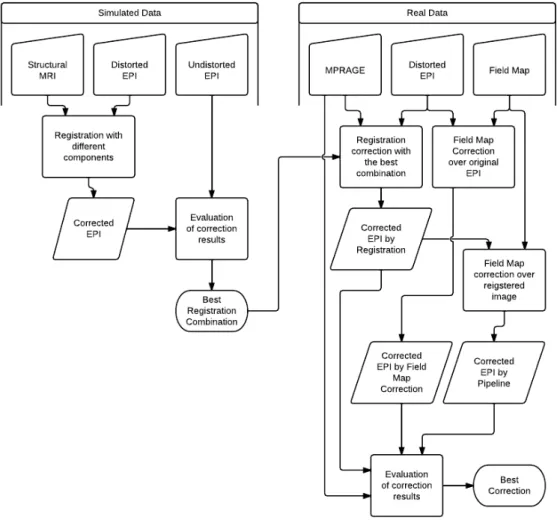
4.1 Correction process flowchart . . . 26

4.2 Simulated MRI data . . . 27

4.3 Relation between error and time of execution for the voxel size of a simulated MRI

with POSSUM . . . 27

4.5 Grid positions of reference image map compared to non-grid positions of source image . . . 30

4.6 Flowchart used to correct image using Field Map process . . . 34

5.1 Preliminary results from registration correction methods . . . 42

5.2 Distortion correction results of simulated data . . . 42

5.3 Sum of ranks of preliminary results for registration methods with simulated data . 42 5.4 Optimization ranks of Number of Bins in MI . . . 43

5.5 Optimization ranks of Number of Samples in MI . . . 44

5.6 Optimization Ranks of Learning Rate in GD Optimizer . . . 44

5.7 Optimization Ranks of Number of Iterations in GD Optimizer . . . 45

5.8 Optimization Ranks of Step Length in Powell Optimizer . . . 45

5.9 Optimization Ranks of Spline Order in B-Spline Transformation . . . 46

5.10 Comparison NMI values of pre- and post-optimization results . . . 46

5.11 Sum of ranks of post-optimization results for registration methods using simulated data . . . 47

5.12 Comparison of transformations in registration components . . . 47

5.13 Comparison of interpolators in registration components . . . 48

5.14 Comparison of optimizers in registration components . . . 49

5.15 Comparison of evaluation metrics, between real and simulated data . . . 50

5.16 Comparison between mean of ranks of simulated and real data . . . 51

5.17 Results of real data correction forb=0 . . . 52

5.18 Sum of Ranks of correction methods used in real data withb=0 . . . 52

5.19 Results of NMI for different methods andb-values . . . 53

5.20 Results of SCC for different methods andb-values . . . 54

5.21 Results of Euclidean Distance of CM for different methods andb-values . . . 54

5.22 Ranking of methods VSb-value . . . 55

7.1 Sum of ranks of registration methods in real data . . . 61

CORRECTION OF SPATIAL DISTORTION IN MAGNETIC RESONANCE IMAGING

C.1 Brain Extraction Example with BET2 . . . 82

C.2 Brain Registration Example with FLIRT . . . 84

C.3 FEAT GUI . . . 87

C.4 Procedure to a Field Map Correction . . . 88

C.5 Example of a EPI correction with Field Map . . . 89

C.6 Segmentation Example with FAST . . . 93

List of Tables

1.1 Work Plan of the project . . . 2

3.1 Registration Methods Survey . . . 22

4.1 Acquisition parameters of MRI data . . . 28

4.2 Components used in Registration . . . 38

4.3 Optimization Parameters . . . 38

5.1 Optimization Parameters . . . 43

5.2 Ranks comparison with and without RMS . . . 49

A.1 Evaluation of Preliminary Results of Registration Methods . . . 72

A.2 Evaluation of Final Results of Registration Methods . . . 73

A.3 Results of Optimization of Number of Bins in MI . . . 74

A.4 Results of Optimization of Number of Samples in MI . . . 74

A.5 Results of Optimization of Learning Rate in GD Optimizer . . . 75

A.6 Results of Optimization of Number of Iterations in GD Optimizer . . . 75

A.7 Results of Optimization of Step Length in Powell Optimizer . . . 76

A.8 Results of Optimization of Order of B-Spline in B-Spline Transform . . . 76

B.1 Evaluation of results in real data for validation of simulated data . . . 78

B.2 Results of real data forb=0 . . . 79

B.3 Mean values of NMI for differentb-values . . . 79

B.4 Mean values of SCC for differentb-values . . . 80 B.5 Mean values of Euclidean Distance CM for differentb-values . . . 80

C.1 Options of BET2 tool from FSL . . . 82

C.2 Options of FLIRT tool from FSL . . . 83

C.3 Options of PRELUDE tool from FSL . . . 84

C.4 Tissue’s Characteristics . . . 89

C.5 Options of PULSE tool from FSL . . . 90

Acronyms

ADC Aparent Diffusion Coefficient

BET Brain Extraction Tool

CLI Command-Line Interface CSF Cerebrospinal Fluid CT Computed Tomography

DOF Degrees of Freedom DTI Diffusion Tensor Imaging DW-MRI Diffusion-Weighed MRI

EPI Echo-Planar Image

FAST FMRIB’s Automated Segmentation Tool Brain Seg-mentation and Bias Field Correction

FFT Fast Fourier Tranform FID Free Induction Decay

FLIRT FMRIB’s Linear Image Registration Tool fMRI Function MRI

FMRIB Oxford Centre for Functional MRI of the Brain FNIRT FMRIB’s Nonlinear Image Registration Tool FOV Field of View

FSL FMRIB’s Software Library

FUGUE FMRIB’s Utility for Geometrically Unwarping EPI’s

GD Gradient Descent

GM Gray Matter

GPE Phase Encoding Gradient GRE Gradient Echo Sequence GRO Readout Gradient GSS Slice Selection Gradient

GUI Graphical User Interface

ITK Insigth ToolKit

MI Mutual Information

MPRAGE Magnetization Prepared Rapid Acquisition Gradient Echo

MR Magnetic Resonance

MRI Magnetic Resonance Imaging

NMI Normalized Mutual Information NMR Nuclear Magnetic Resonance

PD Proton Density

PET Positron Emission Tomography

POSSUM Physics-Oriented Simulated Scanner for Understand-ing MRI

PRELUDE Phase Region Expanding Labeller for Unwrapping Discrete Estimates

RF Radio Frequency

SCC Squared Correlation Coefficient SD Spatial Distortion

SE Spin Echo Sequence SNR Signal-to-Noise-Ratio

SPECT Single-Photon Emission Tomography STDEV Standard Deviation

TE Echo Time

TI Inversion Time TR Repetition Time

Chapter 1

Introduction

1.1

Scope

With the need and evolution of medical imaging, Magnetic Resonance (MR) appears as a tech-nique that permits a high-resolution image without using any ionizing radiation. Consequently, Magnetic Resonance Imaging (MRI) has become a major investigation and research focus among scientific and medical communities. Due to this expansion, new hardware with superior magnetic fields and faster sequences has been developed, improving spatial and time resolution. However, these improvements result in intensity and spatial distortions that reduce the MRI quality [1], especially functional (fMRI) and diffusion-weighed MRI (DW-MRI).

Correction of spatial distortion is useful to obtain a higher image quality in faster sequences, such as echo-planar images (EPI), used in fMRI and DW-MRI. Without this correction, fMRI suffers from distortions, and all images used need to be geometrically similar. Also, DW-MR images present spatial distortions that need to be corrected, because the diffusion tensor or coefficient is calculated for each voxel [2], and without this spatial correction the voxel value corresponds to an-other position. Therefore, these calculated values in DW-MRI are wrong. Anan-other advantadge of spatial distortion correction is the optimized comparison of images from other techniques, such as Computed Tomography (CT), Single-Photon Emission Tomography (SPECT) or Positron Emis-sion Tomography (PET). Finally, another use for this correction is object measurement in MRI, since, if images are not corrected, volume and area measurements will not be accurate and cannot be compared with other measurements [3].

The main causes for spatial distortions can be related to hardware or to tissue [3]. In the second case, the correction is more difficult, as it cannot be characterized for a specific system. Regardless of the cause, every geometric distortion depends on the sequence used; and faster sequences like EPI produce a greater distortion [4]. Regarding EPI, the distortion occurs mainly in the phase-encoding direction [4].

In this study we will explore three methods for spatial distortion correction. These are Registration [5, 6], Field Map Correction [7–10] and a new proposed pipeline. The first two methods were

chosen because they are the most used in literature. Registration consists in aligning a distorted image to one that has no distortion. The image with no distortion can be an MRI (anatomical, functional or diffusion) or an image from another technique, such as CT or SPECT/PET. Field Map correction is a method that consists in calculating the phase map from two gradient echo images acquired with opposite phase-encoding directions, and the calculated field map can be used to correct the distortion of the original image. The new proposed pipeline consists in performing a Field Map correction after a registration process. This process can combine the advantages of both methods and therefore, it is expected to produce better results in EPI correction.

1.2

Presentation of the Project

This project consists in state-of-the-art evaluation regarding spatial distortion correction, and im-plementation of the most significant methods that are used nowadays. A study to achieve the optimal parameters of the two most important methods in literature will be done.

The principal objective of this project is to implement these methods and optimize them to be used in real medical images, having as a secondary objective the development of a prototype software, that integrates all these methods, to be used in Siemens Healthcare Sector’s R & D Group in Portugal. Table 1.1 shows the project’s work plan.

Table 1.1:Work Plan of the project

Month Activity 1st_{W 2}nd_{W 3}tr_{W 4}th_W

December Learn magnetic resonance imaging basics_{Research data related to artefacts and correction of image} distor-tions in MRI

January Learn magnetic resonance imaging basics_{Choose the algorithms and software to correct the spatial} distor-tion

February Detailed analysis of the chosen algorithms for spatial distortion

March

Understand Siemens’ world and in particular the Healthcare Sec-tor

Familiarization with Siemens products and solutions Basic formation on anatomy and physiology Familiarization with development software Writing a software manual for FSL

April Compare and evaluate algorithms related to spatial distortion_correction

May Compare and evaluate algorithms related to spatial distortion_correction

June

Compare and evaluate algorithms related to spatial distortion correction

Optimization of algorithms for spatial distortion correction

July

Compare and evaluate algorithms related to spatial distortion correction

Propose papers for conference

Optimization of algorithms for spatial distortion correction Elaboration of a prototype software

August Optimization of algorithms for spatial distortion correction Writing thesis

1.3. CONTRIBUTION OF THE WORK

1.3

Contribution of the Work

This project will contribute to a better understanding of the several distortion correction methods in MRI and also provide a comparison between them to better understand the distortions. This study will offer the capability of choosing a method depending on theb-value in DW-MRI.

Finally, this thesis will output a prototype software where these several methods are implemented so, in the future, Siemens SA can use them in other projects and for future research in the MRI area.

1.4

Siemens SA Presentation

With 500 production centres in 50 countries and representation in 190 countries, Siemens is spread all over the world. In Portugal, Siemens S.A. encloses two factories, software research & develop-ment centres (Lisbon and Porto) and has a significant representation all over the country through its partners and company headquarters. Since 2008, the company is organized in three major sectors: Industry, Energy and Healthcare.

The Industry Sector and its solutions address Industry customers regarding production, trans-portation and building systems. This Sector is organized in five divisions: Industry Automation and Drive Technologies, Building Technologies, Industry Solutions, Mobility and OSRAM.

TheEnergy Sectoroffers products and solutions for generation, transmission and distribution of

electrical energy. This Sector is organized in six divisions: Fossil Power Generation, Renewable Energy, Oil & Gas, Energy Service, Power Transmission and Power Distribution.

TheHealthcare Sectorstands for innovative products and complete solutions, as well as service and consulting in healthcare industry. This Sector is organized in three divisions: Imaging & Therapy Systems, Clinical Products and Diagnostics.

The Imaging & Therapy Systems provides imaging systems for diagnosis and therapy, as well as for a more effective prevention, namely Magnetic Resonance Imaging Systems (MR), Computer Tomography Systems (CT), Radiography and Angiography Systems, Positron Emission Tomog-raphy Systems (PET/CT), among others. These systems are networked with high-performance healthcare IT to optimize processes.

The Clinical Products Division focuses on specific market requirements with a dedicated strategy and providing complete and specific solutions for fields such women’s health (mammography), urology and surgery, including also the ultrasound systems.

The Diagnostics Division covers business with in-vitro diagnostics, including immune diagnos-tics and molecular analysis. The Division’s solutions range from point-of-care applications to automation of large laboratories.

Thus, Siemens Healthcare Sector is the first fully integrated diagnosis company, providing a com-plete technological portfolio for the entire supply chain in healthcare.

In Portugal, Siemens SA Healthcare Sector is a market leader in the healthcare area, known for its competence and innovation skills in diagnostic and therapy systems, as well as information tech-nologies and systems’ integration. In recent years, Siemens SA Healthcare Sector has promoted the contact and cooperation with key partners in the areas of science and biomedical technol-ogy, namely Universities and Research Institutes, establishing a knowledge network and strategic partnerships and thus promoting innovation, research and development in healthcare.

Today, the Healthcare Sector’s R&D Group in Portugal is comprised by over 15 elements, work-ing in strategic areas, such as Information Systems, Computational Imagwork-ing, Automatic Medical Imaging Analysis, Modeling and Decision Support Tools and Strategic Technology Evaluation. This work has already been demonstrated by one approved patent application, two filed invention disclosures and over ten scientific publications.

Recent Milestones in Portugal

• Breast Pathology Service in Hospital de São João in Porto, Hospital da Luz in Lisbon and Clínica Dr. João Carlos Costa in Viana do Castelo - first total patient focus units, including all necessary technologies for the complete clinical process;

• Hospital da Luz in Lisbon - first hospital in Portugal with SOARIAN®_{clinical information} system, becoming one of the most modern health care installations in Europe;

• Clínica Quadrantes, in Lisbon - in-vitro diagnostics and information technology systems, which together with a PET/CT system, complemented the existing Siemens in-vivo diag-nostic systems at the clinic;

• Universidade de Coimbra - 3 Tesla Magnetic Resonance Imaging System exclusively for neuroscience research. This unit is part of the Brain Imaging Network Grid, a scientific co-operation network which integrates the Universities of Coimbra, Aveiro, Porto and Minho.

• R & D Highlights:

– Patent number DE 10 2007 053 393, System zur automatisierten Erstellung

medi-zinischer Reports;

– F. Soares, P. Andruszkiewicz, M. Freire, P. Cruz e M. Pereira, Self-Similarity Analysis

Applied to 2D Breast Cancer Imaging, HPC-Bio 07 - First International Workshop on High Performance Computing Applied to Medical Data and Bioinformatics, Riviera, France (2007);

– J. Martins, C. Granja, A. Mendes e P. Cruz, Gestão do fluxo de trabalho em

diagnós-tico por imagem: escalonamento baseado em simulação, Informática de Saúde - Boas práticas e novas perspectivas, edições Universidade Fernando Pessoa, Porto (2007);

Chapter 2

Magnetic Resonance

MRI is based on the nuclear magnetic resonance (NMR) phenomenon that was firstly described by Felix Bloch and Edward Purcell in 1946. In the beginning this technique was only used to study molecular structures and dynamics in the fields of physics and chemistry. 30 years ago, this technique was adapted by Lauterbur and Mansfield to be used for medical purposes, creating MRI [11].

2.1

Nuclear Magnetic Resonance

NMR is based on nuclear spins of Hydrogen atoms present in the human body. When a magnetic field (B0) is applied to a volume the Hydrogen atoms starts to precessing at a specific frequency, the Larmor frequency (ω0), in the orientation of theB0 field, conventionally z or longitudinal orientation. This precessing frequency is also dependent of the gyromagnetic ratio of the element (γ), as showed by equation (2.1).

ω0 =γB0 (2.1)

The sum of energy of the spins precessing is the magnetizationM, and it is the base of NMR.

To create a MR signal, magnetizationM needs to be moved from the longitudinal orientation to the transversal plane, for that, a pulse of radio frequency (RF) is used that consists in applying a magnetic field (B1) during a short period of time (1-5 ms). This pulse rotates atω0 frequency in transversal plane in phase with theM vector, which provokes resonance of the Hydrogen spins [11, 12].

With this RF pulse, theM vector produces a magnetic field that can be measured by a transversal coil, applying the Faraday’s law of induction. This signal tends to decay after the RF pulse, because the spins tend to orientate with theB0 field. The decay is called Free Induction Decay (FID) and this is the simplest experience that can be done in MR.

The FID is described by the time constantsT1 andT2. T1 describes the relaxation along the main magnetic fieldB0direction (zaxis) and is given by the equation (2.2), which is obtained by solving the Bloch equation whenMz(0) = 0.

Mz(t) =M0

1−e−

t T₁

(2.2)

where M0 is the initial magnetization. This equation can be described as an exponential curve, whereT1is the time when magnetizationMzcorresponds to 63% (figure 2.1a).

T2 describes the loss of precession synchrony among the proton spins. This decay happens after the RF pulse is turned off and it is caused by loss energy in random collisions. This transversal loss of magnetization,Mxy, can be described by equation (2.3).

Mxy(t) =Mxy(0)e−

t

T₂ (2.3)

This equation is described by the exponential curve of figure 2.1b andT2corresponds to the time when transversal magnetization is 37% of the initial magnetization.

However, when a MR signal (FID) is acquired, the decay curve is not given byT2, in fact it decays faster thanT2 (figure 2.1c). This fact can be explained by additional field inhomogeneities that contribute to a dephase of spins, and the time constant isT∗

2.

(a) (b)

(c)

2.2. MAGNETIC RESONANCE IMAGING

2.2

Magnetic Resonance Imaging

MRI is a medical image technique based on NMR of the hydrogen atoms (protons) that exist in water, which is the most abundant substance in the human body. The great advantage of MRI rela-tively to other medical images, is that this technique does not use ionizing radiation, but conserves a high resolution. This technique also gives a variety of parameters that can be measured, such as proton densities (PD), relaxation times, temperature, proton motion, chemical shifts in Larmor frequencies and tissues heterogeneities that provide a great sensibility in a large range of tissues. Finally, this technique has the advantage of being capable of delivering structural and functional images that can improve the knowledge about the human body [11, 14].

2.2.1

Image Contrast

MRI images can be weighted by various parameters to emphasize different tissues, these parame-ters areT1,T2and PD [14].

To acquire an image weighted inT1 it is necessary to have a short repetition time (TR). TR is the time between two excitation RF pulses; in other words, it is the relaxion time that protons have between two excitation pulses. If a short TR is used (TR A in figure 2.2), several tissues with differentT1 have different MRI signal amplitudes. If the tissue has a shortT1, relaxation occurs faster and the signal is strong, but if the tissue has a longT1, it does not have time to relax and the signal becomes weaker (figure 2.2). However, if a long TR (TR B in figure 2.2) is used, all the tissues have time for an almost complete relaxation and the signals of all tissues are similar and strong [14].

Figure 2.2: Relationship between TR and T1 contrast [14]

When a 90° RF pulse is applied, it surges the FID signal. However, to measure a MRI signal it is necessary to apply another RF pulse to realign the spins, this pulse is called 180° pulse. After a certain time surges a spin echo (figure 2.3a). The time between the 90° excitation pulse and the echo is called echo time (TE), and the 180º pulse occurs atT E/2. If another 180º pulse is applied afterT E/2, another echo will appear with the gap time of TE after the first echo. If a series of 180° is applied pulses we can observe a decrease in the maximum of the echoes and from this decrease,T2can be measured as the time constant of the exponential decay (figure 2.3b) [14].

T2weighting is directly related to the TE. If a short TE is used (TE A of figure 2.4), the transversal magnetization does not have time to relax. Because of that, the decay occurs only at the beginning

(a) (b)

Figure 2.3: Spin echo. Application of a single 180° RF pulse (a), multi-echo sequence (b) [13]

of the relaxation, so the different tissues with differentT2 are all present a strong signal and it is difficult to distinguish them. However, if a long TE is used (TE B of figure 2.4), relaxation occurs continuously and different tissues have different signals. If the tissue has a shortT2, the relaxation is already complete and the signal becomes weak, but if the tissue has a longT2, the relaxation will not be complete and the signal is stronger [14].

Figure 2.4: Relationship between TE and T2 contrast [14]

Finally, the PD is a weighting that indicates the quantity of protons existent in a certain tissue. To measure PD, it is necessary to adjust TR and TE to reduced theT1 andT2effects in the MRI signal. The TR from the sequence needs to be long to permit a complete longitudinal relaxation of the spins, but the TE must be short, to reduce the effect of transversal relaxation, and so the signal contrast results from the quantity of protons that exists in the tissue and not from the different tissue’s decay times [14].

2.2.2

Slice Selection and Spatial Encoding

To produce an MR image, the space must be codified, because with just the main magnet fieldB0 all protons of the body have the same frequency and it is impossible to distinguish their position. To make that codification it is necessary to apply three spatial gradient fieldsG. The fieldsBithat are applied to specific positionriare given by equation (2.4).

Bi=B0+G·ri (2.4)

These gradients used in MRI have a linear variation and they are applied in each direction (x,

2.2. MAGNETIC RESONANCE IMAGING

encoding. These threes gradients plus the RF pulses and the data sampling periods are called pulse sequence, which is used to acquire a MR image [12].

In slice selection, direction z is encoded by applying a gradient in this direction (GSS) at the same time as the RF pulse. The central frequency of the RF pulse determines the location inz

where protons are excited whenGSSis applied, because every sliceziis excited to a frequencyωi determined by the gradient [12], as shown in figure 2.5.

Figure 2.5: Slice selection process. In the presence of a gradient (GSS), the total magnetic field that a proton experiences and its resulting resonant frequency depend on its position. Tissue located at positionzi will absorb RF energy broadcast with a centre frequencyωi. Each position will have a unique resonant fre-quency. The slice thickness∆zis determined by the amplitude ofGSSand by the bandwidth of transmitted frequencies∆ω. [12]

The slice thickness is related directly to the bandwidth of the RF pulse∆ω. If the gradient is steeper, the slice will be thinner and if the gradient is shallower, the slice will be thicker [12].

Now that the slice selection in z direction is done, it is necessary to encode that slice, this is called spatial encoding and it is divided in two steps: frequency encoding and phase encoding, that encode thexandyaxis [12].

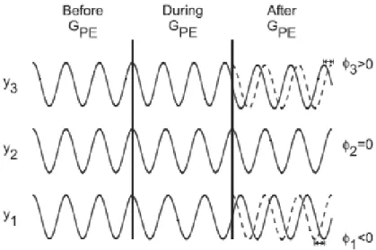
The phase encoding gradient (GP E) is normally applied along theydirection after the RF pulse and makes the protons precess at a different frequency, but when the gradient is turned off, all spins return to the original spin precessing frequency with different phase caused by the time of the gradient application, as figure 2.6 shows. So, all spins in they-axis can be identified, only by their phase [12].

Finally the frequency encoding gradient or readout gradient (GRO) is applied when the echo of the MR signal appears, making it so that only the region with a specific frequency is read [12]. The figure 2.7 shows the different frequenciesωicorresponding to different spatial positionsxi.

2.2.3

Image Reconstruction

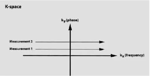
To understand the information given by the MR signal it is necessary to construct an image. The system acquires the echo with an analogue to digital converter and converts it from a time signal into a frequency signal applying a 1D Fast Fourier Transform (FFT), and this signal is stored in thek-space. k-space is a complex space that has the frequency in thekxand the phase domain in

Figure 2.6: Concept of Phase Encoding. Prior to application ofGP E, all protons precess at the same frequency. WhenGP E is applied, a proton increases or decreases its precessional frequency, depending on its position,yi. [12]

theky(figure 2.8) [15].

In most of the sequences, the signal is acquired line by line, corresponding to a different phase each line defined by GP E. In each line all the signals are acquired with different precessional frequencies generated byGRO. The number of lines and columns ink-space corresponds to the frequency samples and phase encodings performed during the MRI signal acquisition. After all

k-space is acquired an inverse 2D FFT is performed to transform phase and frequency information into contrast and spatial information [15].

2.3

Magnetic Resonance System

MR systems essentially consist in the main magnet, the magnetic field gradient system and the RF system, and can be represented by figure 2.9.

The main magnet is the principal component of the MR system and it aims to create a homoge-neous and strong magnetic field. Presently, two types of magnets are used: the permanent magnets and the super-conducting magnets. The permanent magnets have a magnetic induction between 0.01 and 0.35 T, while the super-conducting magnets can reach values of 9 T, but they are more expensive because they require permanent cooling of liquid helium [13].

The magnetic field gradient system consists in three gradient coils responsible for producing the gradient fields used for slice selection and spatial encoding. To produce the field gradients, it is necessary to produce RF that need to be switched on and off at a very fast speed that can achieve 200 to 400 T/m/s, so the coils must be very reliable and stable. However, these coils have a maximum amplitude of 20 to 40 mT/m [13].

2.4. MRI PULSE SEQUENCES

Figure 2.7: Readout Process. Following excitation, each proton within the excited volume (slice) precesses at the same frequency. During detection of the echo, a gradient (GRO) is applied, causing a variation in the frequencies for the protons generating the echo signal. The frequency of precessionωifor each proton depends upon its positionxi. [12]

Figure 2.8: k-space. kx is the frequency axis,ky the phase axis. Data from each measurement fills a different horizontal line. [14]

and is constituted by the RF antennas (coils), the RF transmission amplifier and RF receiving amplifier [13].

2.4

MRI Pulse Sequences

A pulse sequence is a series of events such as RF pulses, gradient waveforms and data acquisi-tion that produce the desired MRI signal. Different manufacturers of MRI systems use different acronyms to define a pulse sequence, and so in this thesis we will use Siemens acronyms. Gener-ally, the pulse sequences can be grouped into one of the following [16]:

• Spin echo

– Conventional Spin Echo

Figure 2.9: MRI system components [13]

– Fast Spin Echo

• Inversion recovery

• Gradient echo

• Ultra-fast imaging

To produce a spin echo (SE) sequence, it is necessary to apply a 90º excitation pulse, followed by a 180º rephasing pulse (figure 2.10). This pulse sequence is the most used for the majority of MRI applications, because it is useful to show anatomy with a high Signal-to-Noise-Ratio (SNR).

2.4. MRI PULSE SEQUENCES

In fast spin echo sequences (TSE), only a pulse of 90º is used for the acquisition of more than one readout line, and after that, a train of 180º pulses is applied to acquire several lines (figure 2.11). This technique decreases the acquisition time, but can worsen image contrast.

Figure 2.11: Fast Spin Echo Sequence [14]

The inversion recovery sequence (IR) consists in applying a 180º inversion pulse that changes the magnetization and after a time of inversion (TI), a 90º excitation pulse is applied to acquire the signal from transversal magnetization. This technique has the advantage to suppress some tissues, because if we choose the right TI, the tissue in cause can have a null longitudinal magnetization and will have no MR signal (figure 2.12).

Figure 2.12: Inversion Recovery Sequence. Following the 180° inversion pulse (a), the longitudinal magnetization vector points in the opposite direction (b). T1 relaxation takes place fromzto+z(c, d). No signal forms as long as there is no vector component in the transverse plane (the null point of a tissue) [14]

The gradient echo sequence (GRE) has the principle to use a variable flip angle(α)pulse smaller than the 90º pulse. That makes the acquisition time shorter because TR can be smaller. After applying the flip angle pulse, a gradient is used to rephase the FID instead of the 180º pulse and create the echo (figure 2.13). The TE can become shorter and thus can the acquisition time. This sequence has the disadvantage that it cannot remove the field inhomogeneities, so the signal comes always with some weighting ofT∗

2.

Recent research in MRI describes some pulse sequences that are capable of acquiring several slices in one breath hold. Usually, this technique uses GRE sequences where the excitation pulse is not totally applied, reducing the TE and so the time of acquisition. The most used ultra fast sequence is the echo-planar image (EPI) that can be done with SE and GRE. In this sequence, a slice of thek-space is acquired with a single excitation pulse just by generating multi echoes, and each phase is encoded by different slopes of gradient (figure 2.14). In a conventional SE sequence, the

k-space is acquired line by line, usually from the left to the right, and with every new excitation pulse, begins a new line. On the other hand, EPI sequence has just one excitation pulse per slice,

Figure 2.13: Gradient Echo Sequence [14]

so it is impossible to begin a new line. To resolve this problem a blip gradient is applied that inverts the field and a new line is acquired in the opposite direction. The great disadvantage of this sequence is that the resolution is lower compared with other MRI pulse sequences. However, this technique can produce very fast images that can be used in fMRI and DW-MRI.

Figure 2.14: EPI Sequence [14]

2.5

Diffusion-Weighted MRI

2.5. DIFFUSION-WEIGHTED MRI

The standard method to measure diffusion movement consists in applying a pair of symmetric gradient pulses before and after the 180º RF pulse (figure 2.15). This will increase the dephased spins in a SE, and therefore they will not rephase at TE, producing a signal loss. This method was first developed by Stejskal and Tanner [12].

Figure 2.15: Spin echo pulse sequence showing diffusion gradients, known as the Stejskal–Tanner ap-proach. Gis the amplitude for each of the gradient pulses,tis the duration of the gradient pulse during which the diffusion weighting occurs, andTis the time between the two pulses. [12]

The sensitivity to the motion in this technique is measured by field strength coefficient (b-value) that can be calculated by equation (2.5). To obtain a greater sensitivity, it is necessary to have a higherb-value. For that, several options exist, such as larger gradient amplitudes (G), longer duration of gradient pulses (t) or longer times between pulses (T).

b=γ2G2t2(T−t/3) (2.5)

The loss of signal can be described by equation (2.6).

S(T E) =e−T E/T2∗e−b∗D (2.6)

It is very difficult to measure the diffusion coefficient D, because blood perfusion also causes diffusion movements that cause a loss of signal [12]. Therefore, theapparent diffusion coefficient (ADC) is measured, which is an approximation of the D value. To measure ADC, a set of images is acquired with differentb-values and theADCvalue is extrapolated from equation (2.6), replacingDbyADC [12].

To measure the diffusion in other directions, it is only necessary to change the gradient direction. With just 6 directions, the entire geometry representable by an ellipsoid can be calculated. This technique is calleddiffusion tensor imaging(DTI), which can also be performed with more direc-tions. DTI is specially used for fibre tracking - tractography in the white matter, which consists in calculating the course of a fibre in the brain.

Chapter 3

Spatial Distortion

Artefacts in MRI are voxels that do not represent exactly the anatomy in study [12]. Some artefacts are easy to identify, but others are not, namely the artefacts that provoke a small variance in voxels. One approach to categorize artefacts is to divide them by the cause of signal misregistration [12] in three classes: Motion Artefacts, which include gross physical movement of the patient and internal physiologic motion such as cardiac and peristaltic movement and blood flow; Sequence/Protocol-Related Artefacts that are a consequence of a particular measurement technique or parameters; and External artefacts that are caused by a malfunction of the MR system or a source external to the patient and scanner. In this last one, we can include Spatial Distortions and Intensity Distortions. However, there are many other ways to classify artefacts. In this thesis only Spatial Distortions will be approached and also some methods for their corrections.

3.1

Spatial Distortion Causes

The Spatial Distortions, or according to some authors Geometric Distortions, in MRI can be classi-fied into two groups: hardware-related and tissue-related, depending on the cause of the distortion. The hardware-related distortions are caused essentially by the inhomogeneity in the main magnet, the nonlinearity in the gradient fields and the eddy currents associated to switching gradient coils.

The magnet field’s inhomogeneity is caused by deformations in the main magnet, which will produce a different magnetic excitation in the hydrogen atoms, and therefore will produce errors in the readings, because the spins are not excited in the way it was predicted. This can easily be corrected using shimming coils to adjust the inhomogeneities of the main magnet [3, 4, 12]. According to Wang and Doddrell [3] inhomogeneities distortion decreases with the increase of the used gradient strength, for instance in a MR with 1,5 T with a gradient of 1,5 mT/m, the distortion is of 1mm, but if the gradient is 3 mT/m, the distortion will be half of the anterior. This cause of distortion occurs along the readout and slice selection direction, but not along the phase encoding direction, as phase encoding is not sensitive to any field inhomogeneities.

The nonlinearity in gradient fields causes distortion and the system that reconstructs the image

expects that the gradients have no deviation and are temporally stable. This distortion appears on the periphery of the Field of View (FOV), when it is larger than 35 cm [15]. Finally, the eddy currents artefacts are due to the fast switching of the gradient coils, which causes currents in the patients, cables and wires around the patient or in the magnet itself. These currents will appear as a signal drop in the margin of the image, and the distortion is reduced by optimizing the sequence of the gradient pulses [14].

According to Holland et al. [10], "increasing the main field strength or the time to acquire a frequency-encoded line will proportionally increase the distortion". These problems are present in SE and GRE EPI, but in the second two more problems occur. This is due to the well-known through-plane dropout in regions of susceptibility change and the in-plane dephasing. The fact that spatial distortions worsne with increasing field strength is corroborated by Cusacket al[17], who explain that with the increase of the static field, the susceptibility differences become larger and so the spatial distortions also increase.

The causes for the distortions provoked by the tissues are susceptibility difference and chemical shift. It is difficult to correct the spatial distortion caused by the tissue and a dedicated correction is needed, unlike the distortions caused by hardware that can be measured and characterized for an individual system [3].

The susceptibility difference has the same effect as the main magnet field inhomogeneities, be-cause it produces a non-homogeneous magnetic field. This difference occurs in great changes of the magnetic susceptibilities. In most of the cases, this occurs in tissue-air interfaces, such as lungs or nasal cavities. Another way to produce this effect is when the tissue has some metal in its vicinity, which will also interfere with the magnetic field. The susceptibility difference will produce a quicker dephasing of spins (T∗

2) [15]. One way to prevent this distortion, when related to the presence of metal in the proximity, is to be careful with its presence every time that a MR exam is performed, due to its influence in the magnetic field

Independently of the cause of the spatial distortion, the sequence used in image acquisition influ-ences the distortion, so all the distortions are sequence-dependent and can occur in all kinds of MRI techniques such as structural, functional, diffusion, etc.[3]. Faster sequences usually cause more spatial distortion; this is the case in EPI sequences that cause a pixel shift in the phase en-coding direction [7, 10]. This is caused by the relatively long time between sampling points in that direction when compared to the frequency encoding direction [10]. This kind of sequence and spiral imaging pulse sequence cause spatial distortion due to the fast acquisition times and the magnetic field inhomogeneities [4].

3.2

Spatial Distortion and Phantoms

dimen-3.2. SPATIAL DISTORTION AND PHANTOMS

sions, but they are simple to use and the spatial distortions are easily perceptible [3]. Nowadays, already exists a significant quantity of 3D phantoms, and Wanget al.[3, 18] proposed a new 3D phantom design (shown in figure 3.1a) that consists of grid sheet layers aligned in parallel with equal spacing along the z axis. The great advantage of this phantom is that it can incorporate as many control points as the user wants, just by decreasing the gap between the grids, and it is easy to understand and measure the spatial distortion.

Other similar phantom proposed by Mattilaet al.[19] consists in a series of acrylic plates aligned in spherical holes that can be filled with the desired liquid (see figure 3.1b). This phantom was designed with dimensions that allow studying more effectively the images acquired with EPI se-quences, because the reference structures are large enough to be sampled in the EPI voxel sizes, and small enough to not have a high structure density and cause overlap of signals from different structures. The second phantom is already designed for fMRI e DW-MRI images, but it cannot measure diffusion yet.

In the field of diffusion MRI, Perrin et al.[20] developed a phantom that permits studying the white matter fibre crossing. As shown in figure 3.1c, this phantom is constituted by 2 cross sets of fibres with dimensions similar to the axons that are parallel in each set, mimicking the human white matter fibres. These fibres are permeable, which is important to allow water molecules to exchange between both extra- and intra-compartments, simulating intra and extra molecular diffusion.

(a)Wanget al.phantom[3, 18] (b)Mattilaet al.phantom[19]

(c)Perrinet al.phantom[20]

Figure 3.1: Phantoms used in MRI to measure and correct spatial distortions

3.3

Spatial Distortion Correction

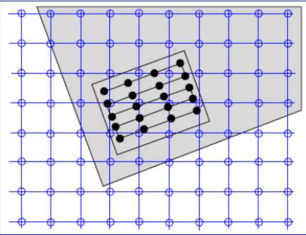
By 2005, spatial distortion correction in MRI was performed only in 2D, but it was expected that 3D methods become available soon [3]. To execute a distortion correction it is necessary to find the functions that transform the distorted image space into the undistorted space, these functions are called mapping functions [3]. These functions can be derived using 2D or 3D phantoms using the information about the distortion given by them, as explained in section 3.1

Several methods have been published to correct spatial distortions in diffusion weighted images, such as the use of gradient pre-pulse [5]; bipolar gradients [5]; twice-refocused SE [5]; calibration data [5]; acquisition of additional images with reversed diffusion gradients [5]; use RF refocusing, as in single shot spin-echo, multishot or steady state free precession pulse sequences in combina-tion with parallel imaging [1] and retrospective correccombina-tion methods [4, 5]. The advantage of the retrospective methods, such as Registration, is that they do not need a sequence modification or additional data acquisition.

Another way to correct spatial distortion is the use of shim coils [17] that also have the advantage of not needing any additional data acquisition or specific sequence, but a calibration before the image acquisition is necessary and according to the author this correction does not remove all spatial distortions in the MRI.

There are several approaches to correct MRI with a spatial distortion. In this thesis three meth-ods will be studied: Registration, Field Map correction and a new proposed pipeline. The first two methods were chosen because they are the most implemented in the referenced literature for DW-MRI correction that uses EPI sequences. The pipeline consists in performing a Field Map correction after a registration was performed, and analysing the improvements regarding the other two methods.

3.3.1

Registration

3.3. SPATIAL DISTORTION CORRECTION

can also present spatial distortion. Thus, this method requires always an image without spatial distortion or the correction will not be totally efficient.

Registration techniques can be categorized as rigid or non-rigid, depending on the type of trans-formation existent between the two images. Rigid models are usually used for rigid motion cor-rection, when it is merely necessary to determine rotation and translation [6]. However, if the deformation is non-linear, the model used must be non-rigid, because the rigid motion model will not produce an optimal alignment [6].

Registering two images consists in determining the geometric transformation that matches one image to the other. However, this problem has no easy solution. To better understand this issue, it can be divided into four components [21]:transformation model,interpolator,similarity metric and optimizer. These four components are applied to obtain transformation that approximates closely thesource image(moving image) to thereference image(fixed imaged), as shown in the diagram of 3.2. An example of an "ideal" registration is presented in figure 3.3.

Figure 3.2: The basic components of the registration framework are two input images (fixed and moving images), a transform, a metric, an interpolator and an optimizer [21]

(a)Source (b)Target (c)Registration Result Figure 3.3: Flowing from source to target: An "ideal" experiment [6]

Several studies have been developed in the field of MRI distortion correction by applying the method of Registration. Table 3.1 summarizes the set of methods studied with different registration components. It should be noted, that the Haselgroveet al.[22] study is also based on a method to register DW-MRI, where the second DW-MRI is registered to the first (b=0) and the transformation of the other DW-MRI is estimated based on theb-value.

Other studies were elaborated, but not in the field of Registration components. Mohammadiet al. [23] compares 2D and 3D registration to correct spatial distortion due to eddy-currents, concluding that a whole-brain registration will be more accurate than only a 2D registration. Daessleet al.[24]

in turn, developed a new optimization algorithm, NEWUOA (New Unconstrained Optimization Algorithm), applying it to some already existing registration methods; good results were obtained in terms of NEWUOA’s accuracy and robustness in different registration cases.

Regarding optimization of registration speed performance, some studies have been made with multi-scale Registration, such as the Maeset al.study [25]. Multi-scale resolution begins the reg-istration process with a lower resolution image (just part of the voxels are considered), converges the registration and then increases the resolution. This process is repeated to achieve the resolution of the original image. This process demonstrated to be computationally faster and the accuracy and precision of the registration continues to be good.

Table 3.1:Registration Methods Survey

Reference Metric Optimizer Interpolator Transform

Mangin[26] MI with Parzen Window_{Correlation Ratio} Powell Affine

Lau[27] MI Robbins-Munro GD B-Spline

Maes[28] MI Powell Nearest Neighbour Rigid Body

Rohde[29] NMI Gradient Ascent

Netsch[30, 31] _{Local Correlation}MI Least-Squares Affine

Wu[32] MI B-Spline Affine

Mistry[33] MI Lavenberg-Marquardt

Linear _Affine

Cubic

Fourier Fourier

Haselgrove[22] Normalized Cross Correlation Translation, Shearing and Scaling

Kim[34]

MI SPM-based Affine

Standard Deviation AIR-based Affine

AIR-based nonlinear transformation

Techavipoo[5] NMI Powell

Linear

Translation,Shearing and Scaling Partial Volume Estimated Histogram

Shift Theorem Nearest Neighbour MI = Mutual Information; GD = Gradient Descent; NMI = Normalized Mutual Information

3.3.2

Field Map Correction

According to Jezzard and Balaban [7], correcting spatial distortions in EPI with registration is difficult or impossible. The main cause of distortion in EPI is magnetic field inhomogeneities, which causea pixel shift in the phase-encoding direction and therefore, a spatial distortion. A possibel solution for this problem is to acquire a Field Map after the EPI.

A Field Map is a complex MRI that consists in acquiring two GRE images with differentT Eand subtracting the phase between them, obtaining an image that represents the field-inhomogeneity. This occurs because a phase image represents the signal given by equation (3.1) and the result of the phase subtraction is given by (3.2), where∆Φ(~r)represents the field-inhomogeneities [10].

exp(−iγ∆B(~j)T E (3.1)

3.3. SPATIAL DISTORTION CORRECTION

This way it is possible to find temporal field-inhomogeneity changes. This leads to the necessity of acquiring additionalk-space data, which increases the acquisition time and, to avoid this, the field map usually is constrained by a low-pass filter or truncated from the total EPIk-space data [35].

Another way to acquire a field map is proposed in [7, 35, 36] and consists in collecting a pair of EPI images with opposing blipped phase encode gradient polarity that contain similar spatial distortion, but in opposite directions of the phase-encode direction. This method could induce some errors as it is necessary to change the acquisition sequence and this could induce some field-map changes, especially in regions with susceptibility induced field inhomogeneity [35]. Another disadvantage of this method is that the images need to be acquired twice, which will increase the scan time.

The field inhomogeneity map can be obtained according to the expression proposed by Jezzard and Balaban [7]:

∆B(x, y, z) = ∆Φ(x, y, z) 2πγ∆TE

(3.3)

where∆Φrepresents the difference phase map of the two structural images,γ is the gyrometric ratio for hydrogen and∆T E is the difference between echo times. The authors also established that a smooth operation before the phase map calculation is beneficial, so as to prevent abrupt transitions between distinct images regions. Whit this method it is possible to correct spatial distortion in the phase-encoding directions.

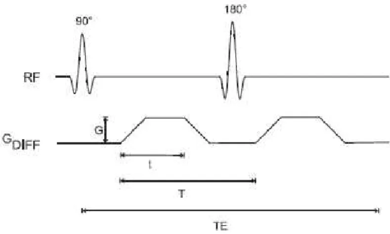
Gallichanet al. [36] propose a sequence that can be useful to acquire the Field Map onin vivo MRI exams. This sequence (see figure 3.4) consists of an additional spin-echo with reversed phase-encoding direction instead of the standard spin-echo used in DTI, which has the advantage of minimizing the scan time, comparatively with a double acquisition. This sequence can be improved with the use of parallel acceleration that reduces the TE and increases the SNR.

Figure 3.4: Proposed pulse-sequence diagram for dual-echo blip-reversed diffusion-weighted EPI [36]

Chapter 4

Methodology

As established in previous chapters, spatial distortion is an MRI issue that must be corrected for better visualization medical images. This project proposes study and comparison of several methods to correct this distortion: Registration, Field Map correction and a new proposed pipeline, which consists in performing a Field Map correction after a registration process. As a result, we expect to obtain comparisons between the three proposed methods for DW-MRI data with different field strength coefficients (b-values) and to assess how this coefficient influences accuracy and performance of these methods. As a conclusion of this project, we expect to establish the best correction method for DW-MRI for a givenb-value.

Registration and Field Map correction are methods already described in literature. However, the combination of methods has not been studied yet. This pipeline combines advantages of two correction methods: Registration alignment and resampling, and specific correction of field in-homogeneities for Field Map correction. Another reason for choosing these methods was the implementation simplicity, when compared with other methods in literature. An advantage of these methods is that they are already totally or partially implemented. In the case of the Registra-tion, the ITK[37] library inC++has an extensive set of components and FSL [38, 39] has some registration components implemented, as well. FSL has the Field Map correction method already implemented, which will simplify the implementation part of the project.

For assessment of registration correction results, simulation of MRI data was required, in order to obtain images with distortion and their corresponding images without distortion. Simulated data was used to optimize registration parameters, in order to achieve optimal parameters for all combinations tested.

Registration combinations with new optimized parameters were tested and evaluated, by applying the metrics described in this chapter. Also, the same combinations of Registration were performed and evaluated forb=0 real data, to validate the simulated data correction. The best combinations were then used with real data. For that purpose, real DW-MRI data is acquired with differentb -values and used to assess the three methods proposed, namely: Registration, Field Map correction and the new proposed pipeline and the correction accuracy in images with increasingb-values that

correspond to a decrease in SNR. We chose this type of image due to its great need for correction and the existing general need for a comparative study of these methods using this type of images, as it is poorly represented in reviewed literature.

The flowchart in figure 4.1 explains the procedure that was applied in this project.

Figure 4.1:Correction process flowchart

4.1

Simulated Data

This part of the project ensures the evaluation of registration correction accuracy, as it is possible to simulate EPI data with and without distortion and structural images.

4.2. DATA ACQUISITION

Also, a structural image was necessary to perform registration. For that, POSSUM [40, 41] was used again to generate a GRE with T E = 35.7ms, T RSlice = 150ms, T R = 685,44s, a resolution of 3x3x3 mm3_{and a size of 64x64x50 (figure 4.2c).}

(a)Distorted EPI (b)Non-distorted EPI(c)Gradient-Eco MRI Figure 4.2:Simulated MRI data

Regarding simulated data, it is important to say that they could have associated errors; this means that they do not completely represent the real data. In the case of POSSUM, Drobnjak and Jenk-inson studied the influence of the voxel size in the error of the image [40], as shown in figure 4.3, where it is demonstrated that with increasing voxel size, the associated error also increase. With the voxel size used in this project (3x3x3 mm3) the associated error between analytical and simu-lated data is of3%. It is also important to state that this analysis is not a comparison between real and simulated data. However, it is closer, so it is important to validate simulated data. Another analysis performed by Drobnjak and Jenkinsonet al. [40] was the time of simulation, related to the voxel size. However, this analysis was performed for normal simulations and this project used simulation with aB0field that increases the simulation time.

Figure 4.3: Relation between error and time of execution for the voxel size of a simulated MRI with POSSUM. The black line and blacky-axis show the RMS based difference between the analytically

cal-culatedk-space and simulatedk-spaces expressed as a percentage of the analytically calculated k-space signal. The red line and the redy-axis show the computational time which it took for the generation of the simulations [40]

4.2

Data Acquisition

Real data was obtained with a 3T Siemens MAGNETOM TRIO Tim system at IBILI. A distorted set of DW-MRI withb-values of 0, 1000, 4000 and 8000 was obtained. Acquisition parameters are described in table 4.1.

We acquired a structural MPRAGE image to correct the EPI distorted by Registration methods and a gradient echo field map image to correct with the Field Map method. This field map image was acquired with a∆T E of7.38ms. Acquisition parameters of both images are also presented in table 4.1.

Table 4.1:Acquisition parameters of MRI data

b-value TR(ms) TE(ms) FA(◦) TI(ms) FOV(mm3_{) Resol.(}

mm3_{) Matrix Size} EPI

0 11300 121

90 - 256x256x120 2x2x2 128x128x60 1000 11300 121

4000 12600 142 8000 14700 178

MPRAGE - 2980 2300 9 900 256x256x160 1x1x1 256x256x256

Field Map - 423 - 60 - 256x256x120 4x4x3 64x64x40

(a)MPRAGE (b)EPI -b=0 (c)Field Map Figure 4.4:Real MRI data

4.3

Registration

As already explained in section 3.3.1, Registration consists in finding the best transformation that matches the source image to the reference image. This can be translated by equation (4.1) where

Ais the reference image,Bthe source image transformed byT(),M()the similarity metric and

arg()represents the transformation argument ofT [42].

argmaxM(A, T(B)) (4.1)

In this section, several components (transformations, interpolators, metrics and optimizers) used in various registration techniques will be explained. All the components used are already imple-mented in ITK [37], and the following explanation is based on software features that are explicit in the ITK guide [21].

4.3.1

Transformations