Influence geometric anisotropy in management zones delineation
1Influência da anisotropia geométrica na delimitação de zonas de manejo
Danilo Pereira Barbosa2*, Eduardo Leonel Bottega3, Domingos Sárvio Magalhães Valente4, Nerilson TerraSantos4, Wellington Donizete Guimarães5 and Matheus de Paula Ferreira4
ABSTRACT - The proper handling soil allows the reduction of contaminants, maximize agricultural productivity, and is directly related the knowledge spatial variability of soil attributes. This spatial variability can express isotropic and anisotropic form. The latter being neglected in research related to management zones delineation. In this context, the present study aimed to evaluate the effect of the geometric anisotropy correction on the management zone delineation. The methodology was applied under database of soybean productivity and apparent electrical conductivity (CEa) of a rural property in Ponta Porã – MS. By means of this georeferenced database, maps was interpolated with ordinary kriging. For each combination, attribute (productivity and CEa) and number of classes, were produced two maps management zones, one without and one with anisotropy correction, the same were compared through the kappa index, with significance tested by the Z-test. The management zones number was also evaluated by Fuzziness Performance Index (FPI) and the Modified Partition Entropy (MPE). The area subdivision in two management zones, without and with anisotropy correction, presented higher Kappa index, with values of 0.89 and 0.91 respectively, but not presented significant differences with each other.
Key words: Geostatistics. Anisotropy factor. Spatial variability. Apparent electrical conductivity. Soybean.
RESUMO - O manuseio adequado do solo, além de permitir a redução de contaminantes e a maximização da produtividade agrícola, está diretamente relacionado ao conhecimento da variabilidade espacial dos atributos do solo. Esta variabilidade espacial pode expressar-se de forma isotrópica e anisotrópica. Sendo a última, negligenciada nas pesquisas relacionadas ao delineamento de zonas de manejo. Nesse contexto, o presente trabalho objetivou avaliar o efeito da correção da anisotropia geométrica na delimitação de zonas de manejo. A metodologia foi aplicada sob um banco de dados de produtividade de soja e condutividade elétrica aparente (CEa) de uma propriedade rural em Ponta Porã - MS. Por meio deste banco de dados georreferenciados interpolou-se mapas com uso da krigagem ordinária. Para cada combinação, atributo (produtividade e CEa) e número de classes, foram produzidos dois mapas de zonas de manejo, um sem e outro com a correção da anisotropia, onde os mesmos foram comparados por meio do índice kappa, com significância testada pelo teste Z. O número de zonas de manejo foi avaliado quanto ao Índice de Performance Fuzzy (FPI) e a Entropia da Partição Modificada (MPE). A subdivisão da área em duas zonas de manejo, sem e com correção de anisotropia, apresentou maior índice kappa, com valores de 0,89 e 0,91 respectivamente, não apresentando diferenças significativas entre si.
Palavras-chave: Geoestatística. Fator de anisotropia. Variabilidade espacial. Condutividade elétrica aparente. Soja.
DOI: 10.5935/1806-6690.20190064 * Author for correspondence
Received for publication 15/05/2017; approved on 29/03/2019
1Parte da Tese do primeiro autor, apresentada ao Programade Pós-Graduação em Estatística Aplicada e Biometria, Universidade Federal de Viçosa/ UFV
2Departamento de Estatística Aplicada e Biometria,Universidade Federal de Viçosa/UFV, Viçosa-MG, Brasil, [email protected] (ORCID ID 0000-0001-5117-4009)
3Universidade Federal de Santa Maria/UFSM, Cachoeira do Sul-RS, Brasil, [email protected] (ORCID ID 0000-0003-4035-6880)
4Universidade Federal de Viçosa/UFV, Viçosa-MG, Brasil, [email protected] (ORCID ID 0000-0001-7248-8613), [email protected] (ORCID ID 0000-0003-0334-6640), [email protected] (ORCID ID 0000-0002-4110-9147)
5Instituto Federal de Educação, Ciência e Tecnologia Goiano, Rio Verde-GO, Brasil, [email protected] (ORCID ID 0000-0002-8642-8141)
INTRODUCTION
The soybean culture presented, in the 2017/18 harvest, an estimated production of 336.7 million tons, in an area planted estimated at 90.1 million hectares (UNITED STATES DEPARTMENT OF AGRICULTURE, 2018). However, this formidable scenario does not present homogeneous productivity, being observed variations in small areas of cultivation (BOTTEGA et al., 2017a), that may be associated to the spatial variability of the nutrients present in the soil (FAGUNDES et al., 2018; RICARDO et al., 2016) and to the effects of complex interaction between soil chemical properties and culture management practices (BOTTEGA et al., 2013; PEREIRA et al., 2016).
Geostatistics allows identifying these areas with low productivity as well as identifying factors that influence it. Knowledge of the spatial variability pattern of these factors allows treatment at variable rates in the subregions of the field. These subregions are referred to as management zones. The management zone can be defined as a subregion of the field that needs to receive the input dosage uniformly, as it presents the same levels of factors limiting crop productivity (RODRIGUES JUNIOR et al., 2011). Its use allows soil conservation (DALCHIAVON et al., 2012), reduction of production costs and environmental impacts (BOTTEGA et al., 2017b).
Among the issues surrounding the generation of management zones, it is essential to identify the main parameters in its implementation (FRIDGEN et al., 2004). In this sense, we highlight the use of the apparent electrical conductivity (CEa) of the soil, whose pattern of spatial variability relates to the pattern of spatial variation of cultures and soil physical and chemical properties (CORWIN et al., 2003). Morari, Castrignano and Pagliarin (2009) used CEa values and other soil physical properties to characterize spatial variability using kriging. The results of this study allowed isolating sources of variations that acted at different spatial scales. These sources of variation made it possible to delimit management zones through the fuzzy k-means algorithm. Molin and Castro (2008) and Bottega et al. (2017b) also used CEa data and soil properties in the characterization of spatial variability by means of ordinary kriging. The interpolated maps were used in the delimitation of management zones applying the fuzzy K-means method.
In view of the mentioned studies, it is well known that the variability of soil attributes, especially CEa, can help to delimit management zones when using classification methods. The spatial variability of these attributes has been modeled and mapped by means of geostatistical linear predictors. The use of these maps
makes it possible to explain the causes of production variability (QUEIROZ et al., 2000).
In the delimitation of management zones the maps of variability have been generated using several geostatistical interpolators such as ordinary kriging (ALVES et al., 2013; CHANG et al., 2014; FU; WANG; JIANG, 2010; MORAL; TERRÓN; REBOLLO, 2011; SAFANELLI; BOESING; BOTTEGA, 2015; TRIPATHI et al., 2015), the co-kriging (MORARI; CASTRIGNANO; PAGLIARIN, 2009), the regression kriging (MORAL; TERRÓN; SILVA, 2010), the linear programming (CID-GARCIA et al., 2013) among others.
However, these surveys have ignored the geometric anisotropy correction. Geometric anisotropy is caused when the semivariogram presents different patterns of spatial dependence in different directions. The geometric anisotropy correction allows greater precision in the construction of thematic maps that describe the spatial variability of the soil attributes (GUEDES et al., 2013). In this context, given the importance of the geometric anisotropy correction, the present work aims to evaluate its effect on the delimitation of management zones.
MATERIAL AND METHODS
The methodologies in this work were applied in a database collected by Bottega (2014) in a rural property in the city of Ponta Porã - state of Mato Grosso do Sul (MS). The soil is classified as a Dystroferric Red Latosol, with a clayey texture (EMPRESA BRASILEIRA DE PESQUISA AGROPECUÁRIA, 2013). This database contains measurements, in 160 georeferenced points, of the CEa attributes and soybean productivity in the 2011 / 2012 harvest. CEa measurements were obtained with a depth of 0 to 20 cm.
The georeferencing of the attributes was performed by a Garmin GPS receiver, model GPSMAP 62. The productivity values were obtained and manually georeferenced at sample points composed of three lines of one linear meter, with an area of 1.35 m2 being the values
expressed in kg ha-1.
For each of the measured attributes a spatial dependence model was adjusted with and without anisotropy correction. This model was adjusted to the empirical semivariogram which was obtained from the calculation of the semivariance γ(h):
(1) for different separation distances (MANTO, 2005). Where h is the distance between pairs of observations
and N(h) is the number of observation pairs Z(xi) and Z(xi+h) observed at positions xi and xi and that are separated by a distance h.
For the modeling of the structure disregarding the anisotropy correction, the weighted least squares (WLS) adjustments were applied to the Gaussian, exponential and spherical models.
The adjusted models received as initial estimates the parameters found by Bottega (2014). Each adjustment was submitted to the linear geostatistical predictor of ordinary kriging, disregarding the trend effect.
And as a selection criterion, the model that presented the lowest mean of the kriging cross-validation errors (Mean Error: ME) was used:
(2) where Ẑ(xi) is the value of the estimate at the point not
observed xi.
According to Oliver and Webster (2014), even with a poor choice of the model, the mean of errors equal to zero ensures that kriging is not biased. In addition to the ME, to guarantee the correct choice of the model, we followed the suggestion of the same author and used the Mean Squared Deviation Ratio (MSDR) with the expected ideal value, the closest to 1.
(3)
where Ẑ(xi) the kriging estimate of the variable sampled at
point xi and ô2
k(xi) the estimate of the kriging variance of
the variable sampled xi.
The selected model was then used to measure the spatial dependency index (SDI) proposed by Zimback (2001). Such index is defined as the percentage of the contribution in relation to the level. Thus, spatial dependence can be classified as: strong for IDE > 75%, moderate for IDE between 25% and 75% and weak for IDE < 25%.
All steps mentioned above were also used in the modeling whose anisotropy correction was considered. In this case, the value of the semivariogram depends not only on the length of the vector h, but also on its direction.
For each adjustment referenced above, it was followed if the steps described in Manto (2005) first identified whether the anisotropy axes (major and minor axes) by means of experimental semivariograms in different directions (0º, 45º, 90º and 135 ºc with a tolerance of 22.5º).
Then, a translation of the axes of the data matrix was made, coinciding with the axes of the anisotropy by means of the rotation matrix R:
(4) where α is the angle in the north direction with the largest axis of the ellipse. Then, the directional semivariograms are combined into a single semivariogram, where the range is normalized to size 1 using the matrix T:
(5) where αmax and αmin are the axes of the ellipse of anisotropy with greater and smaller range, respectively. Then, the rotational matrices R and translation of T axes are combined to obtain a single isotropic semivariogram, given by y(xi-xj) = y(||TR(xi-xj)||). Diggle and Ribeiro
Junior (2007) also used the same process using linear transformation (rotation and translation) through matrix A: (6) In this way, the geometric anisotropy correction is defined by the parameters α (direction of greater spatial continuity) and anisotropy factor Fα=α2/α1, being α2 and
α1, respectively, the higher and lower range values of the directional semivariograms.
All the methodological mechanisms used in the spatial dependence structure modeling were conducted with the use of Software R (R CORE TEAM, 2016) using the geoR package (RIBEIRO JUNIOR; DIGGLE, 2016).
After the spatial dependence modeling, the interpolated maps for the CEa attributes and soybean productivity were processed by the KrigMe software (VALENTE et al., 2012), which uses the fuzzy
k-means classification method to delimit the management
zones.
The fuzzy k-means classification algorithm
determines the number of management zones by means of the Fuzziness Performance Index (FPI) and the Modified Partition Entropy (MPE), that relate the disorganization of the data regarding the definition of management zones. When these two indexes have minimum values, we have the optimal number of classes established (SONG et al., 2009).
For each combination, attribute and number of classes, two maps of management zones were produced, one without and the other with anisotropy correction, where they were compared using the kappa index. This index was evaluated for its significance by the Z test, which consequently allows us to gauge the similarity
between the maps. Thus, maps whose kappa coefficient is equal to zero, are totally different. And the closer to one, the greater the similarity. Thus, limits of similarity between the maps were established by means of the kappa coefficient as proposed by Landis and Koch (1977), so that the level of similarity between maps is classified as poor for kappa values between 0.00 and 0.19, reasonable for kappa values between 0.20 to 0.39, good for values between 0.40 and 0.59, very good for values between 0.60 and 0.79 and excellent for kappa values greater than or equal to 0.80.
RESULTS AND DISCUSSION
Descriptive analysis: the descriptive statistics
associated to the productivity and CEa attributes are presented in Table 1.
Despite the difference of scale in the measurement of the attributes, the productivity presented a lower percentage variation of the data around the mean, than that presented for the CEa. Similar coefficient of variation (35.1) for this same attribute was also verified by Aggelopooulou et al. (2013). This author also obtained a distribution of CEa values with positive asymmetry). Productivity, on the other hand, presented a distribution with negative asymmetry.
Variographic analysis without anisotropy correction: where the parameters of the omnidirectional
semivariogram models selected based on the cross-validation statistics for the productivity and CEa attributes are presented (Table 2).
Table 1 - Descriptive statistics associated with productivity and apparent electrical conductivity attributes
Prod - Productivity (kg ha-1); CEa - Apparent electrical conductivity of the soil (mS m-1); N - Number of observations; SD - standard deviation; CV - Coefficient of variation (%); CA - Coefficient of Asymmetry; CK - Coefficient of kurtosis
Table 2 - Specifications of omnidirectional models adjusted without anisotropy correction
Prod - Productivity (kg ha-1); CEa - Apparent electrical conductivity of the soil (mS m-1); ME - Mean of errors of the kriging cross-validation; MSDR - Mean Squared Deviation Ratio of cross-validation of kriging, R2Adj - Adjusted coefficient of determination
Attributes N Minimum Medium Mean SV CV CA CK Maximum
Prod 160 1225,06 2.345,26 2.302,75 298,44 12,96 -0,35 0,85 3.244,49
CEa 160 2,74 5,94 6,19 2,13 34,44 2,24 9,29 19,31
Attributes Parameters
Nugget Effect Level Practical Range ME MSDR R2Adj
Prod 18.948,7 108.527 374,92 0,48 1,3 0,61
CEa 3,11 3,88 836,24 0,00 1,0 0,20
For both attributes the Gaussian model adjusted by the weighted least squares method was selected. The criterion of selection of this model resulted from the use of the mean of the kriging cross-validation errors. The lower the mean of the kriging cross-validation errors, the greater the accuracy (SILVA JUNIOR et al., 2012). Additionally, we verified the weighted mean square error of the kriging c0ross-validation, whose value should be the closest one.
The semivariogram models selected for the productivity and CEa attributes respectively explained that 83% and 20% of the total data variation are due to spatial dependence, according to the spatial dependence index by Zimback (2001).
Variographic analysis with anisotropy correction: The acquisition of directional empirical
semivariograms verified the existence of anisotropy. It was verified for the productivity attribute, anisotropy angle at 0º and anisotropy factor 1.5; while in the CEa attribute, anisotropy angle was found at 90º and anisotropy factor 2.0.
The anisotropy parameters of each attribute were applied to the linear transformations of spatial coordinates of their respective georeferenced samples. After the linear transformations in the spatial coordinates, new directional semivariograms were constructed in the directions of greater and smaller spatial continuity and respective anisotropy factor.
The parameters of the directional semivariograms of the Gaussian model obtained after transformations of the spatial coordinates are presented in Table 3.
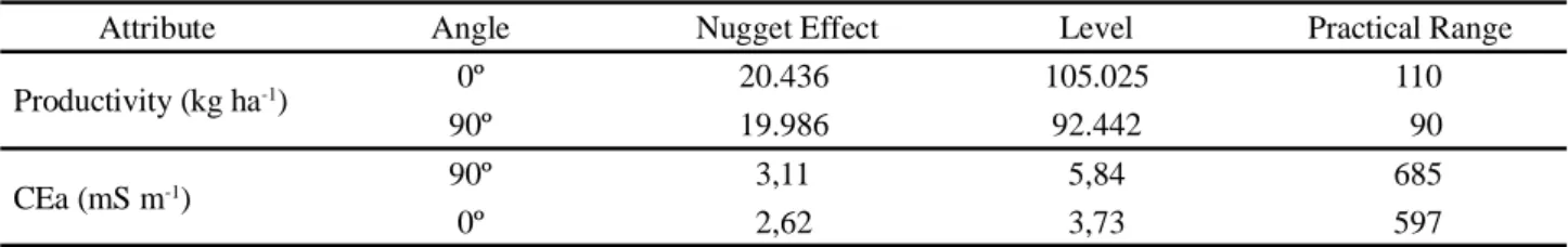
Table 3 - Gaussian model parameters of the directional semivariograms relative to the angles of greater and lesser spatial continuity, after linear transformations in the georeferenced coordinates of the attributes
Attribute Angle Nugget Effect Level Practical Range
Productivity (kg ha-1) 0º 20.436 105.025 110
90º 19.986 92.442 90
CEa (mS m-1) 90º 3,11 5,84 685
0º 2,62 3,73 597
When comparing the estimates of the semivariograms parameters adjusted at the 0º and 90º angles for the productivity attribute, a similar value is observed for the estimate of the nugget effect parameter and that the axis of greater spatial continuity is close to 20% of the axis of lesser spatial continuity. In addition, the estimate of the Level does not exceed 15% of the axis of greater spatial dependence.
Similar behavior was also observed for the CEa attribute, in which the percentage increase in the estimate of the Nugget Effect does not exceed 20%, when the estimates of the axis of lesser spatial continuity to the one of greater spatial continuity are countered. In the Practical Range estimates, only a percentage increase of less than 0.15% is observed.
These results indicate that the linear transformations were able to correct the anisotropy effect to such an extent that, when adjusting variogram on the two anisotropy axes (0º and 90º), the adjusted models presented similar estimates for the parameters (Nugget, Level and Range).
Therefore, to correct the geometric anisotropy, the georeferenced coordinates of the sampled points were submitted to linear transformations and an omnidirectional semivariogram model was obtained for each of the attributes (Table 4).
For the CEa attribute, the adjusted coefficient of determination was identical to that found in variography that disregarded the anisotropy, as well as the mean of the cross validation errors. Already the productivity attribute remained with the same adjusted coefficient of determination.
Table 4 - Gaussian model parameters of the omnidirectional semivariograms after linear transformations in the georeferenced coordinates of the sampled points where the productivity and CEa attributes were measured
Prod - Productivity (kg ha-1); CEa - Apparent electrical conductivity (mS m-1); ME - Mean of errors of the kriging cross-validation; MSDR - Mean Squared Deviation Ratio of cross-validation of kriging; R2Adj - Adjusted coefficient of determination
Attribute ME MSDR R2Adj Nugget Effect Level Practical Range
Prod 0,09 0,80 0,61 20.000 92.250 138
CEa 0,00 1,1 0,20 2,97 3,34 635
The parameters of these omnidirectional semivariogram models were then used in the linear geostatistical predictor of ordinary kriging. The use of this predictor allowed to express the spatial variability maps of the attributes.
Definition of management zones: both the maps
developed in the analysis without anisotropy correction and those developed in the analysis with anisotropy correction were submitted to the fuzzy k-means algorithm for the design of the management zones with different numbers of classes.
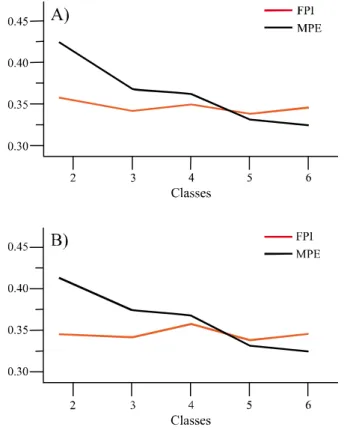
In each map produced, the Fuzziness Performance Index (FPI) and Modified Partition Entropy (MPE) were evaluated for both attributes, productivity and CEa (Figure 1).
As well as Peralta et al. (2015) and Chang et al. (2014), the indexes were evaluated in up to six classes. As can be seen in (Figure 2), for the productivity attribute, as the number of classes increases, both the indexes with and without anisotropy correction approximate zero. Already the CEa attribute presented opposite behavior.
When comparing the indexes with and without anisotropy correction, values closer to zero were obtained after anisotropy correction. These values indicate a better organization of the data in relation to the other analysis, since the FPI estimates the degree of separation of the members in different zones and the MPE estimates the degree of disorganization created by the number of zones. These indexes present values between 0 and 1, the optimal number of management zones is obtained when both indexes are minimized (SONG et al., 2009).
For each number of classes verified for the indexes mentioned (FPI, MPE), maps with their respective management zones were produced. The maps produced without anisotropy correction were compared to those corrected for anisotropy, for both attributes (productivity and CEa) for each number of classes. The comparison was made with kappa index and respective Z Test (p-value < 0.01).
Figure 2 - Kappa index, as a function of the number of classes, comparing maps with and without anisotropy correction, for productivity (Prod) and apparent electrical conductivity (CEa)
A Figure 2 shows that, as the number of classes increases, the kappa values tend to reduce, however, regardless of the number of classes, all kappa values were significant at 5% probability by the Z Test. Thus, the level of similarity between the maps compared in the productivity attribute presented an excellent classification when using two or three classes, as proposed by Landis and Koch (1977), however, for four or five classes was classified as very good.
For the CEa attribute, only with the use of two classes, the level of similarity between the maps can be classified as excellent, whereas with three classes there was a very good classification and with four or five classes, it was classified as good.
The kappa values presented in Figure 2 are similar to those obtained by Guedes et al. (2013) when comparing kriging maps with isotropic and anisotropic structure for simulated soil chemical attributes data. The same author, when considering actual values of a case study, obtained values of kappa between 0.7 and 1 for a sample of 100 observations with anisotropy factor of 1 to 5.
Thus, considering the lower values of FPI and MPE, and the significance of the kappa, it is recommended
Figure 1 - Fuzziness Performance Index (FPI) and Entropy of Modified Partition (MPE) relative to the number of classes in the delimitation of management zones for the attributes: A) Productivity, disregarding anisotropy correction; B) Productivity, considering anisotropy correction; C) CEa, disregarding anisotropy correction and D) CEa, considering anisotropy correction
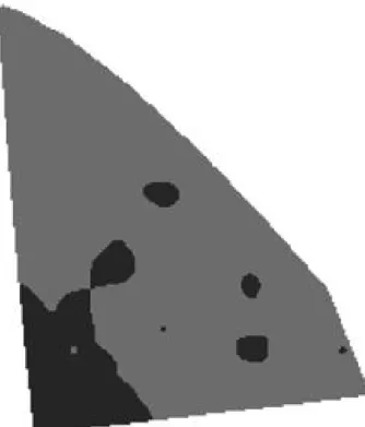
Figure 3 - Map of management zones for the CEa attribute obtained without geometric anisotropy correction
to use two classes in the generation of management zones without the need for geometric anisotropy correction. Thus, Figure 3 shows the map of management zones obtained without the anisotropy correction, for the CEa attribute aiming at obtaining higher productivity in the soybean plantation for the study area.
The area whose data were collected for this research was presented with free flow, without occurrence of ditches and/or furrows, with soil classified as Dystroferric Red Latosol, with a clayey texture (EMPRESA BRASILEIRA DE PESQUISA AGROPECUÁRIA, 2013) and excellent drainage. In cases where the soil is anisotropic or has unsatisfactory drainage, it has been modeled considering such an anisotropic characteristic (VALIPOUR, 2012; VIERO; VALIPOUR, 2017).
In addition to the occurrence of anisotropic soils, its physicochemical properties same may present anisotropic spatial dependence pattern. However, several studies have neglected this possibility (ALVES et al., 2013; CHANG et al., 2014; CID-GARCIA et al., 2013; FU; WANG; JIANG, 2010; MORAL;TERRÓN; REBOLLO, 2011; MORAL; TERRÓN; SILVA, 2010; MORARI; CASTRIGNANO; PAGLIARIN, 2009; SAFANELLI; BOESING; BOTTEGA, 2015; TRIPATHI et al., 2015).
In view of this omission, the objective was to evaluate the effect of geometric anisotropy on the delimitation of management zones for CEa data of the soil. The use of such an attribute is strongly related to the spatial variability of soybean productivity and sample questions.
The spatial variability pattern of CEa presented with Gaussian structure in both analyses, with and without geometric anisotropy correction. Such behavior is characterized by low distance variations, since it is presented continuously (ISAAKS; SRIVASTAVA, 1989). Similar results were also obtained by Bottega (2014) in disregarding the geometric anisotropy correction.
The definition of the number of management zones when using the maps obtained in fuzzy k-means was based on the FPI and MPE indexes. These indexes are based on the better separation and organization of the data in the delimitation of the management zones (RICARDO et al., 2016).
The indexes obtained were close to those found by Bottega (2014) for productivity (FPI = 0.3276 and MPE = 0.3215) and CEa (FPI = 0.2071 and MPE = 0.2668). In addition to the similarity obtained by Bottega (2014), Valente et al. (2012) also found similar values of FPI and MPE for CEa (0.22 and 0.27). Peralta et al. (2015), found lower values of FPI and MPE for CEa (0.03 to 0.07), however the depths used by the authors were 0 to 30cm and 0 to 90 cm. The authors Morari, Castrignano and Pagliarin (2009) using maps interpolated with kriging found similar values of FPI and MPE to those obtained by Peralta et al. (2015), varying between 0.06 and 0.04, however, the evaluated attributes were sand, clay and gravel.
The values obtained for the FPI and MPE indexes were lower for the corrected anisotropy maps than for the uncorrected ones ().-C and ).-D). However, the kappa index showed no significant difference in the maps of management zones with and without anisotropy correction. Thus, as much as the anisotropy correction increases the precision in the construction of thematic maps (BOISVERT; MANCHUK; DEUTSCH, 2009; CHORTI; HRISTOPULOS, 2008; FACAS; MOONEY; FURRER, 2010; GUEDES et al., 2013; ZIMMERMAN, 1993), the design of the management zones was not affected.
Similar results were found by Guedes et al. (2013) when comparing these spatial dependence structures using the kappa index. This author observed that, even with high values of anisotropy (3.4 and 4.5), there is similarity between the maps generated. This same similarity was also observed through global accuracy and Tau index.
CONCLUSION
Although the FPI and NCE indexes presented values closer to the ideal with the anisotropy correction, the kappa index did not detect a significant difference in relation to those that were obtained without the correction. Thus, it can be understood that ignoring or transforming a geometric anisotropic variable into isotropic does not necessarily significantly affect the grouping of data into classes by means of the fuzzy k-means algorithm, which in turn delimits the management zones.
REFERENCES
AGGELOPOOULOU, K. et al. Delineation of management zones in an apple orchard in Greece using a multivariate approach. Computers and Electronics in Agriculture, v. 90, p. 119-130, 2013.
ALVES, S. M. F. et al. Definição de zonas de manejo a partir de mapas de condutividade elétrica e matéria orgânica. Bioscience Journal, v. 29, n. 1, p. 104-114, 2013.
BOISVERT, J. B.; MANCHUK, J. G.; DEUTSCH C. V. Kriging in the presence of locally varying anisotropy using non-euclidian distances. Mathematical Geosciences, v. 41, n. 5, p. 585-601, 2009.
BOTTEGA, E. L. et al. Precision agriculture applied to soybean: Part III: Spatial and temporal variability of productivity. Australian Journal of Crop Science, v. 11, n. 7, p. 799-805, 2017a.
BOTTEGA, E. L. et al. Precision agriculture applied to soybean: Part I: Delineation of management zones. Australian Journal of Crop Science, v. 11, n. 5, p. 573-579, 2017b. BOTTEGA, E. L. et al. Variabilidade espacial de atributos do solo em sistema de semeadura direta com rotação de culturas no cerrado brasileiro. Revista Ciência Agronômica, v. 44, n. 1, p. 1-9, 2013.
BOTTEGA, E. L. Utilização de zonas de manejo para a produção de soja no cerrado brasileiro. 2014. Tese (Doutorado em Engenharia Agrícola) - Universidade Federal de Viçosa, Viçosa, MG, 2014.
CHANG, D. et al. Delineation of management zones using an active canopy sensor for a tobacco field. Computers and Electronics in Agriculture, v. 109, p. 172-178, 2014.
CHORTI, A.; HRISTOPULOS, D. T. Nonparametric identification of anisotropic (elliptic) correlations in spatially distributed data sets. IEEE Transactions on Signal Processing, v. 56, n. 10, p. 4738-4750, 2008.
CID-GARCIA, N. M. et al. Rectangular shape management zone delineation using integer linear programming. Computers and Electronics in Agriculture, v. 93, p. 1-9, Apr. 2013.
CORWIN, D. L. et al. Identifying soil properties that influence cotton yield using soil sampling directed by apparent soil
electrical conductivity. Agronomy Journal, v. 95, n. 2, p. 352-364, 2003.
DALCHIAVON, F. C. Variabilidade espacial de atributos da fertilidade de um Latossolo Vermelho Distroférrico sob Sistema Plantio Direto. Revista Ciência Agronômica, v. 43, n. 3, p. 453-461, 2012.
DIGGLE, P. J.; RIBEIRO JUNIOR, P. J. Model-based Geostatistics. New York: Springer, 2007. 230 p.
EMPRESA BRASILEIRA DE PESQUISA AGROPECUÁRIA. Sistema brasileiro de classificação de solos. 3. ed. Brasília, DF: Embrapa Informação Tecnológica, 2013. 353 p.
FACAS, N. W.et al.Anisotropy in the spatial distribution of roller-measured soil stiffness. International Journal of
Geomechanics, v. 10, n. 4, p. 129-135, 2010.
FAGUNDES, R. S. et al. Slash spatial linear modeling: soybean yield variability as a function of soil chemical properties. Revista
Brasileira de Ciência do Solo, v. 42, Feb. 2018.
FRIDGEN, J. J. et al. Management zone analyst (MZA). Agronomy Journal, v. 96, n. 1, p. 100-108, 2004. Disponível em: http://dx.doi.org/10.2134/agronj2004.1000. Acesso em:22 jul. 2015.
FU, Q.; WANG, Z.; QIUXJIANG, J. Delineating soil nutrient management zones based on fuzzy clustering optimized by PSO. Mathematical and Computer Modelling, v. 51, n. 11/12, p. 1299-1305, 2010.
GUEDES, C. et al. Influence of incorporating geometric anisotropy on the construction of thematic maps of simulated data and chemical attributes of soil. Chilean Journal of Agricultural Research, v. 73, n. 4, p. 414-423, 2013.
ISAAKS, E. H.; SRIVASTAVA, R. M. An introduction to applied geostatistics. New York: Oxford University Press, 1989.
LANDIS, J. R.; KOCH, G. G. The measurement of observer agreement for categorical data. Biometrics, v. 33, n. 1, p. 159-174, 1977.
MANTO, H. Modelling of geometric anisotropic spatial variation. Mathematical Modelling and Analysis, p. 361-366, Jan. 2005.
MOLIN, J. P.; CASTRO, C. N. Establishing management zones using soil electrical conductivity and other soil properties by the fuzzy clustering technique. Scientia Agricola, v. 65, n. 6, p. 567-573, 2008.
MORAL, F. J.; TERRÓN, J. M.; REBOLLO, F. J. Site-specific management zones based on the Rasch model and geostatistical techniques. Computers and Electronics in Agriculture, v. 75, n. 2, p. 223-230, 2011.
MORAL, F. J.; TERRÓN, J. M.; SILVA, J. R. M. da. Delineation of management zones using mobile measurements of soil apparent electrical conductivity and multivariate geostatistical techniques. Soil and Tillage Research, v. 106, n. 2, p. 335-343, 2010.
MORARI, F.; CASTRIGNANO, A.; PAGLIARIN, C. Application of multivariate geostatistics in delineating management zones within a gravelly vineyard using geoelectrical sensors.
Computers and Eletronics in Agriculture, v. 68, n. 1, p.
97-107, 2009.
OLIVER, M. A.; WEBSTER, R. A tutorial guide to geostatistics: computing and modelling variograms and kriging. Catena, v. 113, p. 56-69, 2014.
PERALTA, N. R. et al. Delineation of management zones to improve nitrogen management of wheat. Computers and
Electronics in Agriculture, v. 110, p. 103-113, Jan. 2015.
PEREIRA, F. C. B. L. et al. Autumn maize intercropped with tropical forages: crop residues, nutrient cycling, subsequent soybean and soil quality. Revista Brasileira de Ciência do
Solo, v. 40, May 2016.
QUEIROZ, D. M. de; DIAS, G. P.; MANTOVANI, E. C. Agricultura de precisão na produção de grãos. In: BORÉM, A. B.
et al. Agricultura de precisão. Viçosa, MG: UFV, p. 1-42, 2000.
R CORE TEAM. R: a language and environment for statistical computing. Viena: R Foundation for Statistical Computing, 2016.
RIBEIRO JUNIOR, P. J., DIGGLE, P. J. geoR: Analysis of
Geostatistical Data. R package version 1.7-5.2. Disponível em:
https://CRAN.R-project.org/package=geoR. Acesso em: 22 jul. 2015.
RICARDO, S. et al. Redundant variables and the quality of management zones. Engenharia Agrícola, v. 36, n. 1, p. 78-93, 2016.
RODRIGUES JUNIOR, F. A. et al. Geração de zonas de manejo para cafeicultura empregando-se sensor SPAD e análise foliar. Revista Brasileira de Engenharia Agrícola e Ambiental, v. 15, n. 8, p. 778-787, 2011.
SAFANELLI, J. L.; BOESING, B. F. B.; BOTTEGA, E. L. Estabelecimento de zonas de manejo a partir da resposta espectral do solo relacionada ao teor de matéria orgânica. In: SIMPÓSIO
BRASILEIRO DE SENSORIAMENTO REMOTO, 17., 2015, João Pessoa. Anais [...]. Recife: INPE, 2015.
SILVA JUNIOR, J. F. da et al. Simulação geoestatística na caracterização espacial de óxidos de ferro em diferentes pedoformas. Revista Brasileira de Ciência do Solo, p. 1690-1703, 2012.
SONG, X. et al. The delineation of agricultural management zones with high resolution remotely sensed data. Precision
Agriculture, v. 10, p. 471-487, 2009.
TRIPATHI, R. et al. Delineation of soil management zones for a rice cultivated area in eastern India using fuzzy clustering.
Catena, v. 133, p. 128-136, Oct. 2015.
UNITED STATES DEPARTMENT OF AGRICULTURE. World Agricultural Supply and Demand Estimates. World Agricultural
Outlook Board. 2018. (Wasde, 577).
VALENTE, D. S. M. et al. The relationship between apparent soil electrical conductivity and soil properties. Revista Ciência
Agronômica, v. 43, n. 4, p. 683-690, 2012.
VALIPOUR, M. A comparison between horizontal and vertical drainage systems (include pipe drainage, open ditch drainage, and pumped wells) in anisotropic soils. IOSR Journal of
Mechanical and Civil Engineering, v. 4, n. 1, p. 7-12, 2012.
VIERO, D. P.; VALIPOUR, M. Modeling anisotropy in free-surface overland and shallow inundation flows. Advances in
Water Resources, v. 104, p. 1-14, 2017.
ZHANG, X. et al. An improved method of delineating rectangular management zones using a semivariogram-based technique. Computers and Electronics in Agriculture, v. 121, p. 74-83, 2016.
ZIMBACK, C. R. L. Análise espacial de atributos químicos
de solos para fins de mapeamento da fertilidade do solo.
2001. 114 f. Tese (Livre-Docência) - Faculdade de Ciências Agronômicas, Universidade Estadual Paulista, Botucatu, 2001. ZIMMERMAN, D. Another look at anisotropy in geostatistics.
Mathematical Geology, v. 25, n. 4, p. 453-470, 1993.