_______________________________________
1 Extraído da dissertação de mestrado em Engenharia Agrícola (UNIOESTE) do primeiro autor.
2 Doutora em Engenharia Agrícola (UNIOESTE), Prof. EBTT Instituto Federal do Mato Grosso do Sul (IFMS) - Nova Andradina -
MS, Fone: 3303.7016, [email protected].
3 Doutor, Prof. Associado, PGEAGRI, CCET, UNIOESTE, Cascavel - PR, [email protected]. 4 Doutor, Prof. Associado, PGEAGRI, CCET, UNIOESTE, Cascavel - PR, [email protected]. 5 Doutora, Prof. Associado, PGEAGRI, CCET, UNIOESTE, Cascavel - PR, [email protected].
Recebido pelo Conselho Editorial em: 18-2-2010
STANDARDIZED EQUIVALENT PRODUTIVITY MAPS IN THE SOYBEAN CULTURE
GRAZIELI SUSZEK2, EDUARDO G. DE SOUZA3, MIGUEL A. URIBE-OPAZO4, LUCIA H. P. NOBREGA5
ABSTRACT: Through the site-specific management, the precision agriculture brings new
techniques for the agricultural sector, as well as a larger detailing of the used methods and increase of the global efficiency of the system. The objective of this work was to analyze two techniques for definition of management zones using soybean yield maps, in a productive area handled with localized fertilization and other with conventional fertilization. The sampling area has 1.74 ha, with 128 plots with site-specific fertilization and 128 plots with conventional fertilization. The productivity data were normalized by two techniques (normalized and standardized equivalent productivity), being later classified in management zones. It can be concluded that the two methods of management zones definition had revealed to be efficient, presenting similarities in the data disposal. Due to the fact that the equivalent standardized productivity uses standard score, it contemplates a better statistics justification.
KEYWORDS: thematic map, precision agriculture, geostatistics, soybean.
UNIDADES DE MANEJO A PARTIR DE MAPAS DE PRODUTIVIDADE NORMALIZADA E PADRONIZADA EQUIVALENTE
RESUMO: Por meio do manejo diferenciado, a agricultura de precisão traz novas técnicas para o
setor agrícola, bem como maior detalhamento dos métodos utilizados e aumento da eficiência global do sistema. O objetivo deste trabalho foi analisar duas técnicas para definição de unidades de manejo com base em mapas de produtividade de soja, em uma área produtiva manejada com adubação química localizada e outra com adubação química convencional. A área experimental possui 1,74 ha, constituída de 128 amostras com adubação localizada e 128 com adubação convencional. Os dados de produtividade foram normalizados por duas técnicas (produtividade normalizada e padronizada equivalente) e posteriormente definidas unidades de manejo. Pode-se concluir que os dois métodos de definição de unidades de manejo mostraram-se eficientes, apresentando semelhanças na disposição dos dados. Devido à produtividade padronizada equivalente utilizar escore-padrão, ela contempla melhor justificativa estatística.
PALAVRAS-CHAVE: mapa temático, agricultura de precisão, geoestatística, soja.
INTRODUCTION
The PA assumes the variability management, which can be classified into spatial, temporal and predictive. The spatial variability measures the changes of the attribute through the area, and it is usually expressed through thematic maps. The temporal variability measures the change of the local value of the attribute due to time. Finally, the predictive variability measures the difference between the prediction of some attribute value and the value that actually occurred. And to be possible for these variabilities be managed, it is necessary to measure them and understand them.
Management zone is a sub-region of the plot that shows the same combination of production limiting factors, among which are: physical and chemical properties of soil, topography, water availability, and management (AMADO et al., 2009). The determination of management zones is an economic approach to the inputs application and soil management at a variable rate. Several researchers have successfully used one or more of these factors in determining management zones (MILANI et al., 2006).
There are two approaches for the determination of management zones using yield maps (HORNUNG et al., 2006; XIANG et al., 2007): 1) The empirical method, which uses distribution frequency of productivity and expertise to divide the plot, usually in three or four management zones (BLACKMORE, 2000); 2) The method of cluster analysis, such as K-means and Fuzzy C-means (TAYLOR et. al., 2007; YAN et.al., 2007; RODRIGUES JUNIOR, 2008; ZHANG et.al., 2009) and self-organizing technical data (DOBERMANN et al., 2003). While the empirical classification methods are simpler, the cluster methods allow a greater degree of differentiation between classes.
In the definition of management zones, productivity is usually normalized by dividing the productivity in each position of the plot by the average yield of the corresponding year (MOORE, 1998; BLACKMORE, 2000; DURIGON, 2007, XIANG et al., 2007). Another way is by transforming the productivity in standard score (MILANI et. al., 2006). No research comparing these methods of standardization in productivity was found in the literature so far.
MOORE (1998) examined the spatial and temporal variability of the yields from wheat/canola/beans cultures, grown in rotation in four areas totaling 41.2 ha, during a period of six years. The relative productivity was classified into three classes: below average (<96%), on average (between 96 and 104%), and above average (>104%). The total area on the above average productivity was higher than the total area on the below-average productivity. He concluded that due to the parts of the plot with the greatest potential productivity, they also produce more waste and offer better conditions for the decomposition of these, providing more nutrients for the next harvest in that area.
BLACKMORE (2000) analyzed productivity data of wheat and canola for a period of six years in an area of 7.0 ha. The data were combined into two maps that characterize the spatial and temporal variability, which were later combined into a single map of management zones, with three classifications: high productivity and stable low productivity and stable and unstable productivity. For the management zones of the same culture, the proportions were 55; 45 and 0%, respectively. For zones involving the two cultures, the proportions were 58, 39 and 3%, respectively.
This study aimed to analyze two techniques for defining management zones based on soybean productivity maps in one production area managed with localized chemical fertilization, and other with conventional chemical fertilization.
MATERIAL AND METHODS
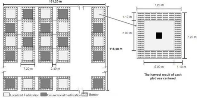
The total area studied (Figure 1) has 1.74 ha, divided into 256 plots of 7.2 m x 7.2 m, with a carrier of 2.4 m in either direction, the data. Half of the plots were managed with localized chemical fertilization (LF) and half with conventional chemical fertilization (CF). The culture was conducted with soybean cultivar CD 201 - conventional soybeans (Coodetec), being grown under the no-tillage system. The harvest was carried out during 1998 to 2002, always in April, using a harvester
developed for experiments in installments. Productivity (t ha-1), adjusted to 13% of water content of
grains, was measured from the mass collected on each parcel from its area. This yield was then associated with its geometric center, following the delineation stratified aligned systematic sampling. The data analyzed in this work were also studied when one of their spatial variability by SOUZA et al. (1999), RACHID JUNIOR et al. (2006) and MILANI et. al. (2006). MILANI et. al. (2006) concluded that the methodology that uses the standard score for normalization of productivity was effective in identifying management zones for the area managed with localized chemical fertilization.
FIGURE 1. Sketch of the research area, showing the stratified aligned systematic sampling.
Position measurements (mean, average and median), dispersion measurements (variance, standard deviation and interquartile range) and shape of the distribution measurements (coefficient of variation, skewness coefficient, and kurtosis coefficient) were calculated during the descriptive
and exploratory data analysis. The variation coefficient (CV) was considered low when CV ≤ 10%
(homoscedasticity), medium when 10% < CV ≤ 20%, high when 20% <CV ≤ 30%, and very high
when CV>30% (heteroscedasticity) (PIMENTEL-GOMES & GARCIA, 2002). The normal distribution of data probability was verified using the tests proposed by Anderson Darling and Kolmogorov-Smirnov, considering normal probability distribution the data that obtained results of p-value greater than 0.05, i.e., at 5% significance level in at least one of the tests. Box-plot graphs
were composed for the verification of points and analysis of discrepant, with the purpose of exclusion after confirmation of inconsistent data.
The structure of spatial variability of the data was verified by geostatistical analysis. To estimate the structure of the experimental semivariance function, it was used the classic Matheron estimator for variables with normality, and the estimator of Cressie and Hawkins, otherwise. The modeling consisted in fitting a theoretical model (spherical, exponential, Gaussian or circular) to the experimental semivariogram, using the estimation method of ordinary least squares, and adopting
the isotropic model (unidirectional semivariogram) with a cutoff of 50% of the maximum distance.
With the most appropriate model, it was found the estimates of the nugget effect parameter (C0),
positions not sampled in the field, by ordinary kriging technique. The spatial dependence rating of the semivariograms was assessed by the nugget effect coefficient (E%, eq. (1), Table 1), used by SOUZA et al. (1999), where E% up to 25% represents a strong spatial dependence, and between 25 and 75% moderate and above 75%, weak spatial dependence.
For the development of management zones, two methods were used to remove the seasonal influence productivity:
1. Normalized productivity method (eq. (2), Table 1): the productivity was divided in each position of the plot by the average yield of the corresponding year (MOORE, 1998; XIANG et al., 2007). After the data normalization, the CV (eq. (3), (4) and (5) of Table 1) was calculated, and then reclassified using the management classes defined in Table 2.
2. Standardized productivity method (eq.(6), (7) and (8), Table 1): Transforming the
productivity in standard score (MILANI et. al., 2006). The problem of the impossibility of calculating the CV of the normalized data by the standard score, as the average of the data is zero was solved by MILANI et. al. (2006), by calculating the CV in terms of unique productivity, which led to CVs values above the reality. This problem was solved here by calculating the equivalent standardized productivity (eq.(9), (10) and (11), Table 1). After the standardization of data, the CV of the equivalent standardized productivity (eq.(2), Table 1) was calculated, and then reclassified using the management classes defined in Table 3.
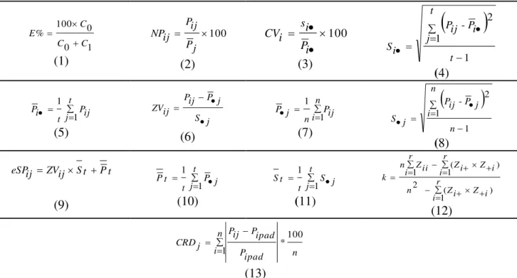
TABLE 1. Equations mentioned in the text.
1 0 0 100 % C C C E (1) 100 j P ij P ij NP (2) 100 i P i s i CV (3)
1 2 -1 t i P ij P t j i S (4) t j Pij t i P 1 1(5) j
S j P ij P ij ZV (6) n i Pij n j P 1 1 (7)
1 2 -1 n j P ij P n i j S (8) t P t S ij ZV ijeSP
(9)
t
j P j t t P 1 1 (10) t
j S j t t S 1 1 (11) r
i Zi Z i n
r
i
r
i Zi Z i ii
Z n k
1( )
2
1 1( )
(12) n n i ipad P ipad P ij P j
CRD *100
1 (13)
Considering: i : 1,2,3...., n ; j : 1, 2 ..., t; E% : nugget effect, PNij : normalized productivity at i point and j year; Pij : average productivity of i point and j year; Pj : average productivity of j year; CVi : variation coefficient at i point and t years; Si: standard deviation of the i point in the t years of study; Pi: average of i point during t years; ZV
ij : standardized productivity at i point and j year; Pj : average productivity of j year; Sj : standard productivity deviation in j year;
eSPij : equivalent standardized productivity of i point in j year; St : average of standard deviation in t years; Pt : average of standard observations in t years;
TABLE 2. Classes of classification (four) of the maps of management zones starting from the normalized productivity (NP) and of the coefficient of variation (CV).
Class NP CV
1 High and consistent NP >105% CV ≤ 30%
2 Average and consistent 95% ≤ NP ≤ 105% CV ≤ 30%
3 Low and consistent NP < 95% CV ≤ 30%
4 Inconsistent - CV > 30%
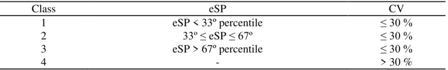
TABLE 3. Classes of classification (four) of the maps of management zones starting from the equivalent standardized productivity (eSP) and of the coefficient of variation (CV).
Class eSP CV
1 eSP < 33º percentile ≤ 30 %
2 33º ≤ eSP ≤ 67º ≤ 30 %
3 eSP > 67º percentile ≤ 30 %
4 - > 30 %
The management zones developed by the two techniques were compared using two methodologies: 1) kappa index (eq.(12), Table 1), and classified according to LANDIS & KOCH (1977, Table 4); 2) Coefficient of relative deviation (CRD, eq. (13), Table 1), proposed by COELHO et al. (2009), using the normalized productivity maps (NP) as a standard.
TABLE 4.Qualitative classification of the kappa index (k).
Quality Terrible Bad Regular Good Very Good Excelent
Kappa index < 0.00 0.01 – 0.20 0.21 – 0.40 0.41 – 0.60 0.61 – 0.80 0.81 – 1.00
Source: LANDIS & KOCH (1977)
RESULTS AND DISCUSSION
The variation coefficients (CV, Table 5) of the soybean productivity with localized fertilization (LF) and conventional fertilization (CF) had a minimum of 12% (LF medium) and 13% (CF, medium), and a maximum of 24% (LF, high) and 36% (CF, very high), classified according to PIMENTEL-GOMES & GARCIA (2002). As expected, the variability was lower for the plots with localized fertilization.
The average productivity was found to be 2.42 t ha-1 for AL and 2.27 t ha-1 for CF, which is
below the period average of 2.48 t ha-1 to Brazil and 2.77 t ha-1 to Paraná (PARANÁ, 2007). It was
only found a normal distribution for the productivity data (with localized fertilization (LF) and conventional fertilization (CF)) for 1998, contributing to the verification of a greater spatial variability.
TABLE 5. Results of the descriptive statistical analysis for the soybean productivity data with localized fertilization (LF) and conventional fertilization (CF), for the years from 1998 to 2002.
Productivity LF (t ha-1) Productivity CF (t ha-1)
1998 1999 2000 2001 2002 1998 1999 2000 2001 2002
Mean 2.71 1.94 3.10 2.61 1.73 2.79 1.96 3.10 2.67 0.84
Average 2.75 2.05 3.16 2.67 1.81 2.70 1.98 3.14 2.75 0.79
CV (%)* 16.2 22.9 12.0 14.7 23.6 19.2 22.9 13.0 13.6 36.4
SD 0.44 0.45 0.37 0.38 0.41 0.54 0.45 0.40 0.36 0.31
Kurtosis 0.21 0.54 1.63 1.25 1.18 -0.12 1.25 1.42 1.87 1.85
Skewness -0.12 -0.81 -1.20 -1.15 -1.16 0.21 -0.80 -1.44 -1.22 1.03
Minimum 1.19 0.69 1.65 1.42 0.45 2.42 1.78 2.92 2.54 0.67
Maximum 3.70 2.81 3.72 3.20 2.34 4.14 2.93 3.98 3.34 1.86
Normality Yes No No No No Yes No No No No
* CV(%) = (SD/average) 100; SD - Standard Deviation
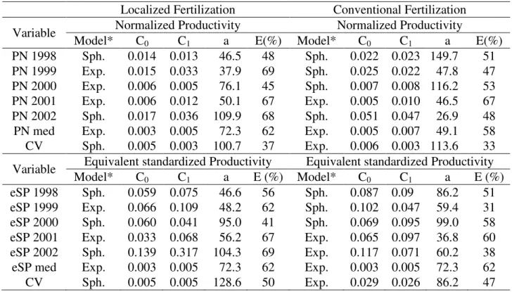
For both systems of fertilization (LF and CF) and both standardization methods (NP and eSP), the adjusted models for the experimental semivariogram were spherical and exponential (Table 6). All data sets showed moderate level of spatial variation as the nugget effect coefficient (E%) was between 25% and 75%. However the average values of E% were 50% to CF and 58% to LF, featuring a smaller spatial dependence for the plots with a localized treatment, as expected.
TABLE 6.Models and parameters of the semivariograms for soybean productivity data, with
localized fertilization and conventional fertilization.
Localized Fertilization Conventional Fertilization
Variable Normalized Productivity Normalized Productivity
Model* C0 C1 a E(%) Model* C0 C1 a E(%)
PN 1998 Sph. 0.014 0.013 46.5 48 Sph. 0.022 0.023 149.7 51
PN 1999 Exp. 0.015 0.033 37.9 69 Sph. 0.025 0.022 47.8 47
PN 2000 Exp. 0.006 0.005 76.1 45 Sph. 0.007 0.008 116.2 53
PN 2001 Exp. 0.006 0.012 50.1 67 Exp. 0.005 0.010 46.5 67
PN 2002 Sph. 0.017 0.036 109.9 68 Sph. 0.051 0.047 26.9 48
PN med Exp. 0.003 0.005 72.3 62 Exp. 0.005 0.007 49.1 58
CV Sph. 0.005 0.003 100.7 37 Exp. 0.006 0.003 113.6 33
Variable Equivalent standardized Productivity Equivalent standardized Productivity
Model* C0 C1 a E (%) Model* C0 C1 a E (%)
eSP 1998 Sph. 0.059 0.075 46.6 56 Sph. 0.087 0.09 86.2 51
eSP 1999 Exp. 0.066 0.109 48.2 62 Sph. 0.102 0.047 59.4 31
eSP 2000 Sph. 0.060 0.041 95.0 41 Sph. 0.069 0.095 99.0 58
eSP 2001 Exp. 0.033 0.068 56.2 67 Exp. 0.065 0.097 36.8 60
eSP 2002 Sph. 0.139 0.317 104.3 69 Exp. 0.117 0.071 60.2 38
eSP med Exp. 0.003 0.005 72.3 62 Exp. 0.003 0.005 72.3 62
CV Sph. 0.005 0.005 128.6 50 Exp. 0.029 0.026 86.2 47
*Model: Sph. - spherical; Exp. - exponential
with conventional fertilization, one can observe differences in the spatial distribution when compared to conventional and localized fertilization.
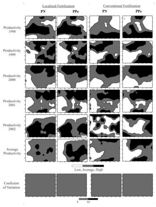
FIGURE 2. Maps of comparison of the normalized productivity (NP) and equivalent standardized
productivity (eSP), with localized and conventional fertilization in the years from 1998 to 2002.
TABLE 7. Coefficient of relative deviation (CRD) and kappa index of agreement for the yield data under the portions with localized fertilization (LF) and conventional fertilization (CF).
Localized Fertilization Convencional Fertilization
Year CRD Kappa CRD Kappa
1998 13.3% 0.78 13.4% 0.79
1999 15.8% 0.75 14.0% 0.78
2000 19.5% 0.70 13.5% 0.81
2001 19.3% 0.70 14.1% 0.78
2002 19.0% 0.71 16.6% 0.73
Average 41.0% 0.32 33.5% 0.49
It was also observed an inverse effect between the CRD and the kappa index (Figure 3), providing a very good correlation, since the provided explanation by the linear model was of 0.99, showing that to make the comparison of maps you can use any of the index studied.
FIGURE 3.Comparison among the values found for the coefficient of relative deviation (CRD) and
for the kappa index.
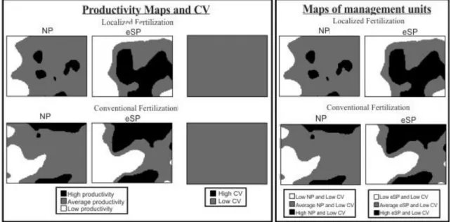
To evaluate the proposed methodologies for the generation of management zones, the sort keys in Table 2 (NP) and Table 3 (eSP) were used. Because the CV in both methodologies has been classified as only one class, the maps of the management zones are coincident of such productivity. (Figure 4).
FIGURE 4.Definition of the management zones starting from the maps of normalized yield (a) and
Because of the different definitions for the classification of normalized productivity, the two methodologies presented variations on the representative area of each class (Table 8). As the contour maps for NP were classified by the percentage from the average, it was found that the representation of classes, shown with different areas (some larger than others), for example, the class with average productivity and low CV featuring 74% (LF) and 67% (CF) of the total area of the map. This did not happen with the eSP because the areas were divided into classes with the same percentage of area (33%).
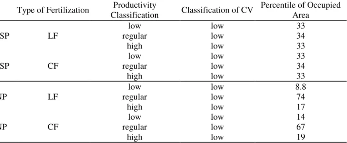
TABELA 8. Percentile of area in each class of classification of the units of management zones, for the contour maps of localized fertilization (LF) and conventional fertilization (CF) starting from normalized productivity (NP) and equivalent standardized productivity (eSP).
Type of Fertilization Productivity
Classification Classification of CV
Percentile of Occupied Area
eSP LF
low low 33
regular low 34
high low 33
eSP CF
low low 33
regular low 34
high low 33
NP LF regular low low low 8.8 74
high low 17
NP CF
low low 14
regular low 67
high low 19
In the comparison of management zones generated by the two methods, it was found through the CRD that, on average, there was a difference of 56% (LF) and 41% (CF) in the module, the interpolated values of normalized productivity in each method. The kappa index allowed us to find the conformity between the management zones considered as good (CF, 0.50) and reasonable (LF, 0.39) (LANDIS & KOCH, 1977).
CONCLUSIONS
The proposed methodology for calculating the equivalent standardized productivity proved effective for permitting, at the same time, the standardization of data using standard score and the variation coefficient (CV) of the variable.
The two methods of management zones definition, using normalized productivity and equivalent standardized productivity, proved to be effective, showing similarities in the arrangement of data. Due to the fact that the equivalent standardized productivity uses score standardized, she has a better statistical justification.
The conformity of the maps was assessed as reasonable for the management zones with plots under conventional fertilization, and good for the management zones with plots under localized fertilization.
REFERENCES
AMADO, T.J.C.; PES, L.Z.; LEMAINSKI, C.L.; SCHENATO, R.B. Atributos químicos e físicos
de latossolos e sua relação com os rendimentos de milho e feijão irrigados. Revista Brasileira de
BLACKMORE, B.S. The interpretation of trends from multiple yield maps. Computers and electronics in agriculture, Amsterdam, v.26, n.2, p.37-51, 2000.
COELHO, E.C.; SOUZA, E.G.; URIBE-OPAZO, M.A.; PINHEIRO NETO, R. Influência da
densidade amostral e do tipo de interpolador na elaboração de mapas temáticos. Acta Scientiarum
Agronomy, Maringá, v.31, n.1, p.165-174, 2009.
DAVIS, G.; CASADY, W.; MASSEY, R. Precision agriculture: an introduction. Water quality.
University of Missouri-System, 1998. p.8. Disponível em:
<https://mospace.umsystem.edu/xmlui/bitstream/handle/10355/9432/PrecisionAgricultureIntroducti on.pdf?sequence=3>. Acesso em: out. 2011.
DOBERMANN, A.; ARKEBAUER, T.; CASSMAN, K.G.; DRIJBER, R.A.; LINDQUIST, J.L.;
SPECHT, J.E. Understanding corn yield potential in different environments. Lincoln: University Of
Nebraska, 2003.
DURIGON, R. Aplicação de técnicas de manejo localizado na cultura do arroz irrigado (Oryza
sativa L.). 2007. 149 f. Dissertação (Mestrado em Engenharia Agrícola) - Universidade Federal de Santa Maria, Santa Maria, 2007.
HORNUNG, A.; KHOSLA, R.; REICH, R.; INMAN, D.; WESTFALL, D.G. Comparison of
site-specific management zones: soil-color-based and yield-based. Agronomy Journal, Madison, v.98,
p.407-415, 2006.
LANDIS, J.; KOCH, G. The measurement of observer agreement for categorical data. Biometrics,
Washington, v.33, n.1, p.159-174, 1977.
MILANI, L.; SOUZA E.G.; URIBE-OPAZO, M.A.; GABRIEL FILHO, A.; JOHANN, J. A.;
PEREIRA J.O. Unidades de manejo a partir de dados de produtividade. Acta Scientiarum
Agronomy, Maringá, v.28, n.4, p.591-598, 2006.
MOORE, M.R. An investigation into the accuracy of yield maps and their subsequent use in crop
management. 1998. 150 f. Thesis (PhD) - Cranfield University, Silsoe, 1998.
PARANÁ (Estado). Secretaria de Estado da Agricultura e do Abastecimento. SOJA. 2007. Boletim Diário. Disponível em: http://www.pr.gov.br/seab/. Acesso em: 23 abr. 2007.
PIMENTEL-GOMES, F.; GARCIA, C. H. Estatística aplicada a experimentos agronômicos e
florestais. Piracicaba: FEALQ. 2002. 307 p.
RACHID JUNIOR, A.; URIBE-OPAZO, M.A.; SOUZA, E.G.; JOHANN, J.A. Variabilidade espacial e temporal de atributos químicos do solo e da produtividade da soja num sistema de
agricultura de precisão. Engenharia na Agricultura, Viçosa-MG, v.14, n.3, p.156-169, 2006.
RODRIGUES JUNIOR, F. A. Geração de zonas de manejo para cafeicultura usando sensor SPAD
e análise foliar. 2008. 64 f. Dissertação (Mestrado em Engenharia Agrícola) - Universidade Federal
de Viçosa, Viçosa, 2008.
SOUZA, E.G.; JOHANN, J.A.; ROCHA, J.V.; RIBEIRO, S.R.A.; SILVA, M.S.; URIBE-OPAZO, M.A.; MOLIN, J.P.; OLIVEIRA, E.F.; NÓBREGA, L.H.P. Variabilidade espacial dos atributos
químicos do solo em um Latossolo roxo Distrófico da região de Cascavel - PR. Engenharia
Agrícola, Jaboticabal, v.18, n3, p.80-92, 1999.
TAYLOR, J.A.; MCBRATNEY, A.B.; WHELAN, B.M. Establishing management classes for
broadacre agricultural production. Agronomy Journal, Madison, v.99, p.1366-1376, 2007.
XIANG, L.; YU-CHUN, P.; ZHONG-QIANG G.; CHUN-JIANG, Z. Delineation and scale effect
of precision agriculture management zones using yield monitor data over four years. Agricultura
YAN, L.; ZHOU, S.; FENG, L.; HONG-YI, L. Delineation of site-specific management zones
using fuzzy clustering analysis in a coastal saline land. Computers and Electronics in Agriculture,
Amsterdam, v.56, p.174-186, 2007.