Analysis of new indicators for fault detection in grid connected PV systems for BIPV applications

DEPARTAMENTO DE ENGENHARIA GEOGRÁFICA, GEOFÍSICA E ENERGIA

Analysis of new indicators for Fault detection in grid

connected PV systems for BIPV applications

Mário Filipe Aires da Silva

Dissertação

Mestrado Integrado em Engenharia da Energia e do Ambiente

DEPARTAMENTO DE ENGENHARIA GEOGRÁFICA, GEOFÍSICA E ENERGIA

Analysis of new indicators for Fault detection in grid

connected PV systems for BIPV applications

Mário Filipe Aires da Silva

Dissertação de Mestrado Integrado em Engenharia da Energia e do Ambiente

Trabalho realizado sob a supervisão de:

Dr. Santiago Silvestre Berges (UPC)

Dr. Miguel Centeno Brito (FCUL)

I would like to thank to everyone who contributed in one way or another to the successful accomplishment of this thesis, but in particular I would like to thank to:

Supervisor Professor Miguel Centeno Brito for his availability and collaboration before and during this work;

Co-supervisor Professor Santiago Silvestre Berges for his good orientation and help during this work. I am also grateful the good way he received me in Polytechnic University of Catalunya (UPC).

Doctor Daniel Guasch Murillo for his availability and help with the understanding of his MatLab models.

Carolina Pires for her important support during the execution of this thesis. My friend Engineer Arturo Marban for his help with MatLab when I most needed.

Finally, I am grateful to my parents, Mário and Paula, my brother Bruno and my grand-parents, Horácio and Clotilde, for their support and the strength they gave me during my academic path and my staying in Barcelona.

Abstract

In this work we present a new procedure for automatic fault detection in grid connected photovoltaic (PV) systems. Most diagnostic methods for fault detection of PV systems already known are time consuming and need expensive hardware. In order to completely avoid the use of modeling and simulation of the PV system in the fault detection procedure we defined two new current and voltage indicators, NRc and NRv respectively, in the DC side of the inverter of the PV system. This method is based on the evaluation of these indicators. Thresholds for these indicators are defined taking into account the PV system configuration: Number of PV modules included in series and parallel interconnection to form the PV array. The definition of these thresholds for the voltage and current indicators must be adapted to the specific PV system to supervise and a training period is recommended to ensure a correct diagnosis and reduce the probability of false faults detected. A simulation study was carried using MatLab and the data used was monitored by the inverter, pyranometers, thermocouples and reference cells installed in a grid connected PV system located in the Centre de Développement des Energies Renouvelables (CDER), Algeria. The proposed method is simple but effective detecting the main faults of a PV system and was experimentally validated and has demonstrated its effectiveness in the detection of main faults present in grid connected applications.

Key word: Photovoltaic Energy, PV systems, Fault Detection, Diagnosis of Faults, New

Resumo

Neste trabalho apresentamos um novo procedimento para deteção automática de falhas em sistemas fotovoltaicos (PV) ligados à rede. A maioria dos métodos de diagnóstico para deteção de falhas em sistemas PV já conhecidos são consumidores de tempo e precisam de equipamento caro. De forma a evitar completamente o uso de modelação e simulação do sistema PV no processo de deteção de falhas, nós definimos dois novos indicadores de corrente e voltagem, NRc e NRv, respetivamente, no lado DC do inversor do sistema PV. Este método é baseado na avaliação desses novos indicadores. Foram definidos limites para esses indicadores de forma a ter em conta a configuração do sistema PV: número de módulos PV incluídos em série e em paralelo que formam o PV array. A definição desses limites para os indicadores de voltagem e corrente têm que ser adaptados ao sistema PV específico a supervisionar e um período de treino é recomendado de forma a garantir um diagnóstico correto e reduzir assim a probabilidade de falsas falhas detetadas. Um estudo de simulações foi feito em MatLab e usando informação monitorizada pelo inversor, piranómetros, termopares e células de referência instaladas no sistema PV conectado à rede localizado no Centro de Desenvolvimento das Energias Renováveis (CDER), Algéria. O método proposto é simples mas eficaz na deteção das falhas principais de um sistema PV e foi experimentalmente validado e demonstrou a sua eficácia na deteção de falhas presentes em aplicações conectadas à rede.

Palavras-chave: Energia Fotovoltaica, Sistemas PV, Deteção de Falhas, Diagnóstico de Falhas,

1. Introduction ... 1

1.1 Motivations ... 1

1.2 Outline of the thesis ... 2

1.3 Solar cell & PV module ... 3

1.4 The I-V curves ... 5

1.4.1 Scaling I-V curve ... 5

1.4.2 Impacts of Temperature and Irradiance on the I-V curve ... 6

1.5 Power curves & MPP ... 8

1.6 Photovoltaic systems configurations ... 11

1.6.1 Stand-alone PV systems ... 11

1.6.2 Grid connected PV systems ... 11

1.7 Components of grid connected photovoltaic systems ... 12

1.8 Common faults and degradation factors ... 15

1.9 O&M practice ... 17

2. State of the art ... 19

2.1 Monitoring systems ... 19

2.2 Fault detection & diagnosis ... 20

2.3 Review of Chouder’s procedure ... 21

2.3.1 Description of the PV system installed at CDER and the monitoring system ... 21

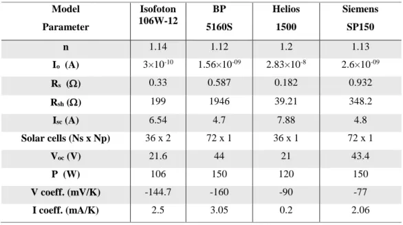
2.3.2 PV module Parameters extraction ... 23

2.3.3 Fault Diagnosis based on energy yields, current and voltage indicators ... 24

2.3.4 Power loss factors in PV systems ... 24

2.3.5 Indicators for failure detection ... 29

3. New Indicators for Fault Detection and Diagnosis of PV Systems ... 31

3.1 Soft environment & MatLab ... 31

3.2 New I&V indicators ... 32

3.2.1 New Indicators, NRc and NRv ... 32

3.2.2 Calculation of Iscm and Vocm (PV Module) ... 32

3.2.3 Calculation of Imm and Vmm (PV Module) ... 35

3.2.4 Calculation of Isc and Voc (Array) ... 37

3.2.5 Indicators in Fault-Free operation ... 37

3.3 Faults on PV systems ... 38

3.3.1 Fault detection ... 38

3.4.2 Simulated systems ... 43

3.4.3 Indicators values for the simulations of all systems ... 45

3.4.4 Obtaining  and  by using both procedures... 45

3.5 Impacts of string faults and short-circuited modules ... 47

3.5.1 Impacts of faulty strings ... 47

3.5.2 Impacts of short-circuited PV modules ... 50

3.5.3 Impacts on the output Power ... 52

4. Experimental Validation ... 56

4.1 System Behavior ... 56

4.1.1 Case of study 1: Free Fault ... 57

4.1.2 Case of study 2: String Fault ... 59

4.1.3 Case of study 3: Short-circuited PV modules ... 62

4.2 Detection and diagnose of changing energy loss type of failures ... 64

4.2.1 Partial Shadowing ... 64

4.2.2 Grid Fault ... 68

5. Conclusions ... 73

6. Annex ... 74

PV Photovoltaic

NRc New Ratio of Current

NRv New Ratio of Voltage

CDER Centre de Développement des Energies Renouvelables

η Efficiency

G Irradiance

I-V Current-Voltage curve

Ns Number of cells/modules connected in series

Np Number of cells/modules connected in parallel

STC Standard Test Conditions

MPP Maximum Power Point

MPPT Maximum Power Point Tracker

FF Fill Factor

Si Silicon

DC Direct Current

AC Alternate Current

O&M Operating & Maintenance

IEA International Energy Agency

Yr Reference Yield

Ya Array Yield

Yf Final Yield

PR Performance Ratio

Vm Voltage at Maximum Power Point

Im Current at Maximum Power Point

NRvbm New Ratio of Voltage with short-circuited module NRcfs New Ratio of Current with faulty string

TNRcfs Threshold of faulty string fault

TNRvbm Threshold of short-circuited module fault

Fig. 1.1- Typical silicon solar cell ... 3

Fig. 1.2- Schematic of a solar cell connected to a load ... 3

Fig. 1.3- Typical Silicon PV module ... 4

Fig. 1.4- Cells connected in series with bypassed diodes ... 4

Fig. 1.5- Simulated I-V curve for one solar cell of the PV module Isofoton 106/12, at STC ... 5

Fig. 1.6- Scaling the I-V curve from a solar cell to a PV array ... 6

Fig. 1.7- Simulated I-V curve for the PV module Isofoton 106/12, at STC ... 6

Fig. 1.8- Effect of Diverging Rs & Rsh from Ideality ... 7

Fig. 1.9- Effect of the Irradiance (G) on the I-V curve at 25°C ... 7

Fig. 1.10- Effect of the Cell Temperature (Tcell) on the I-V curve at 1000 W/m2 _{... 8}

Fig. 1.11- Typical I-V curve including P-V curve for a random PV module ... 9

Fig. 1.12- Effect of the Irradiance (G) on the Power curve and MPP, at 25°C ... 10

Fig. 1.13- Effect of Tcell on the Power curve and MPP, at 1000 W/m2_{... 10}

Fig. 1.14- Standard configuration of a Stand-alone PV system ... 11

Fig. 1.15- Standard configuration of a Grid connected PV system ... 12

Fig. 1.16- Common PV Inverter - Sunny Boy 2500HF ... 13

Fig. 1.17- Junction box... 14

Fig. 1.18- Pyranometers on the tilted and horizontal planes ... 14

Fig. 1.19- Cleaning the soiling in a PV array ... 16

Fig. 1.20- Snow covering PV modules ... 17

Fig. 1.21- Partial shading... 17

Fig. 2.1- General Scheme of the PV system installed in CDER ... 22

Fig. 2.2- Monitoring system installed at CDER ... 22

Fig. 2.3- PV system output Power, DC side – measured and simulated ... 23

Fig. 2.4- Loss mechanisms in PV systems ... 26

Fig. 2.5- Capture losses evolution on free fault operation of the PV system ... 28

Fig. 2.6- Capture losses evolution on faulty string operation of the PV system ... 29

Fig. 2.7- Most probable faults present in the PV system ... 30

Fig. 3.1- I-V curves with G=1000 W/m2_{, BP 5160S ... 34}

Fig. 3.2- I-V curves with G=1000 W/m2_{, Helios 1500 ... 34}

Fig. 3.3- Power curve - BP BP5160S ... 36

Fig. 3.4- Power curve – Helios 1500 ... 36

Fig. 3.5- Model for detection of both faults: short-circuited modules and faulty strings ... 42

Fig. 3.6- Common scheme of a grid connected PV system ... 44

Fig. 3.7-  parameter values as a function of Np ... 46

Fig. 3.8-  parameter values as a function of Ns ... 47

Fig. 3.9- Output Current profile with different number of faulty strings... 48

Fig. 3.10- NRc: Current ratio profiles ... 48

Fig. 3.11- Power profile with different number of faulty strings ... 49

Fig. 3.12 Voltage profile with different number of short-circuited modules ... 50

Fig. 3.13- NRv: Voltage ratio profile ... 51

Fig. 3.14- Power profile with different number short-circuited modules ... 52

Fig. 3.15- NRv progression – PV system number 3 ... 53

Fig. 4.4- Ratios and threshold for output voltage – Free fault ... 58

Fig. 4.5- Irradiance profile – string fault day ... 59

Fig. 4.6- Cell Temperature profile – String fault day ... 60

Fig. 4.7- Ratios and threshold for output current – String fault ... 60

Fig. 4.8- Ratios and threshold for output voltage – String fault ... 61

Fig. 4.9- Irradiance profile – Short-circuited module day ... 62

Fig. 4.10- Cell Temperature profile – Short-circuited module day ... 62

Fig. 4.11- Ratios and threshold for output Voltage – Short-circuited PV module ... 63

Fig. 4.12- Ratios and threshold for output Current – Short-circuited PV module ... 63

Fig. 4.13- Irradiance profile with Shading ... 65

Fig. 4.14- Cell Temperature profile with Shading ... 65

Fig. 4.15- Current profile at DC side of the PV system with Shading ... 66

Fig. 4.16- Voltage profile at DC side of the PV system with Shading... 66

Fig. 4.17- Power profile at the DC side with Shading ... 67

Fig. 4.18- NRc profile with Shading ... 67

Fig. 4.19- NRv profile with Shading ... 68

Fig. 4.20- Irradiance profile with Shading ... 69

Fig. 4.21- Cell Temperature profile with Shading ... 69

Fig. 4.22- Current profile at DC side of the PV system with Shading and Grid faults ... 70

Fig. 4.23- Voltage profile at DC side of the PV system with Shading and Grid Faults ... 70

Fig. 4.24- Power profile at DC side of the PV system with Shading and Grid Faults ... 71

Fig. 4.25- NRc profile with Shading and Grid Faults ... 71

Table 2.1- Typical monitoring inputs in a common PV system [23] ... 19

Table 3.1- Commercial PV modules used on this work ... 33

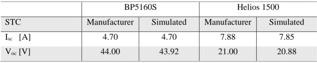
Table 3.2- Isc and Voc results from manufacturer and simulated data ... 35

Table 3.3- Vmpp, Impp and Pmpp results from manufacturer and simulated data ... 37

Table 3.4- Constant Energy Loss Faults in a PV system based on the new indicators ... 39

Table 3.5- Systems of study configuration... 44

Table 3.6- Results from all the system simulations ... 45

Table 3.7- Values obtained for  and  ... 46

Table 4.1- Ratios and thresholds values – free fault ... 59

Table 4.2- Ratios and thresholds values – String fault ... 61

1. Introduction

1.1

Motivations

Due to technology developments and to a considerable demographic grown, it has been verified from decade to decade an increased consumption of energy all over the world. If there are no changes or set new laws that may affect energy markets, the consumption of energy will keep increasing. A large piece of this increase is due to fossil fuels. Unfortunately, fossil fuels are considered finite and limited resources and are the main sources of air pollution and green house effect.

Renewable energy seems to be the best alternative to fossil fuels. This kind of energy has many benefits like helping to keep the air clean, reduce the dependence on fossil fuels, reduce the production of carbon dioxide, create new jobs and create sustainable development of the countries. Wind energy, hydroelectric generation, biomass, geothermal, photovoltaic, solar thermal energy are all examples of renewable energies.

In the last few years, there was a huge grown of the number of photovoltaic systems installed all over the world. This happens thanks to the reduction of the PV modules fabrication cost and the policies adopted by most of the countries in the world that give some benefits and new fees to whom have those systems installed at home. However, this growth has not been accompanied by important improvements in the field of PV system diagnosis, supervision and fault detection [3] because it is a common belief that PV systems are maintenance free and monitoring PV systems represent an extra cost. Even if a PV panel shows a really low failure rate, it is important to keep in mind that PV systems are composed by other elements that may also have failures. Also, faults in PV systems do not only affect the performance of the system but may also lead to damage the equipment. Moreover, although PV systems generally operate without problems, when there are faults on the system they are hard to be observed by the operating personnel. In order to prevent faults and failures that lead to a decrease of the lifetime of a PV system, and to improve the system efficiency, monitoring and fault detection have to be practiced.

The fault detection procedure presented in this thesis work is based on previous works that evaluate the power losses present in the PV system for fault detection [4-6,30]. In this approach the computational analysis has been reduced avoiding the use of electrical models for simulation of the PV system behavior and the number of monitoring sensors minimized.

Nowadays most inverters designed for grid connected PV applications have a wide range of interfaces, in particular sensor inputs and communication interfaces. These sensor inputs can be used to connect irradiance sensors as pyranometers, reference cells and PV module temperature sensors. So, these inverters include monitoring capabilities for irradiance and temperature as well as for maximum power point tracking (MPPT) evolution. The proposed method uses as input variables from the inverter just the DC currents and voltages extracted from the MPPT incorporated in the inverter, the measured irradiance and cell temperature.

Therefore, this thesis work aims to develop a method of fault detection that can be integrated into the inverter without using simulation software or additional external hardware. The focus of this work is the losses and malfunction of the DC side. Two new indicators of current and voltage are used as benchmarks and both relationships can be calculated by the inverter himself.

1.2

Outline of the thesis

This thesis consists in six chapters, with the first chapter giving a little introduction to the theme of solar energy. Afterwards an overview on how the solar energy production works explaining the solar cell and PV modules concept. Then the I-V curve, Power curve and maximum power point (MPP) are introduced with the impacts of various factors that may change these indicators. Following this, the photovoltaic (PV) system itself is introduced distinguishing characteristics of the two main types of PV systems, stand-alone and grid connected PV systems. Ending this chapter we have an overview of the components of a grid connected PV system, the common faults and degradations factors, and finally the O&M.

Chapter 2 will start with the state of the art of monitoring systems used on PV systems and methods of detection and diagnosis of faults recently developed. Afterwards, will be given a review of the Chouder’s work we based our new method. In this review we have a detailed explanation of the actual grid connected PV system located in the Centre de Développement des Energies Renouvelables (CDER) in Algeria, simulated and measured and an overview of the method used for the parameter extraction (Rsh, Rs, n, I0, IPH). Then we introduce the energy yields and the capture losses because this

is the basis of the previous work of fault detection and diagnosis in PV systems. In the end of this chapter there are some results in order to better understand this method and most importantly the previous indicators reported in the literature that were the basis of the work developed in this thesis. In chapter 3 will start with the software used in this thesis. After will be introduced the new indicators of current and voltage, NRc and NRv respectively. Afterwards, we will explain and define the variables that are related to the new indicators and then we will define the NRco and NRvo that are always the expected values in free fault operation of a PV system. Then will be described the different faults and the thresholds related to them and we are going to define the variables α and β used in the definition of the thresholds. After that we have simulations and results based in the new indicators and on the MatLab models. Ending this chapter, there is a study on the impacts of the short-circuited modules and string faults in the output power of a common PV system.

Chapter 4 is dedicated to the system validation where we simulate a sub-array of the actual PV system installed at CDER with actual monitored data and where are presented the results of fault detection and fault diagnosis with the new indicators, NRc and NRv.

1.3

Solar cell & PV module

Fig. 1.1- Typical silicon solar cell

In order to better understand how a PV module works we have to start by the solar cell. A solar cell can be described as an electronic device able to capture the energy of the photons and directly convert it to electricity. Here the process is briefly described considering a crystal silicon cell, the cells used on this thesis. Figure 1.2 shows a simple circuit of a silicon solar cell with an external load:

Fig. 1.2- Schematic of a solar cell connected to a load

The generation of current in a solar cell is known as the “light-generated current”. When a photon is absorbed by the cell, if its energy is greater than the band gap, an electron is able to jump out in the crystal structure creating a hole-electron pair, which normally disappears as the electron recombines with the hole. In order to avoid the recombination a barrier is created by doping the silicon, on one side with small amount of a group III element (for ex. Boron) to form p-silicon and on the other side with a small amount of a group V element (for ex. Phosphorus) to form the n-silicon. The presence of the barrier does not allow the recombination, creating an excess of electrons in the n-silicon and a lack of them in the p-silicon. If an external electrical circuit is built the electrons are free to move from the n-silicon to the p-silicon passing by the electrical circuit, thus producing electricity. This is the basic principle behind the solar cell. Depending on the environmental conditions, mainly the irradiation and the temperature, the cell is able to produce a certain voltage and a certain current [7]. This process is just briefly described because this is not the main focus of this thesis is the PV system.

Fig. 1.3- Typical Silicon PV module

Therefore, a PV module is an aggregate of solar cells connected and grouped. Usually, the solar cells are connected only in series in order to increase the overall output voltage of the PV module but sometimes they also have one connection in parallel in order to increase the overall output current and when that happens the PV module has 2 internal strings of connected solar cells. The same current flows in every cell of the modules and the overall voltage generated is the sum of the voltage of every cell. Due to the fact that the cells are connected in series, the damage of one of them could affect the performance of the entire panel because the current flowing in the cells is the same and its values will adjust to the worst cell in the panel. Furthermore, if one cell of the panel is shaded, it is going to behave as a resistance, i.e. dissipating the electrical energy as heat. This effect is called hot spot. Hot spot is the increase in temperature due to the heat that will damage the solar cell in time. In order to avoid this effect, it is a common practice to introduce in the module by-pass diodes that give to the current an alternative path [8].

Fig. 1.4- Cells connected in series with bypassed diodes

The efficiency of the PV module is expressed as the ratio between the incident power of the solar radiation by the power produced by the module. Thus, the efficiency takes into account all the losses of the system:

𝜂 =𝑉𝑚𝑝∗𝐼𝑚𝑝

𝐺∗𝐴 (1.1)

Where G is the incident irradiance [W/m2_{]; A is the area of the module [m}2_{]; V}

mp is the maximum

power point voltage [V]; Imp is the maximum power point current [A]. The losses will be explained in

the section 1.8.

1.4

The I-V curves

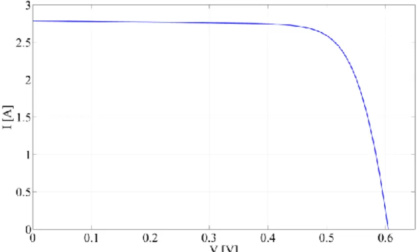
The current-voltage relationship characteristic of a solar cell is typically analyzed with the I-V curve. Figure 1.5 shows us a solar cell I-V curve under predefined environmental conditions:

Fig. 1.5- Simulated I-V curve for one solar cell of the PV module Isofoton 106/12, at STC

The typical I-V curve of an illuminated PV cell has the shape shown in Figure 1.5. The voltage is always represented on the x-axis and current on the y-axis. The short circuit current (Isc) is shown by

the point in which the curve meets the y-axis, this means that in case of short circuit current the voltage is equal to zero. In the other hand, the similar happens with the open circuit voltage (Voc), in

this case the current is equal to zero.

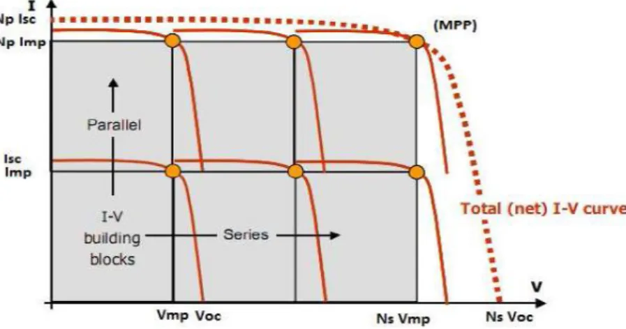
1.4.1 Scaling I-V curve

The I-V curve of a PV array is a scale-up of the I-V curve of a single cell as shown in Figure 1.6. For example, if a PV module has 36 series-connected cells and a PV string has 10 of these modules in series, then the string’s Voc (voltage in open circuit) and also the array’s Voc is 360 times the voltage of

that single solar cell. Similar logic applies to the Isc (short circuit current), which scales with the

number of cells in parallel. Therefore, the maximum power point (MPP) scales too. MPP will be explained in the section 1.5.

Fig. 1.6- Scaling the I-V curve from a solar cell to a PV array

Thus, from now on, the following graphs and explanations will be related to PV modules. Figure 1.7 shows the I-V curve of the PV module Isofoton 106/12 that has Ns=36 cells and Np=2 cells, totaling 72 solar cells.

Fig. 1.7- Simulated I-V curve for the PV module Isofoton 106/12, at STC

1.4.2 Impacts of Temperature and Irradiance on the I-V curve

The I-V curve shown in Figure 1.7 is related to standard test conditions (STC: T=25ºC, G=1000W/m2_{). Sometimes I-V curves may change. Those changes might occur when the following 4}

parameters change: shunt resistances (Rsh), series resistances (Rs), irradiance (G), temperature of the

solar cell (Tcell). The first two parameters are related to the solar cells/PV modules characteristics and the last two are external parameters. Usually the changes related to the resistances are not that great but as we can see in the Figure 1.8 the variations of Rs and Rsh may affect the I-V curve and then affect

Fig. 1.8- Effect of Diverging Rs & Rsh from Ideality

The variations on the two external parameters, G and Tcell, change the I-V curve, in a slightly different way, but with a more important impact of the I-V curve. Figures 1.9 and 1.10 shows the impact of variations of G and Tcell, respectively, on the I-V curve of a PV module:

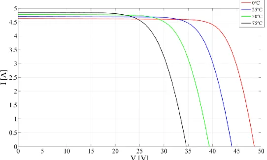
Fig. 1.10- Effect of the Cell Temperature (Tcell) on the I-V curve at 1000 W/m2

With Figure 1.9 and 1.10 we can have some conclusions about how these external factors change the I-V curve. When the irradiance is lower, the variations are more notorious on the output current of the PV module but still there are some decreases on voltage output too when lowering the irradiance. Analyzing the temperature effects, we can see that the variations are more notorious on the output voltage of the module and there are almost no changes on the output current. Therefore, with lower temperatures of the solar cells we might have a bigger MPP thus increasing the output power from the PV module. Comparing the impacts of Rs, Rsh, G and Tcell on the I-V curve, can be concluded that

low values of irradiance have the biggest impact on the I-V curve comparing with the other three model parameters.

1.5

Power curves & MPP

In order to maximize the energy generation of the PV module it is essential that the solar panel works at the maximum power point (MPP) and that’s why the need of using a maximum power point tracker (MPPT). This device will be described in detail in the section 1.7.

The output power of a PV module is the product of the output current delivered to the electric load and the voltage across the module. The value of the power at the Isc point is zero, because the voltage is

zero, and also the power is zero at the Voc point where the current is zero. The maximum output power

of the PV module is somewhere in between. This happens at a point called the maximum power point (MPP) with the coordinates V = Vm and I = Im [9].

As the output power of the PV module is the product between the current and the voltage, it is then possible to draw also the power curve as it can be seen from Figure 1.11:

Fig. 1.11- Typical I-V curve including P-V curve for a random PV module

Another important parameter of PV modules is the fill factor, which is used for the evaluation of the PV module performance:

𝐹𝐹 =𝑉𝑚𝑝∗𝐼𝑚𝑝

𝑉𝑜𝑐∗𝐼𝑠𝑐 (1.2)

Where Voc is the open circuit voltage [V] and Isc is the short-circuit current [A].

The fill factor is a parameter which, in conjunction with Voc and Isc, determines the maximum power

from a solar cell/module. Graphically, the FF is a measure of the "squareness" [10] of the solar cell and is also the area of the largest rectangle which will fit in the IV curve, as can be seen in Figure 1.11. Therefore, a higher FF means a higher module performance.

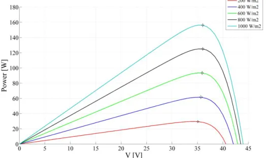
The external parameters, G and Tcell, impact the Power curve. Figure 1.12 shows the impact of different irradiances on the Power curve of a PV module:

Fig. 1.12- Effect of the Irradiance (G) on the Power curve and MPP, at 25°C

Figure 1.13 shows the impact of the cell temperature (Tcell) on the Power curve of a PV module:

Fig. 1.13- Effect of Tcell on the Power curve and MPP, at 1000 W/m2

With figure 1.12 and 1.13 we can have some conclusions about how these external factors may change the Power curve. The impact of G and Tcell on the Power curve is very similar to the impact on the I-V curve, already explained before. What we now realize with these Power curves is that the Tcell has a bigger impact on the output Power than we realized before, after analyzing the I-V curves. Therefore, with lower temperatures of the solar cells and with high irradiance we have a bigger MPP, thus increasing the generated energy from the PV module.

1.6

Photovoltaic systems configurations

Photovoltaic (PV) systems are mainly defined based on if the energy generated by the system is stored or it is directly connected to the grid. Thus, there are stand-alone PV systems and grid connected PV systems [11,12].

1.6.1 Stand-alone PV systems

Stand-alone PV systems are the most popular system used worldwide despite the more recent interest of the market in grid connected PV systems. A stand-alone PV system should provide enough energy to a totally main-isolated application. The standard configuration of this system is shown in Figure 1.14. In some specific cases, such as water pumping, the generator can be connected directly to the motor [13].The range of applications is constantly growing. Mini-applications such as pocket calculators, clocks are well known examples of stand-alone systems. Other typical applications for stand-alone systems are mobile systems on cars, village electrification in developing countries, solar pump systems for drinking water and irrigation, etc [11,12].

Fig. 1.14- Standard configuration of a Stand-alone PV system

Rechargeable batteries are used to store the electricity. In order to protect them, to achieve a higher availability and to have a longer lifetime it is essential the use of a charge controller. The charge controller prevents overcharging and may prevent against overvoltage of the battery.

1.6.2 Grid connected PV systems

In the last few years an important growth of grid-connected PV systems has been observed, especially in industrialized countries. Several reasons lie behind this fact apart from traditional advantages of photovoltaic electricity [14]:

 Utility grid-interactive PV systems are becoming more economically viable as the cost of PV components has been significantly decreasing in recent years, in particular the average cost of PV modules and inverters.

 Technical issues associated with inverters and interconnections of PV systems to the grid have been addressed by manufacturers and today’s generation of inverters has enhanced reliability and reduced size.

 Utility benefits. The fact that solar electricity is produced in central hours of the day can add value to the electricity. This power peak demand can be partially supplied by dispersed grid-connected PV systems that are able to generate power at the same place where this power is used, reducing the heavy load supported by the transmission systems and achieving benefits in distribution and line support.

This market is becoming more and more important in photovoltaic applications. Therefore, PV power generation systems are likely to become, although small compared with other power generation sources, important sources of distributed generation, interconnected with utility grids [14].

Fig. 1.15- Standard configuration of a Grid connected PV system

1.7

Components of grid connected photovoltaic systems

A PV system is more than a mere solar panel. These systems need a lot more components in order to be complete and working. Some of those components are optional and used only for certain occasions. As this new method is based in a grid connected PV system, we are not explaining certain components that are used only in stand-alone systems because they are irrelevant for our present work. Thus, this section aims to give an overview of the different components of a grid connected PV system, which are the following:

 PV modules;  Junction box;  Fuses box;  Wiring;  Inverter;  MPPT;

 Temperature sensor (optional);

 Reference solar cell (optional);

 Pyranometer (optional);

 Device for data acquisition (optional);

 Utility meter (or bidirectional meters);

 Transformer (or isolation transformer).

The main component of a PV system is the photovoltaic module. A PV system is composed by PV modules that can be connected in series or in parallel. The solar cells that compose that PV module can be connected in series or in parallel too. The difference between a connection in series or in

parallel for both, cells or modules, is that the connection in series will increase the overall voltage output, while the connection in parallel will increase the overall current output. More about how the PV modules works is in a previous section. There are PV modules based in multijunction cells, single-juntion GaAs, Cystaline Si (silicon) cells, thin-film technologies (usually cadmium telluride - CdTe) and some emerging technologies like organic cells and more. Actually, the most common cells used in PV modules are crystalline Si cells because it’s a mature technology that allows the best relation between production costs and energy generated. In this thesis, the simulations and all the work done is based in PV systems with silicon based PV modules.

The planning of a grid-connected PV system begins with the choice of an inverter. This determinates the system voltage at the DC side, and then the solar generator can be configured according to the input characteristics of the solar inverter. The inverter is the second most important component in a grid-connected PV system, after the solar generator. Its task is to convert the direct current generated by the solar cells to a 50 Hz AC current required by the grid [15].

Fig. 1.16- Common PV Inverter - Sunny Boy 2500HF

Usually, the inverter also includes components that are responsible for the daily operation mode. During the day, the optimum working point on the I-V characteristic curve shifts according to the fluctuations in solar radiation and module temperature. Intelligent inverter control includes maximum power point (MPP) tracking and continuous readjustment to the most favorable working point. As previously described, it is important that all the modules work at the maximum power point. This point is not fixed in real time because of the variations of external environmental conditions as for example the most common: temperature and irradiation. That is why it is important to track the maximum power point in real time, as explained in a previous section. In order to track this point a maximum power point tracking (MPPT) element is required to vary the output voltage of the string by maximizing the generated power in any real operating conditions [16]. Actually MPPT capabilities are usually included in the inverters used in grid connected PV systems. However, if inverters without MPPT are used, the MPPT algorithm can be separately incorporated into the system by means of DC-DC converters between the output of the PV array and the inverter input. The ideal PV system would have an individual MPPT on every PV module and that’s why there are micro inverters. The presence of more than one MPPT permits better performance of the entire PV system but the costs would rise too much. Therefore, nowadays is not common to see MPPT on every module of a PV system.

Fig. 1.17- Junction box

It is common to use junction boxes, as can be seen in Fig.1.17, on every PV module in order to connect them all together, which contains also bypass diodes. However, nowadays the modules already have bypass diodes incorporated hence the junction box is usually used only to connect them. One damaged module can greatly affect the output power and then the overall energy generation of the entire system. Usually, this happens when hot-spot heating occurs. If the operating current of the overall series string approaches the short-circuit current of the "bad" cell, the overall current becomes limited by the bad cell. The extra current produced by the good cells then forward biases the good solar cells. If the series string is short circuited, then the forward bias across all of these cells reverse biases the shaded cell. Hot-spot heating occurs when a large number of series connected cells cause a large reverse bias across the shaded cell, leading to large dissipation of power in the shaded cell. Essentially the entire generating capacity of all the good cells is dissipated in the shaded cell. The enormous power dissipation occurring in a small area results in local overheating, or "hot-spots", which in turn leads to destructive effects, such as cell or glass cracking, melting of solder or degradation of the solar cell [10]. Therefore, a bypass diode is connected in parallel, but with opposite polarity. The presence of the bypass diode allows the current to follow another path bypassing the damaged solar cell or PV module. In practice, one bypass diode per solar cell is too expensive so bypass diodes are usually placed across groups of solar cells in order to decrease the final costs of the module.

Fig. 1.18- Pyranometers on the tilted and horizontal planes

Another component of a PV system is the temperature sensor, the reference solar cell and the pyranometer. The first one is used to measure the temperature of the air near the PV plant and the temperature at the cell level. Then we have the reference solar cell that enables a high level of measurement precision and is usually used to measure the irradiance that reaches the PV modules at the horizontal plane. Then the pyranometer is also used to measure the irradiance. This device can measure irradiance in both, tilted plane and in the horizontal plane. These three components are optional but they were used on the PV plant in study in order to get the data we needed for our simulations.

Usually, bi-directional meters are needed in grid connected PV systems in order to get the return credits from the energy companies because of the energy fees. Thus, a bi-directional meter records and measure the electricity flowing two ways, i.e. both the electricity drawn from the grid and the excess electricity the PV system feeds back into the grid [17].

Isolation transformers can be optionally placed at the inverter output depending on the type of inverter used in the PV system. Some inverters already include transformers of this type incorporated inside while others do not. An isolation transformer is preferably installed on the AC side of the PV inverter to eliminate the possibility of PV system injecting direct current into the power grid [18]. Some national regulations require an isolation transformer for connection to grids of medium, high or very high voltage. In most countries this is not required for low voltage connection [14].

Finally, in order to monitor all the data given by the sensors present in the system we need a monitoring device. In the PV plant in study, an Agilent 34970A was used for the data acquisition and then the data is sent to a PC via GPIB.

1.8

Common faults and degradation factors

While PV systems have no moving parts (compared to wind and micro-hydro systems) and can be extremely reliable, it does not mean they do not have potential performance problems [19]. Field surveys and inspections, like the survey of residential PV systems in Australia [20] and in Japan [3], show that a significant percentage of PV systems experience faults. For this analysis it is convenient to divide a PV system in three different parts: AC side, DC side and the inverter.

If a failure is registered on the AC side, the possible cause might be grid instability or a problem on the connections between inverter, load and grid. The grid failure is highly related and dependent to the location considered. The probability of grid fault is higher in rural areas while it has lower probability of happening in urban and more industrialized countries with a more stable grid.

Internal errors of the inverter are a common fault in PV systems and they increase with the aging of the component. They can be related with the components of the inverter itself such as switches, the MPPT, the fan or the varistors. However, the inverter has been improved considerably in the last few years in order to increase his reliability.

The DC side usually represents the lower amount of faults but this is the part of the system that raises more difficulties for fault detection and diagnosis of faults [12].

Based on several scientific papers [21], it was possible then to identify the most common faults in a PV system, displayed here from the one with higher probability to the one with the lower:

 Internal error of the inverter: Internal errors can be generated for different reasons and the fault detection system of the own inverter is normally able to identify them and send an error code. The probability of faults related to the inverter is decreasing significantly because they have been improved a lot in the last few years.

 Failures of the data acquisition system: Happens due to problems with the wires and wireless connection, damage of measurement components like the reference cell or the pyranometer.

 Grid instability: This kind of fault is dependent on the grid quality of the location where the PV system is installed. This fault has higher probability of happening in rural areas. This fault might cause unintentional Islanding that causes a continued energizing of the load after the disconnection from the grid and might be dangerous for the O&M technicians.

 Short circuit with the Ground: This happens when there is a short circuit evolving the system and the ground.

 Broken cells: This might occurs due to the accidental impact of objects on PV modules or due to hot spot.

 Aging of PV modules: PV modules are the most durable components in a PV system but they get older as every other component. The average annual degradation of a crystalline silicon module is approximately 0.2% per year, having an impact on the Isc and then on the output

power [3].

 Shading: Periodic shading cannot be considered a fault but is a cause of the decrease of generated energy. Modules affected by shadows get further deterioration due the hot spots as explained before.

Therefore, we can divide failures by their effect in terms of energy loss:

 Constant energy loss type of failure:

o Degradation of the cell; o Short-circuited PV module;

o Module defect;

o Soiling.

Fig. 1.19- Cleaning the soiling in a PV array

 Changing energy loss type of failure:

o Shading;

o Grid failure;

o MPPT errors;

o Snow cover;

Fig. 1.20- Snow covering PV modules

Fig. 1.21- Partial shading

1.9

O&M practice

Usually, PV companies offer a monitoring system but none is able to provide a fault detection system. Therefore, O&M practices are mainly based on the professional experience of the operator and the installer companies. The location of the PV system strongly affects the O&M because of the weather conditions and the cost of the maintenance.

The O&M practices can be divided mainly in 3 categories [22]:

 Preventive maintenance;

 Corrective maintenance;

 Condition-based maintenance.

The preventive maintenance is based on preventive intervention in order to check the PV system and clean the power plant. However, in certain weather conditions the cleaning operations is not cost-effective, i.e. it is cheaper to lose a small percentage of the energy generated than to pay for the cleaning service.

The preventive maintenance should perform the following operations:

 Panel cleaning;

 Wildlife prevention (variable);

 Check switches, fuses and wiring;

 Calibration of sensors (reference cell and pyranometer);

 Inverter (check the presence of dust which could damage the ventilation);

 MPPT checks for errors.

Corrective maintenance is mainly the reactive repairing of some problem of the PV system after it is detected. Finally, a condition-based maintenance relies on monitoring and fault detection of the PV system. This kind of maintenance allows the recognizing the presence of a fault that might cause a decrease of the final energy production of the system. The practice of this check varies accordingly to the software used for fault detection, but usually is around every 15 days or 1 month.

2. State of the art

2.1

Monitoring systems

System monitoring is very important in order to know how the PV system is performing under determinate conditions. Monitoring is basically the comparing of the actual and simulated power generation.

Most PV inverter manufacturers offer hardware and software to create a monitoring system to display the functioning of a system. Remote displays are easier to site, and may be provided with data from the inverter itself. A significant cost to the installing is the routing of the cabling to the display, but there already are instruments on the market that avoid this by utilizing short-range radio transmission [23].

The data acquisition uses data-loggers or computers to gather the data. Usually, the loggers are already incorporated in the inverters and used when the data is to be viewed in real time. On the other hand, the computers may be slower to gather the data but have more custom settings and the cost may be lower. For the data acquisition itself, is common to use sensors as inputs in the PV systems. Table 2.1 shows the typical monitoring variables:

Table 2.1- Typical monitoring inputs in a common PV system [23]

Parameter Sensor Accuracy

Solar radiation Reference cell 3%

Pyranometer 2%

DC current Usually the Inverter 1%

AC current Usually the Inverter 1%

Energy Meter 1%

Ambient Temperature Thermocouple 1ºC

PRT 0.2ºC

Thermistor 1ºC

Module Temperature Thermocouple 1ºC

PRT 0.2ºC

Thermistor 1ºC

2.2

Fault detection & diagnosis

The monitoring and regular performance supervision on the functioning of grid-connected photovoltaic (PV) systems is necessary to ensure an optimal energy harvesting and reliable power production. The development of diagnostic methods for fault detection in the PV systems behavior is particularly important nowadays due to the expansion degree of grid connected PV systems and the need to optimize their reliability and performance. Based on the results of precise diagnoses, a fault detection system can offer quick and proper maintenance advice that greatly simplifies the servicing and maintenance of PV systems [24].

Several researches [25-27] have been carried out, using climate data from satellites observation to generate the necessary climate data at the desired location. This is a cost-effective approach, since no climate sensors are needed on the plant, although it provides low accuracy in estimation of expected energy yield in some specific climatic conditions [27].

Other studies used meteorological data measured by local sensors on the plants to estimate energy production, together with soft computing techniques. An example can be found in Chao, Hob and Wang work [28], where a method based on the extended correlation function and the matter-element model is proposed to identify faults in a small PV plant. Furthermore, in another Chao work [29] the matter-element model is combined with a neural network to build an intelligent fault diagnosis system. Both proposals use a PV system simulator to collect power generation data of photovoltaic modules during normal and faulty operations.

Another interesting technique is proposed by the works of Silvestre, Chouder and Karapete [4-6] and Chine, Mellit, Pavan and Kalogirou [30] where authors proposed an automatic monitoring and fault detection system based on power losses analysis. The fault detection procedure presented in this thesis is based on those previous works that evaluate the power losses presented in PV systems and it will be explained in the next section. Furthermore, some works have been carried out using artificial intelligent techniques [31-33] and statistical data analysis for supervision of PV systems [34], but these techniques have not been yet optimized for fault detection analysis and clear identification of the kind of fault present in the system. For example, Vergura proposed a methodology [35] that allows detecting fault conditions in a PV system, by comparing output energy of six sub-systems that form the plant. To this aim, descriptive and inferential statistics are exploited and two steps are performed: an offline supervision, in order to set performance benchmarks of the considered PV plant, and a real-time monitoring, in order to check if the PV plant operation complies with the benchmarks. In a proposed method by Mellit [36] an Adaptive Neuro-Fuzzy Inference System (ANFIS) is used to model a stand-alone PV system. The ANFIS model is trained by using different signals recorded from a data acquisition system, in order to control the output current and voltage delivered from the overall PV system to the load. In some cases new techniques have been introduced, to detect the presence of faults in PV systems without the necessity of using climate data [3].

2.3

Review of Chouder’s procedure

The important growth of installed PV systems has not been accompanied by important improvements in the field of PV system diagnosis, supervision and fault detection. Most PV systems, in use nowadays, are working without any supervision mechanism, especially PV systems with output power levels below 25 kWp. Maybe the reason has been that monitoring systems have only been implemented in big PV generators, where it represents a small cost increment respect to the whole system cost. Without the help of a minimal monitoring system it is not possible to develop any effective supervision, diagnosis or control of the PV system.

In this review we will focus only in the part of Chouder’s work – “Analysis, Diagnosis and Fault Detection in Photovoltaic Systems” [2] – related to supervision and fault detection of PV systems. This work presents the supervision and fault detection procedure for grid connected PV systems based on power losses analysis. The procedure analyses the output power losses in the DC side of the PV generator. Processing certain power losses indicators such as Thermal capture losses and Miscellaneous capture losses allow the supervision procedure to generate a faulty signal as indicator of fault detection in the PV system. The procedure has been successfully tested experimentally and was carried out on Centre de Développement des Energies Renouvelables (CDER), Algeria.

The work proposed in the current thesis was based on the current and voltage indicators previous proposed on Chouder’s work and it has the objective to be an improvement of that work.

2.3.1 Description of the PV system installed at CDER and the monitoring

system

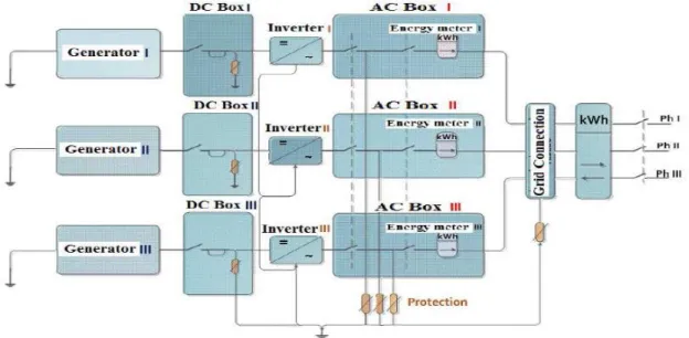
The procedure of fault detection in grid connected PV systems based on the current and voltage indicators described in this review was tested in a grid connected PV system located in the Centre de Développement des Energies Renouvelables (CDER), Algeria. This PV system of 9.6 kWp is divided in three sub-arrays of 3.2 kWp each one, which are connected to 2.5 kW (IG30 Fronius) single phase inverters. Each sub-array is formed by 30 PV modules (Isofoton 106W-12V) in a configuration of two parallel strings, Np=2, of 15 PV modules in series, Ns=15.

Fig. 2.1- General Scheme of the PV system installed in CDER

This PV system includes a monitoring system using an Agilent 34970A for the data acquisition as well as two pyranometers (Kipp & Zonen CM 11 type) and a reference solar cell to measure irradiance at different planes. One of the pyranometers and the reference cell are installed at two different places of the PV plant to measure irradiance in the tilted plane. A second pyranometer measures the irradiance in the horizontal plane. On our work in this thesis we use the measurement from the second pyranometer correspondent to the horizontal irradiance. For the measurement of the temperatures the monitoring system includes k type thermocouples.

2.3.2 PV module Parameters extraction

In order to find the main five parameters of the PV module, Isofoton 106/12, the well know “Five parameter” model was used. In this method, the relationship between output current and voltage is given by the following nonlinear implicit equation:

𝐼 = 𝐼𝑃𝐻− 𝐼0[exp (𝑉+𝑅_𝑛𝑉𝑆𝐼

𝑡 ) − 1] − (

𝑉+𝑅𝑠.𝐼

𝑅𝑠ℎ ) (2.1)

Where the five parameters are: cell photocurrent (IPH); diode reverse saturation current (I0); ideality

factor (n); series resistance (Rs) and shunt resistance (Rsh). I and V are the output PV cell current and

voltage, Vt is the thermal voltage. The effect of temperature in output voltage and current are also

incorporated into the model. A nonlinear regression algorithm has been applied to both data sets; measured I-V data from the PV system and data generated by the previous model, in order to minimize the following quadratic function [37-39]:

𝑆(𝜃) = ∑𝑁 [𝐼_𝑖

𝑖=1 −𝐼(𝑉𝑖, 𝜃)]2 (2.2)

where: 𝜃 = (𝐼𝑃𝐻, 𝐼0, 𝑛, 𝑅𝑠,𝑅𝑠ℎ)

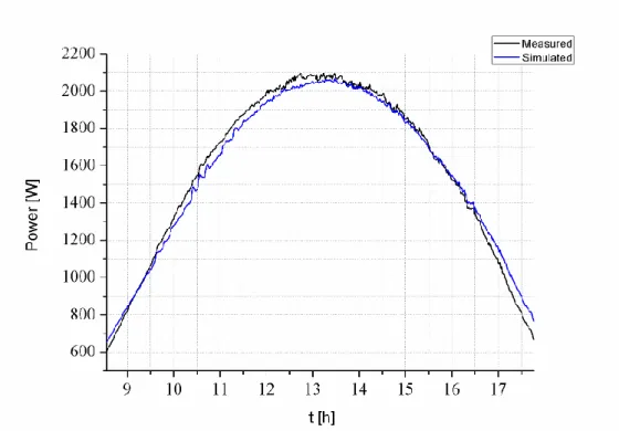
This model has been tested using the operational data from the grid connected branch of 3.2 kWp of the CDER PV system. For the simulation of the branch, the environmental conditions of irradiance and cell temperature had to be linked to the simulation model. Figure 2.3 compares the measured and simulated power at DC side, of this branch (Array of the main PV system) with the real data between 8:33 and 17:47 of that day.

As can be seen, there is a good agreement between simulation results and monitored data for the time evolution of the main PV system parameters.

2.3.3 Fault Diagnosis based on energy yields, current and voltage indicators

This approach is based mainly on the observation of the measured performance ratio (PR). Although this parameter gives a global idea of the system behavior, its practical use for the identification of malfunctioning components is limited. The PR for a particular system during certain period is not suitable quantity to indicate in which way the PV system can be improved due to the following reasons:

 Performance ratio gives no intuition in different component losses;

 There is no way to identify improperly functioning components;

 The numerical simulation must be based on reliable simulation tools and models validated experimentally.

2.3.4 Power loss factors in PV systems

2.3.4.1

Quantifying power losses

International Energy Agency (IEA) Photovoltaic Power System Program established four performance parameters that define the overall system performance with respect to the energy production, solar resources, rated power and overall effect of system losses. These performance parameters are the reference yield (Yr), array yield (Ya), final yield (Yf) and the performance ratio (PR) which is defined

as a ratio of the measured system efficiency and the nominal efficiency of the PV modules. A detailed explanation of each one of the parameters will be explained in detail:

 Reference yield (Yr)

The reference yield is the total in-plane irradiance (Hi) divided by the reference irradiance (Gref). It

represents the equivalent amount of hours necessary for the array to receive the reference irradiance. This reference yield defines the solar radiation resource for the PV system. The value of the reference yield (Yr) is calculated in Equation 2.3:

𝑌_𝑟 = 𝐻𝑖

𝐺𝑟𝑒𝑓 (2.3)

where:

Hi= Total in-plane irradiance [Wh/m2]

Gref= reference irradiation at STC (1000 W/m2)

 Array Yield (Ya)

The array yield is the energy generated by the PV array (Wh) divided by the rated output power of the PV array (Wp). It gives the number of hours where the installed PV system produces its rated output DC power. The value of the array yield (Ya) is calculated in Equation 2.4:

𝑌_𝑎 = 𝐸𝑑𝑐

𝑃𝑟𝑒𝑓 (2.4)

where:

Edc= energy generated by the PV array [Wh]

Pref= maximum power output of the PV array [Wp]

Ya [Hours]

 Final Yield (Yf)

The final yield is the AC energy output (consumed energy) divided by the rated DC power (Pref) of the

installed PV array. It represents the number of hours that the PV array operates at its rated power to produce that amount of AC energy. The value of the final yield (Yf) is calculated by Equation 2.5:

𝑌𝑓 =_𝑃𝐸𝑎𝑐

𝑟𝑒𝑓 (2.5)

where:

Eac= consumed PV energy [Wh]

Pref= System rated power [Wp]

Yf [Hours]

 Performance Ratio (PR)

The performance ratio (PR) quantifies the overall effect of losses on the rated DC output due to inverter efficiency, wiring mismatch and other losses when converting from DC to AC power; PV module temperature; incomplete use of irradiance by reflection from the module front surface; soiling or snow; system down-time; and component failures [2]. The value of the performance ratio (PR) is calculated by Equation 2.6:

𝑃𝑅 =𝑌𝑓

𝑌𝐴 (2.6)

Therefore, the performance ratio gives a global idea of the system behavior and the overall system performance but it is not a good indicator for the identification of improperly functions of the PV system.

2.3.4.2

Power loss factors

This topic was already described in more detail in a previous section but in order to better understand this review, here is a quick overview of the loss factors in a PV system. Overall losses in PV systems happen in both DC and AC sides and are influenced by a number of factors. Figure 2.4 shows the main factors of power losses in PV systems:

Fig. 2.4- Loss mechanisms in PV systems

The main loss factors are the following [40]:

 Capture losses

This kind of losses occur mainly at the DC side of the PV system and they are attributed to operating temperature, PV efficiency temperature dependency, dependency on solar irradiance level, shading and losses when sunlight is at a high angle of incidence (AOI).

 System Losses

They are mainly referred to the power conditioning units, which in our case are the DC-DC converter (MPPT) responsible to extract the maximum available power from the PV plant and the DC-AC converter. These two parts are usually presented by their efficiencies due to the ohmic power losses in the static switches forming part of both converters. In this previous work, the investigation was focused on the losses and malfunctions at DC side because until then and now there is no common way to prevent excessive losses or components breakdown at this part of the PV system contrary to the AC side where the inverters are well protected against improperly functions.

2.3.4.3

The capture losses – AC side

The capture losses can be divided into two kinds of losses [41]:

 Thermal capture losses (Lct)

The crystalline PV modules have a temperature coefficient for the maximum power point of -0.0044/°K. Also, the module efficiency at standard test conditions (STC) is defined at 25°C. Depending on the wind speed and the type of mounting of the PV modules, free-standing or roof integrated, there is a temperature rise of the modules with respect to the ambient of 20°C to 40°C at 1000 W/m2_{. The corrected temperature at real working irradiance and a standard temperature of 25°C}

can be obtained by the simulation model where the input are the monitored irradiance and a fixed temperature of 25°C. The normalized capture losses can be determined by the following Equation:

𝐿𝑐𝑡_𝑠𝑖𝑚 = 𝑌𝑎_𝑠𝑖𝑚(𝐺, 25º𝐶) − 𝑌𝑎𝑠𝑖𝑚(𝐺, 𝑇𝑐) (2.7)

where:

Lctsim are the simulated thermal losses, Yasim(G,25°C) is the normalized energy yield at real working

irradiance and 25°C of temperature, and Yasim(G,Tc) is the array yield at real working irradiance and

real module temperature, Tc. Normalized thermal losses can give us the amount of power losses due the rise of temperature above 25°C. For temperatures below 25°C the Lctsim will be negative

representing a gain on the final performance of the system.

 Miscellaneous capture losses (Lcm)

In this kind of losses we gather all the other losses such as wiring, low irradiance, dirt accumulation, MPPT errors, and losses caused by faulty operation at the DC side such as faulty strings, faulty modules, partial shadowing, short circuit of modules, etc.

In this previous work the inputs of the simulations of the PV plant were the effective irradiance and the module temperature. Therefore, the simulated capture losses can be calculated with the following Equation:

𝐿𝑐_𝑠𝑖𝑚= 𝑌𝑟(𝐺, 𝑇𝑐) − 𝑌𝑎_𝑠𝑖𝑚(𝐺, 𝑇𝑐) (2.8)

where Lcsim are the capture losses and Yr(G,Tc) is the measured reference yield. Then the simulated

reference miscellaneous capture losses are given by:

𝐿𝑐𝑚𝑠𝑖𝑚 = 𝐿𝑐𝑠𝑖𝑚− 𝐿𝑐𝑡𝑠𝑖𝑚 (2.9)

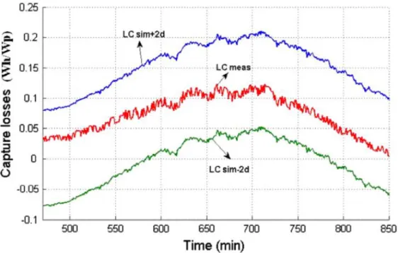
A daily comparison between measured capture losses and simulated capture losses was performed by the system diagnosis and failure detection procedure. The main idea of this method of system diagnosis and fault detection on the DC side of a PV system was based on the continuous check of the measured capture losses. For this purpose, were established theoretical boundaries in which the measured capture losses do not exceed any of them, otherwise the system is considered in faulty operation. The upper and lower boundaries of the inherent capture losses are evaluated by the

introduction of clear sky in-plane irradiance data to the simulation model [42]. Thus, the upper and lower boundaries are calculated by means of statistical approach and in case of PV system under normal operation. The measured capture losses remain the theoretical boundaries as given by the following equation:

𝐿𝑐_𝑠𝑖𝑚− 2𝛿 < 𝐿𝑐_𝑚𝑒𝑠< 𝐿𝑐_𝑠𝑖𝑚+ 2𝛿 (2.10)

where 𝛿 is the standard deviation, calculated in daily basis of simulated capture losses given in case of clear sky conditions.

An example of how these boundaries work is presented on the following figures:

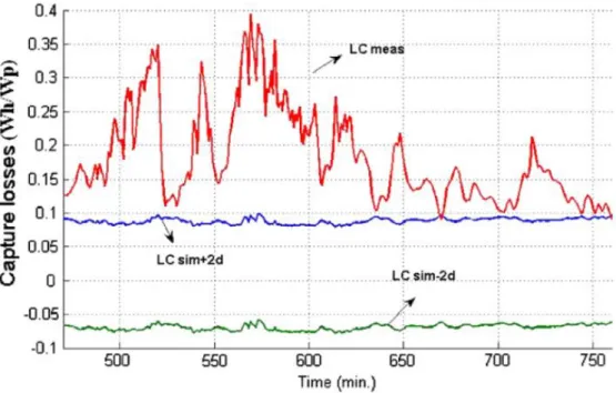
Fig. 2.6- Capture losses evolution on faulty string operation of the PV system

These capture losses indicators at AC side, were used in this previous work in order to simulate and predict capture losses based on the energy yields [2]. With the simulations of the capture losses indicators based on energy yields it was possible to define and predict the system performance with respect to the energy production, solar resources, rated power and overall effect of system losses. In order to know the effect of the system losses on the PV system we compared the DC output power measured in real time with the simulated DC output power.

2.3.5 Indicators for failure detection

The diagnosis procedure described above allows determining whether the actual capture losses are inside or outside the predetermined boundaries. In order to isolate the improperly function detected and determining the failure type, were defined two indicators of the deviation of the DC variables respect to the simulated ones. These indicators are the current and voltage ratios given by the following expressions [2]: meas PV sim PV I I Rc _ _  (2.11) meas PV sim PV V V Rv _ _  (2.12)

where IPV_meas and VPV_meas are the current and voltage measured at the DC output of the PV array

respectively, and IPV_sim , VPV_sim are the results obtained for those parameters in the simulation of the

PV system behaviour by using real irradiance and temperature monitored profiles.

Analysing the ratios, the most probable failure or malfunction is found following the flowchart at Figure 2.7 bellow: