CURRENT RELATION BETWEEN ECOLOGICAL
FOOTPRINT AND COUNTRY RISK PREMIUM
Landry BOUTIN
Dissertation submitted as partial requirement for the conferral of
Master in Finance
Supervisor:
Prof. João Francisco do Rosário, ISCTE Business School, Departamento de Finanças
C
U
R
R
E
N
T
R
E
L
A
T
IO
N
B
E
T
W
E
E
N
E
C
O
L
O
G
IC
A
L
FO
O
T
PR
IN
T
A
N
D
C
O
U
N
T
R
Y
R
ISK
PR
E
M
IU
M
L
an
d
ry Bou
ti
n
In a context of yearly ecological overshoot, policies and financial initiatives for a sustainable management of natural resources appear in increasing number.
This dissertation aims to illustrate the current trends of foreign investments with regard for nature conservation by examining the potential relation between ecological footprint per capita (from the Global Footprint Network database) and country risk premium (as published yearly by Aswath Damodaran).
The analysis is conducted on a panel of 91 countries (43 developed countries and 48 emerging countries) across 17 years (from 2000 to 2016), using panel data analysis methods such as pooled regression, fixed effect and random effect models.
The findings show a significant correlation between the variables, with more intensity for developed countries. The best goodness-of-fit is found using a “random” model for times effects, with the inverse of ecological footprint values as explanatory variables. Therefore the results suggest that the relation between ecological footprint and country risk premium follows an inverse trend, meaning that countries with a very low ecological footprint tend to have unusually high risk premia, and that risk premia tend to get closer to 0% when the ecological footprint is high. The results can be interpreted as a complementarity relation rather than a cause to effect relation, meaning that increased attractiveness to foreign investors by the mean of low country risk premium currently implies a higher consumption of biocapacity.
JEL : Q56 : Environment and development, Sustainability
G15 : International financial markets
Keywords : Ecological footprint, Country risk premium, Investment, Ecological
Num contexto de superação ecológica anual, a políticas e iniciativas financeiras para uma gestão sustentável dos recursos naturais são cada vez mais numerosas.
Esta dissertação tem como objetivo ilustrar as tendências atuais dos investimentos estrangeiros em relação à conservação da natureza examinando a relação potencial entre a pegada ecológica per capita (dos dados de Global Footprint Network) e o risco por país (publicado anualmente pela Aswath Damodaran).
A análise foi realizada num painel de 91 países (43 países desenvolvidos e 48 emergentes) ao longo de 17 anos (de 2000 a 2016), utilizando métodos de análise de dados em painel, como modelos de regressão combinados, efeito fixo e efeito aleatório.
Os resultados mostram uma correlação significativa entre as variáveis, com maior intensidade para os países desenvolvidos. A melhor qualidade de ajuste é encontrada usando um modelo “aleatório” para os efeitos de tempo, com o inverso dos valores da pegada ecológica como variáveis explicativas. Portanto, os resultados sugerem que a relação entre pegada ecológica e prêmio de risco por país seguem uma tendência inversa, significando que países com uma pegada ecológica muito baixa tendem a ter prêmios de alto risco, e que os prêmios de risco tendem a se aproximar de 0% quando a pegada ecológica é alta. Os resultados podem ser interpretados como uma relação de complementaridade ao invés de uma causa para efetuar a relação, o que significa que o aumento da atratividade para os investidores estrangeiros pela média do baixo prêmio de risco por país implica atualmente um maior consumo de biocapacidade.
JEL : Q56 : Meio ambiente e desenvolvimento, Sustentabilidade
G15 : Mercados financeiros internacionais
Palavras-chave : Pegada ecológica, Risco por país, Investimento, Sustentabilidade
Abstract ... I Resumo ... II List of Figures ... IV List of tables ... V List of abbreviations ... VI 1 Introduction ... 1 2 Literature review ... 2
2.1 Natural capital and ecological context ... 2
2.2 A growing concern for nature preservation ... 3
2.3 Natural capital investment and economic benefits... 6
2.4 Environmental performance and country risk premium ... 7
3 Theory and hypotheses ... 11
4 Data and Sources ... 13
4.1 Country risk premium ... 13
4.2 Ecological footprint ... 13
5 Methodology ... 15
6 Results. ... 17
6.1 Presentation and analysis of the results... 17
6.1.1 Dataset with the entire list of countries ... 17
6.1.2 Results when using 1/EF as the explanatory variable ... 25
6.1.3 Comparison between emerging and developed countries ... 28
6.1.4 Verification of the hypotheses ... 33
6.2 Interpretation of the results ... 34
7 Conclusion ... 37
8 Bibliography ... 38
9 Appendices ... 42
9.1 Appendix 1 : List of countries of the data set ... 42
9.2 Appendix 2 : Descriptive statistics for all countries... 44
9.3 Appendix 3 : Descriptive statistics for emerging countries ... 44
9.4 Appendix 4 : Descriptive statistics for developed countries ... 44
Figure 1 : Mean and standard deviation of country risk premium by country. Figure 2 : Observations of country risk premium and ecological footprint.
Figure 3 : Observations a trendlines of country risk premium (y axis) and ecological footprint (x axis) per year.
Figure 4 : Shapiro test on CRP for all countries. Figure 5 : Shapiro test on EF for all countries.
Figure 6 : Kendall’s correlation test between EF and CRP for all countries. Figure 7 : Spearman’s correlation test between EF and CRP for all countries. Figure 8 : Pooling OLS model results for all countries.
Figure 9 : “Within” time effect model results for all countries. Figure 10 : F-test for time effects results for all countries. Figure 11 : “Random” time effect model results for all countries. Figure 12 : Breusch-Pagan test for random time effects for all countries. Figure 13 : Hausman test for all countries.
Figure 14 : Kendall’s correlation test for CRP and 1/EF.
Figure 15 : Pooled OLS regression summary between CRP and 1/EF. Figure 16 : “Random” time effect model summary between CRP and 1/EF. Figure 17 : Breusch-Pagan test for time effects for CRP and 1/EF.
Figure 18 : Hausman test for CRP and 1/EF.
Figure 19 : Observations of EF and CRP per year and representation of the “random” model using 1/EF . Figure 20 : Pooled OLS regression summary for emerging countries.
Figure 21 : “Random” model with time effect for emerging countries. Figure 22 : Breusch-Pagan test for time effects for emerging countries Figure 23 : Hausman test for emerging countries
Figure 24 : “Random” model with time effect for developed countries. Figure 25 : Breusch-Pagan test for time effect for developed countries. Figure 26 : Hausman test for developed countries.
Table 1 : Descriptive statistics of the entire dataset. Table 2 : Random effects per year for all countries.
Table 3 : Random effects per year for all countries using 1/EF. Table 4 : Descriptive statistics of the emerging countries dataset. Table 5 : Descriptive statistics of the developed countries dataset. Table 6 : Random effects per year for emerging countries using 1/EF. Table 7 : Random effects per year for developed countries.
CDS : Credit Default Swap CRP : Country Risk Premium EF : Ecological Footprint
EFc : Ecological Footprint of consumption EFp : Ecological Footprint of production Eft : Ecological Footprint of trade
ERISC : Environmental Risk Integration in Sovereign Credit analysis EU : European Union
GDP : Gross Domestic Product Gha : global hectare
GWP : Gross World Product Ha : hectare
HDI : Human Development Index IFC : International Finance Corporation
IHDP : International Human Dimension Programme IMF : International Monetary Fund
IUCN : International Union for Conservation of Nature IWI : Inclusive Wealth Index
MSA : Mean Species Abundance OLS : Ordinary Least Squares UN : United nations
UNEP : United Nations Environment Programme UNU : United Nations University
US$ : United States Dollar USA : United States of America
1 Introduction
The 21st century has come with growing concerns for ecological sustainability. The
constant seek for economic growth has led to over-exploiting natural resources (Wackernagel et al., 2002), and today, all of the developed countries produce, consume and trade beyond nature’s regenerative capacity. All industries share a part of responsibility and a part of consequent risk, and the financial sector is not an exception. It even is an critical sector in the way it is related to all others, giving access to capital, investments, debt and insurances, showing the path and leading the way of the global economy.
This dissertation aims to identify the current trend in international finance regarding ecological sustainability by examining the relation between ecological footprint per capita and country risk premium. Ecological footprint is a measure of consumption of natural resources created by the Global Footprint Network (Borucke et al., 2013). Country risk premium measures is computed with sovereign credit ratings and measures the risk associated to investments in a specific country (Damodaran, 2013). The link between these two factors would somehow illustrate the current link between sustainability and economic growth, natural capital preservation and financial profitability.
After providing a review of the literature concerning the current ecological context and the previous findings regarding country risk premium and environmental performance, this dissertation will display a statistical panel data analysis to examine the existence, intensity and nature of the relation between ecological footprint and country risk premium.
2 Literature review
2.1 Natural capital and ecological context
“Natural capital is the spectrum of physical assets within the natural environment that
deliver economic value through ecosystem services” (Voora and Venema, 2008). The
benefits flowing from natural capital can be benefits to society (e.g. mangroves preventing floods, plants photosynthesis providing oxygen) or benefits to economy (e.g. raw materials, energy, pollination, biodiversity). Natural capital is made of renewable and non-renewable resources. Renewable resources are generated continuously, which is called Earth’s regenerative capacity, and while some of these resources are destroyed or transformed every year (fruits rotting, animals dying,…), some of it remains and increases the natural capital stock. Our economy cannot be sustainable if we draw on natural capital beyond its regenerative capacity, as it means taking from the natural capital stock and entirely depleting it at some point. Facing this reality, Wackernagel et al. (2002) figured that the only way to prevent this was to have knowledge of how much of the total biocapacity Humanity was using. By comparing estimates of the yearly biocapacity and human use of natural resources, they found that the consumption had begun exceeding the biocapacity in the early 1980s. They called this phenomenon the ecological overshoot of human economy.
In a similar perspective, the first estimation of the world’s natural capital in monetary value was made in 1997. It was valued at 33 trillion 1995US$ per year (Costanza et al., 1997), the equivalent in US$ of 2019 is 55 trillion US$. The same team of researchers updated their work in 2014 (Costanza et al., 2014) with more accurate estimates both for the value of the different kinds of ecosystems in US$/year/ha (de Groot et al., 2012) and for the total area of each ecosystem, taking into account the degradation of natural capital between the two studies. The new natural capital valuation was made at 125 trillion 2007US$ of per year (154 trillion US$ per year in 2019), with a total degradation estimated to 24.5 trillion US$ per year between 1997 and 2014. As a tool for comparison, the GWP (Gross World Product) was estimated at 84.74 trillion US$ in 2018 according to the IMF1.
As explained by Aronson et al. (2006), natural capital constitutes a limiting factor of economic growth, and as indicated previously, humanity is not only ignoring it but
degrading it, thus enhancing its limiting effect and ironically dooming economic growth for the sake of economic growth. In addition to this, the foreseen growth of global population (United Nations Department of Economic and Social Affairs, 2017) and demand for energy and food (Valin et al., 2014) in the coming decades call for an increased need and therefore an increased use of natural resources. If the trend is not reversed, this path will ultimately lead to an ecological and economic crisis (Steffen et
al., 2018; Laybourn-Langton et al., 2019).
2.2 A growing concern for nature preservation
Although the world remains on the path of overconsumption and ecological crisis, it is noticeable that there has been a rising concern and awareness about natural resources management and nature conservation in the beginning of this century. There is a considerable amount of initiatives in favour of the environment that have been created in the last 30 years.
• The Equator Principles : A set of 10 principles constituting a risk management framework for assessing and managing environmental and social risks (The Equator Principles, 2013). The framework is officially adopted by 96 financial institutions in 37 countries.
• The UN Principles for Responsible Investment : A set of 6 principles to lead investors and asset managers to incorporating ESG factors in their financial decisions(Principles for Responsible Investment, 2019).
• The IFC Performance Standards : A set of standards created in 2012 that the clients of the International Finance Corporation have to apply2.
• The Banking Environment Initiative : An initiative created in 2010 and convened by the University of Cambridge Institute for Sustainability Leadership to lead the banking industry into directing capital towards environmentally and socially sustainable economic development3.
• The UNEP Finance Initiative : a partnership between United Nations and financing sector created in 1992 to promote sustainable finance. More than 240
2https://www.ifc.org/wps/wcm/connect/Topics_Ext_Content/IFC_External_Corporate_Site/Sustainability -At-IFC/Policies-Standards/Performance-Standards
financial institutions works with the United Nations Environment Programme for this initiative4.
• The Dutch Association of Investors for Sustainable Development (VBDO) : An association of financial institutions created in 1995 in Netherlands aiming to create a sustainable capital market5.
• The Natural Capital Finance Alliance : An association providing tools and methods for financial institutions to manage the risks of their environmental impacts and dependencies6
All of these initiatives appearing at the end of the 20th century and the beginning of the
21st show that there is a will from the financial sector to orientate their industry towards
environmental sustainability.
As mentioned earlier, environmental performance is not always linked to financial performance, but studies have shown that carbon emissions can lead to lower financial performance (Ganda and Milondzo, 2018). Whether or not one leads to the other, it has also been shown that some investors are taking companies from high carbon emitting industries out of their portfolio and that even if companies are not directly impacted on capital markets, “carbo intensive” industries are underperforming (Sebag, 2018).
This recent emphasis of ecology has also lead to growing need for research and data on this topic. A good example of environment related data collection is the work of the Global Footprint Network, who have kept up on Wackernagel’s work in estimating the consumption and production of the world’s countries. They’ve developed a methodology to measure a country’s ecological footprint and biocapacity (Borucke et al., 2013) in a bid to assess their sustainability. There is similar to Wackernagel’s in the way that they convert everything in the same unit (global hectare) in order to be able to compare the countries between them. The ecological footprint of a country is the sum of the ecological footprint of its consumption and the one of its trade balance. The biocapacity is the total natural resource production capacity of the country. They also get similar results, although a bit more alarming as they indicate that Earth’s overshoot day (the day of the year at which on year of regenerative capacity has been used) is earlier than the 31st of
December since 19707. 4 https://www.unepfi.org/about/ 5 https://www.vbdo.nl/en/ 6 https://naturalcapital.finance/about-ncfa/ 7 https://www.overshootday.org/newsroom/past-earth-overshoot-days/
Another organisation, CDP, assesses the environmental performance of cities and companies since 2003. Their database for companies is one of the largest and is the result of yearly surveys about carbon emissions, water use, forest use and the different related policies or decisions made by the companies. The rise of awareness also reaches financial institutions who are starting to take environmental performance into consideration for investments, insurances or loans. The CDP database has been used in 2018 by Euronext to create a new index called “Euronext CDP Environment Finance” and nicknamed “the green CAC 40” made of the 40 firms with the highest CDP rankings among the SBF 120. A similar index already exists in the USA, the Global Climate Change Leaders index from STOXX, which outperformed the STOXX Global 1800 in 2018 (Fay, 2018). Other environmental initiatives have been launched by financial institutions. Sycomore Asset Management has created the NEC (Net Environmental Contribution) in partnership with BNP Paribas (Péladan, 2018). It is a tool based on a specific industry’s environmental impact to compare products and companies against their competitors on a scale from -100% to +-100% (Most negative to most positive contribution). A good example for initiatives in more specific fields is CDC (Caisse des Dépôts et Consignations). The bank has used the help of GLOBIO and their MSA (Mean Species Abundance) square meter measure to create a method to assess a company’s impact on biodiversity (CDC Biodiversité, 2017).
This relatively new practice of measuring environmental performance for companies and countries in every possible way as lead to the identification of new links of responsibility and impact. Globalisation an international trade can now make countries responsible for a fair part of another country’s ecological impact, even if located on the other side of the globe. Steen-Olsen et al. (2012) have studied the several aspects of the ecological footprint of European Union citizens. They have found that EU citizens’ carbon footprint is twice higher than the world’s average, 31% of which happens outside of the EU and is due to European demand and consumption. They also indicate the same results for land use. Another study from Lenzen et al. (2012) has estimated countries’ impact on species around the world by linking more than 7000 threatened species from the IUCN red list to more than 15000 commodities from 187 countries and analysing the flows of these commodities. The results show that developed countries (mainly United States, countries from the EU and Japan) tend to be net importers of such commodities, threatening species in developing countries that are exporters. The reason for these trades can either be the lack of exotic products in demanding countries (no coffee or cocoa production in
European countries), or species protection policies implemented in developed countries preventing them from having a production that could be harmful to local species, leading them to buy the commodities from countries where such policies don’t exist. Their study also shows that the two main factors of threats to species related to international trade are agriculture (139 species are threatened by palm oil, rubber or cocoa production in Malaysia) or trade related pollution (304 species threatened by pollution in China). This study has lead the same authors to create world maps showing the number of species threatened by one country in different areas (Moran and Kanemoto, 2017). The results show for example that USA’s consumption mainly impacts species in central America, western Europe and southern Asia, where Europe’s consumption mainly affects Asia, especially western, and Africa.
2.3 Natural capital investment and economic benefits
The exact reasons why ecological damage is not yet slowing down as a result of growing awareness are not easy to understand. The first reason coming to mind is financial performance and opinions on its relation with environmental performance in a company vary depending on the industry and context (Molina-Azorín et al., 2009; Muhammad et
al., 2015; Nor et al., 2016; Di Pillo et al., 2017; Alexopoulos et al., 2018). However,
several studies have shown that investments in natural capital conservation and/or restoration is beneficial. The failure to protect biodiversity was estimated at 140 billion US$/year, while developing a global network of nature resources to prevent the loss would cost 45 billion US$ (Balmford et al., 2002). Another study estimates the potential loss at 14 trillion US$/year by 2050 (Braat et al., 2008). Sumaila et al. (2017) have shown how reaching Aichi biodiversity targets by 2020 (agreed upon by the 193 countries of the Convention on Biological Diversity) would be economically beneficial. They estimate that reaching the goal and reversing biodiversity loss in the entire world by 2020 would require investments from 150 to 440 billion US$, which represents 0.002 to 0.007% of the Gross World Product. They take as an example the case of fisheries. The world’s fisheries account for 16% of the global protein intake and suffer a 50 billion US$ yearly loss due to unsustainable fishing. They estimates that the removal of harming fisheries would cost 20 billion US$ and generate yearly returns of 124.8 US$. They also indicate that halving the deforestation rate by 2030 would avoid 3.7 trillion US$ of climate change related damage. Another study regarding potential climate change related damage was
conducted in 2015 (The Economist Intelligence Unit, 2015). The researchers used the DICE model (a model of the global economy including climate change made by William Nordhaus) to compute the climate change value-at-risk, they have estimated several Values-at-risk both on a private and governmental point of view, and for several increases of temperature between now and year 2100. The values range from 4.2 to 43 trillion US$ of potential loss. Studies have also shown that direct investment in natural capital restoration projects yield positive returns in the long term, with varying risks and potential returns based on the nature of the ecosystem restored (de Groot et al., 2013; Blignaut et
al., 2014).
2.4 Environmental performance and country risk premium
The most extensive researches about the links between economy, finance and ecology around the world are made by the United Nations Environment Programme. Their main goal is to include environmental factors in usual economic and financial indicators. They have started by creating a wealth measure that includes ecological development to assess a country’s sustainability (UNU-IHDP and UNEP, 2012). It is called the IWI (Inclusive Wealth Index) and is computed using countries’ natural, manufactured, human and social capital. It is intended as a replacement of GDP (Gross Domestic Product) and HDI (Human Development Index). They show that countries’ growth rates are very different if IWI is used rather than GDP, mainly because it uses a stock metric (capital) instead of flows, which according to UNEP is more representative. This way, the average growth rate per annum of Nigeria during the two decades preceding 2012 could vary from +2.5% (GDP) to -1.8% (IWI).
The UN Environmental programme has also conducted researches on the impact of natural resources use on sovereign debt rating. Sovereign credit rating is an independent assessment of the creditworthiness of a country or sovereign entity8. The main institutions
delivering these ratings are Moody’s and Standard & Poor’s. UNEP’s reports about sovereign debt are called ERISC (Environmental Risk Integration in Sovereign Credit Analysis). In the first one (UNEP, 2012) they study the cases of five countries with different rankings from AA+ to BB (ratings from S&P) and analyse their exposure to natural resources related risks (effects of commodities price volatility and variation of the
biocapacity on GDP). Their results lead them to the conclusion that countries have a certain level of climate risk resilience which can be measured using economic indicators and make them less exposed to potential losses due to environmental changes. They suggest as a conclusion that climate risk resilience could be used in sovereign credit rating. This report lead Moody’s to adapt their methodology and explain how climate change was accounted for in their ratings (Moody’s, 2016). They explain that climate risk is not directly valued but is taken into account in the way it affects economic strength, institutional strength, fiscal strength and mostly susceptibility to event risk. Their parameter called susceptibility is the main tool for climate risk assessment as it is a function of two components. It is made at about 70% of the country’s exposure to climate change risks which is determined using the geographic location and area as well as the economic diversification (if a country’s entire economy relies on the production of one specific commodity, the country is extremely sensitive to any event affecting this production). The second component is resilience, as suggested in the ERISC report. Resilience is assessed using a country’s development level: its wealth, fiscal flexibility, debt level, environmental policies, insurance or saving funds for natural disasters,… Anything that constitutes a resource for adaptation to particular ecological events is taken into account for the resilience. The degree to which a country is exposed to climate change risk and the degree to which it is able to adapt to ecological changes both constitute its susceptibility. Moody’s found that when separated, susceptibility had a strong correlation with creditworthiness rating. Susceptible countries tend to be developing countries that are often net exporters of natural resources and therefore more exposed and sensitive to climate shocks. S&P has also communicated about the climate change factor in their ratings (S&P Global Ratings, 2015). They assessed the way climate change increases natural catastrophes related risk, the estimate the increase at 20%. They also indicated that variations in credit ratings due to climate change were negligible for developed countries but more important for emerging countries, and that catastrophe insurance (also cited by Moody’s for resilience) could lower the climate change risk.
The latest ERISC report showed a particular focus on food prices volatility (UNEP, 2016). They argue that the growing population and demand for food will increase the gap between food supply and demand along with variability in food production and therefore increase the volatility of food prices, which is why it is important to assess the sensitivity of countries to food prices volatility. Their main method is to submit the countries to a stress test of food price shock, simulating a sudden doubling of food prices and to analyse
the effects it would have on countries. The results show that such an event would negatively affect the GDP of 101 out of the 110 countries analysed, and the current account of 69 of them. The rarer cases of positive effects happen for net food exporters, but it is not representative as it is the case of a price increase: a similar price shock with prices suddenly decreasing would have a negative impact on net exporters, which also makes them sensitive. It is more relevant to look at the level of impact among the countries. The results also show that high sovereign credit ratings correlate with low vulnerability to food prices volatility. When comparing these results with the ecological footprint of the countries in 2005, they remark that countries with high ecological footprints (and therefore high responsibility in climate change and environment issues) are the less vulnerable to food price shocks. An interesting aspect of the report is that the researchers revaluated the sovereign credit ratings of 78 countries taking into account the vulnerability to food prices volatility. They found that 58 out of the 78 countries would be downgraded.
Obviously, sovereign credit ratings are used by investors to know the risk of governmental bonds in every country of the world, but they are also used in other types of investment like equity investment to compute the risk related to a specific foreign country. As explained by Arouri et al. (2012) and (Horn et al., 2017), even if the standard CAPM formula is often used to estimate the cost of equity, it is not enough for emerging markets as they bring additional risks. It is a growing matter because developing countries are becoming more important in the global economy while conserving higher risks and required returns (Bekaert and Harvey, 2014). The share of GDP of emerging countries in the world keeps increasing but the total market capitalisation doesn’t grow accordingly, which is how the authors justify that even in a globalisation context it still makes sense to differentiate developed countries and emerging countries for investments. In addition to this, Ernst and Gleißner (2012) find that using a premium while computing cost of equity tends to make estimations closer to reality.
While the utility of the country risk premium is justified, its computation remains controversial. Aswath Damodaran is one of the most cited references in terms of market risk premium, especially for country risk premium (Fernàndez et al., 2011). The first one consists in using the CDS (Credit Default Swap) yield spread between the concerned country and the one of the USA (which is considered without default risk), this method is simple and effective but is limited to countries with a CDS yield and sometimes results in a negative risk premium when the country’s CDS yield is lower than USA’s, which is
counterintuitive. The second method consists in computing the average CDS spread between countries and USA for each credit rating class and using the results to determine the risk premium for each country with its credit rating (Damodaran, 2013). This is how he is able to yearly make available a list of country risk premia (CRP) for all the countries with sovereign credit ratings9. The CRP can then be used to add country risk to cost of
equity. Although there are alternatives and critics to Damodaran’s method, it is very often used and shown to be relatively close to the mean cost of equity estimates computed by the different methods (Horn et al., 2017). When investing abroad, it is now very common for investors to take country risk into account. The studies of Busse and Hefeker (2005) and Hayakawa et al. (2011) respectively based on panels of 93 countries over 22 years and 83 countries over 19 years both show that country risks have a negative impact on foreign direct investments inflow, which is doubled for emerging countries.
3 Theory and hypotheses
The research conducted by UNEP (2012 and 2016) indicates a link between environmental impact and sovereign credit ratings, either in the degree to which countries are vulnerable to climate risks or in their own impact on natural capital. As country risk premia are often computed with the help of sovereign credit ratings, it is possible to suggest that a country’s risk premium (and therefore its attractiveness to investors) is somehow related to its impact (positive or negative) on natural resources. In order to compare countries between them in an ecological dimension, the best tool is the Global Footprint Network’s ecological footprint per capita. It allows comparison without scale issues.
It would not be relevant to expect a model that fully explains the variance of country risk premia with only one variable (ecological footprint). It goes without saying that explaining country risk premium requires multiple explanatory variables. Rather than fully explaining a country risk premium, the goal of this dissertation is to identify a potential relationship between ecological footprint and country risk premium, which will be examined using several hypotheses.
H1 : There is a significant correlation between the ecological footprint and the risk premium.
Ha : There is no significant correlation.
This first hypothesis is the beginning of the analysis, the presence of a correlation between these variables would induce the possibility of relating them in a model. A positive correlation would mean that countries with a high consumption of natural resources tend to have a higher risk premium and therefore to be considered riskier. On the contrary, a negative relationship would indicate that investments are safer in countries with a high ecological footprint. The absence of significant correlation would mean that country risk is not associated in any case with environmental performance. The validation of this first hypothesis is suggested by the work of the UNEP in their ERISC studies and by the several evidences of investors’ growing interest for environmental performance.
H2 : The relationship between ecological footprint and country risk premium varies across time.
As said earlier, environmental sustainability has gained interest in the financial sector in the last 30 years (Molina-Azorín et al., 2009; Di Pillo et al., 2017; Alexopoulos et al., 2018; Ganda and Milondzo, 2018; Sebag, 2018). The growing concern for ecology may have increased the correlation or affected the relationship in a way, or unobserved factors could lead to different results across the years. The absence of time influence on the slope can either indicate that the relationship has always been the same regardless of the year or that the analysis is not conducted on a long enough time period.
H3 : The relationship between ecological footprint and country risk premium varies across countries.
Ha : The specific country has no influence on the relationship.
This hypothesis is the same kind as the second one, it is possible that some characteristics of a country, as for example susceptibility as used in Moody’s methodology (Moody’s, 2016), affect the relationship. The verification of the alternative hypothesis would suggest that the ecological footprint affects all the countries’ risk premia in the same way.
H4 : The correlation between ecological footprint and country risk premium for emerging countries is different from developed countries.
Ha : The development of the country does not affect the relationship.
This hypothesis is a potential derivation of the third hypothesis, as developed countries tend to have lower risk premiums they could be affected in a different way than emerging countries. The data leading to this hypothesis comes from Hayakawa et al. (2011), who found that country risk affects foreign direct investment inflow to a higher degree for emerging countries than for developed countries.
4 Data and Sources
This study examines the relationship between two variables : ecological footprint and country risk premium. As the goal is to compare countries to obtain a global trend, data from as many countries as possible is needed. For data availability reasons, the selected time period is 2000 to 2016.
4.1 Country risk premium
The data used for country risk premia (CRP) comes from Aswath Damodaran’s website10.
As he uses two different methods to compute the premia (Damodaran, 2013), the sovereign credit rates method (using Moody’s ratings) has been selected because it is computed for more countries (as mentioned earlier the CDS yield method is applicable only on countries with credit default swaps). In his databases, Damodaran offers the possibility to multiply the risk premia by the rate ratio of equity volatility over government bond volatility for each country in order to adjust the CRP to the additional volatility of the equity market. It was not done for this study for two reasons. First, Damodaran only gives the data about the concerned volatilities in the last years’ databases and a lot of countries are missing at least one of the two, there is a big lack of data to compute the ratio for each country and each year. Second, Damodaran sometimes uses an average equity/government bond volatility ratio of 1.5 to adjust the CRP. Doing so in this study would be irrelevant as multiplying all of the values by 1.5 would not change the results. After selecting the countries for which the data was available for all the years (2000-2016), 91 countries remained.
4.2 Ecological footprint
The ecological footprint is a measure of impact on the environment. It was created by the Global Footprint Network. The advantage of this measure is that it represents a common unit to compare anything in the way it affects the environment. The method to measure a country’s ecological footprint of consumption (EFc) starts with measuring the ecological footprint of production (EFp) (Borucke et al., 2013). The EFp is the total bio-productive
area of land necessary to produce all of the primary goods harvested in the country (cropland, grazing land, forestland and fishing grounds), to support the built up area (cities) and to absorb the emitted carbon (forestland again). Once the total necessary area in hectares of each type of land is measured, it is converted to global hectares (gha). A global hectare is an hectare of land with the world’s average productivity. The conversion is made by multiplying the area of each land type by an equivalence factor (how many times does an hectare of this land type produce the production of a gha). Once all of the bio-productive areas are converted into gha they can be added. The sum is the EFp. The same steps are used to measure the necessary area to produce internationally traded goods and absorb the emissions related to their trade. This is how the ecological footprints for import and export are computed, the difference between which gives the ecological footprint of trade (EFt). Adding the EFt and EFp gives the EFc, which is simply called ecological footprint or EF in this paper. The major advantage of this measure is that it allows comparison by measuring all of the productions and emissions with the same unit. In order to avoid scale issues in the analysis, the data that will be used is the EFc per capita. A very large amount of the data measured by the Global Footprint Network is available for free and downloadable on their website11. The data was available for all the
17 years and the 91 countries selected with the CRP data. This results in a balanced panel dataset of 2 variables for 91 countries over 17 years, meaning 3094 values.
Using a triennial country classification data set of emerging countries and least developed countries from the United Nations, our 91 countries were classified in least developed countries, emerging countries and developed countries. 48 of the countries are emerging countries and 43 are developed countries, there are no least developed countries in the dataset and no country in the dataset had its classification changed across the years. Two additional datasets will then be created, one for emerging countries and one for developed countries.
5 Methodology
The analysis of the dataset will start with descriptive statistics (such as mean, median, maximum, minimum or standard deviation) and graphs to evaluate the global trend, what can be expected and eventually plan additional tests.
The first step in the analysis of the relationship between the variables will be a correlation test. The three most frequently used methods for correlation testing are the methods of Pearson, Spearman and Kendall. Pearson’s method is an analysis of the common variance changes between the two variables. Spearman and Kendall compute correlation by ranking the data, Spearman’s formula examines the correlation between values sharing the same rank and Kendall’s formula counts the number of times that two originally associated values end up in the same rank or close to each other. The most commonly used is Pearson’s method but it has been proven to be significant only in the case of normally distributed data (Kowalski, 1972). If the data is not normally distributed, it is preferable to use rank based methods such as Spearman’s and Kendall’s. A Shapiro test and an analysis of the data distribution’s descriptive statistics will therefore be conducted before the correlation test.
The main part of the analysis is a panel analysis. To do so, the “plm” package (Croissant and Millo, 2008) will be used in R (a statistical computing software). The goal will be to find the most efficient model explaining CRP with EF in order to get the best idea possible of the relation between these two variables. The first model to be tested will be a pooled OLS (Ordinary Least Squared) regression which will examine the global linear relation between the two variables with the same intercept and the same slope for every country and every year, in the type of the following equation :
𝑪𝑹𝑷𝒊𝒕 = 𝒂𝟎+ 𝒂𝟏𝑬𝑭𝒊𝒕+ 𝒖𝒊𝒕 (1)
Where a0 is the intercept, a1 is the coefficient, u is the error, i is the country and t is the
year (CRPit and EFit are therefore the CRP and EF for a given country in a given year).
The next step is to look for individual effects from the countries, from time or from both. The individual effects can be fixed effects (variation of the intercept) or random effects (variation in the error).
In order to examine fixed effects (individual variation of the intercept), a “within” model will be used because of the great number of countries (a LSDV model would require creating 91 dummy variables). The following effects will be tested :
• One way country fixed effect :
𝑪𝑹𝑷𝒊𝒕 = 𝒂𝟎𝒊+ 𝒂𝟏𝑬𝑭𝒊𝒕+ 𝒖𝒊𝒕 (2)
• One way time fixed effect :
𝑪𝑹𝑷𝒊𝒕 = 𝒂𝟎𝒕+ 𝒂𝟏𝑬𝑭𝒊𝒕+ 𝒖𝒊𝒕 (3)
• Two ways fixed effect :
𝑪𝑹𝑷𝒊𝒕 = 𝒂𝟎𝒊𝒕+ 𝒂𝟏𝑬𝑭𝒊𝒕+ 𝒖𝒊𝒕 (4)
The random effects, (part of the error that can be associated to the countries or the year without being related to EF) are tested using a “random” model :
• One way country random effect :
𝑪𝑹𝑷𝒊𝒕 = 𝒂𝟎+ 𝒂𝟏𝑬𝑭𝒊𝒕+ 𝑽𝒊 + 𝜺𝒊𝒕 (5)
• One way time random effect :
𝑪𝑹𝑷𝒊𝒕 = 𝒂𝟎+ 𝒂𝟏𝑬𝑭𝒊𝒕+ 𝑽𝒕 + 𝜺𝒊𝒕 (6)
• Two ways random effect :
𝑪𝑹𝑷𝒊𝒕 = 𝒂𝟎+ 𝒂𝟏𝑬𝑭𝒊𝒕+ 𝑽𝒊𝒕 + 𝜺𝒊𝒕 (7)
The significance of the “within” models will be verified with F-tests and the significance of the “”random models will be verified with the Breusch-Pagan test (Breusch and Pagan, 1980). If a “within” or a “random” model is found to be significant, it will be preferred to the OLS model as it takes into account individual effects. A Hausman test will be used to examine the correlation between the random effects and the variables, if the Null hypothesis (no correlation between random effects and variables) is rejected, the fixed effect model will be preferred.
In order to examine the verification of the hypothesis H4, these steps will be repeated for the data set of emerging countries and the data set of developed countries and the results will be compared.
6 Results.
6.1 Presentation and analysis of the results
6.1.1 Dataset with the entire list of countries
The analysis starts by examining the characteristics of the data set.
Variables n Mean sd Median Min Max Range Skew Kurtosis
CRP 1547 0.02 0.02 0.01 0.00 0.18 0.18 1.59 2.53
EF 1547 4.46 2.72 4.03 0.58 17.72 17.14 1.42 3.08
Table 1 : Descriptive statistics of the entire dataset.
The table shows that CRPs range from 0% to 18% (Equator in 2008) with a mean of 2% and a median of 1%, which means that half of the countries in the dataset have a risk premium lower than 1%. The EF range from 0.58 to 17.72 gha/capita (Venezuela in 2016 and Luxembourg in 2003 respectively), with a mean of 4.46 gha/capita close to the median of 4.03 gha/capita. For comparison, in 2016 the world had a biocapacity of 1.63 gha/capita12.
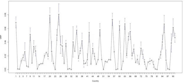
The following graph represents the mean and the standard deviation around the mean of CRP per country. It is intended to illustrate heterogeneity between countries. Each country was associated to a number for the graph’s readability, the correspondence table can be found in appendices13.
Figure 1 : Mean and standard deviation of country risk premium by country.
12 http://data.footprintnetwork.org/#/countryTrends?type=BCpc,EFCpc&cn=5001 13 See Appendix 1 : List of countries of the dataset.
In order to get an idea of the general trend to be expected between the variables, two illustrations will be used. The first one displays the value of the dataset with EF on the horizontal axis and CRP on the vertical axis. The second figure is a set of graphs showing the same relation for each year with a trend line.
Figure 2 : Observations of country risk premium and ecological footprint.
Figure 3 : Observations a trendlines of country risk premium (y axis) and ecological footprint (x axis) per year.
First, these figures suggest a negative trend between the two variables. Countries with a high ecological footprint seem to have a lower risk premium (close or equal to 0%). Based
on the trendlines on Figure 3, it is possible to assume that trend remains the same across the years. Another assumption can be made based on Figure 2 : values of CRP seem to go higher than suggested by the trend for values of EF between 0 and 5, therefore it can be suggested that the relation between the variables may not be linear. The observed data seem to match an inverse relation more than a linear one. To verify this additional hypothesis, another dataset will be created by replacing EF by 1/EF. An additional set of tests will be conducted on the new dataset after the first dataset in order to compare them.
In order to choose between the several correlation tests available, normality tests have been conducted on the variables.
Figure 4 : Shapiro test on CRP for all countries.
Figure 5 : Shapiro test on EF for all countries.
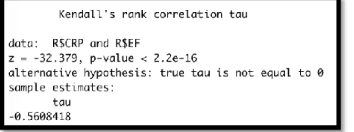
The Null hypothesis of the Shapiro-Wilk normality test is that the distribution of the data matches a normal distribution. The p-value of the test are low enough to reject this hypothesis and conclude that neither the variables are normally distributed. Therefore, the most appropriate correlation tests to be conducted are Kendall’s and Spearman’s.
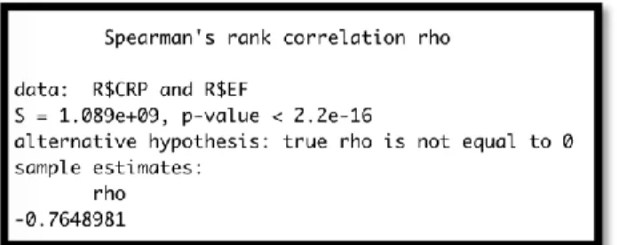
Figure 7 : Spearman’s correlation test between EF and CRP for all countries.
It is important to note that R reported a warning : Spearman’s test excludes the rank “ties”, that is when several values of one of the variables are equal and cannot be ranked. As several developed countries have a CRP of 0%, they are excluded from the test which is why this test is less reliable than Kendall’s. Several conclusions can be made from these tests. First, a significant correlation exists between EF and CRP as the p-value is small enough to reject the Null hypothesis of absence of correlation. Second, the relation is negative according to both tests. Third, the correlation can be said of medium strength with Kendall’s correlation coefficient tau = -0.5608.
Now that evidence for a correlation between EF and CRP have been given, the analysis will aim for finding the nature of this correlation. To do so, several models of panel analysis will be tested. The first model to be tested is a pooled OLS regression.
Figure 8 : Pooling OLS model results for all countries.
Fischer’s test shows that the pooled OLS regression is good, it is significantly different from 0 at the 0.001 level (p-value > 2.22e-16). The result shows that the coefficient for EF has the same degree of significance. Once again it is a negative coefficient and it suggests that a 1% increase of the EF would decrease the CRP by 0.04%. The R squared indicates that the variance of the EF explains 27.88% of the CRP’s variance, which is weak but high enough to validate the hypothesis of correlation.
The purpose of the next tests is to examine the presence of individual effects in the relation between EF and CRP. The first step is to check the presence of fixed effects with a “within” model. After testing the within model with individual effects, time effects and both effects, only the time fixed effect model showed relevant results.
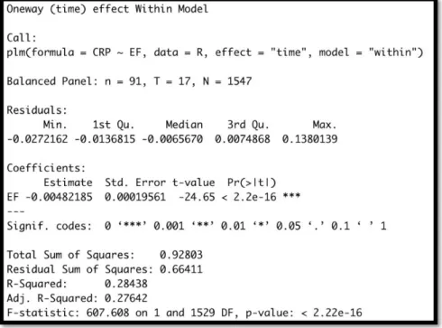
Figure 9 : “Within” time effect model results for all countries.
The model’s summary shows that the time fixed effects are significant to the 0.001 level for each year. The higher R-squared and F-statistic reveal an increased goodness-of-fit in the fixed effect model, meaning the model is better than the pooled OLS. It must however be verified with an F-test for time effects, the result of which confirms the significance of time effects. The conclusion to take from this test is that the observed year has a significant effect on the intercept of the model.
Figure 10 : F-test for time effects results for all countries.
The next step is to look for random effects. As for fixed effects, random effect can be from time, individual (country) or both. After testing all three, the only significant is time effect again, which is consistent with the previous findings.
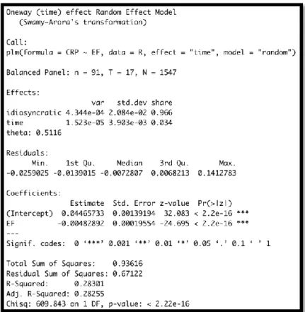
Figure 11 : “Random” time effect model results for all countries.
Again, this regression is significant and even has a slightly improved goodness-of-fit from the fixed effect model. The detail of the effects show that random time effect significantly explain an additional 3.4% of the error. The intercept and coefficient are both significant to the 0.001 degree, the coefficient is still negative. The conclusion that can be made from this is that 3.4% of the residual’s variation can be attributed to the specific year of the observation. The significance for the presence of random time effects can be tested with a Breusch-Pagan test.
Figure 12 : Breusch-Pagan test for random time effects for all countries.
The p-value is low enough to reject the Null hypothesis of absence of significant effects. It means than there is a significant random effect in the panel data and that the random effect model is able to deal better with heterogeneity than the OLS model. After testing seven models, the pooled OLS, “within” fixed time effects and “random” time effects models are significant. As both the “within” and the “random” models show an increase
of goodness-of-fit and take into account the presence of individual effects, both should be preferred to the OLS pooled regression. In order to find the best model between “within” and “random”, a Hausman test can be conducted. The Null hypothesis of this test is that random effects are not correlated to the model’s variables. If the Null is rejected, the fixed effect model should be preferred as the random effects aren’t random. If it isn’t, the best model is the random model.
Figure 13 : Hausman test for all countries.
The p-value of the Hausman test is too high to significantly reject the Null hypothesis, therefore, it holds and indicates that the random effects are not significantly correlated to any of the variables.
In the end, the best model to explain CRP with EF is the random time effects model. It is the model with the best goodness-of-fit. Our final equation for this dataset is the following:
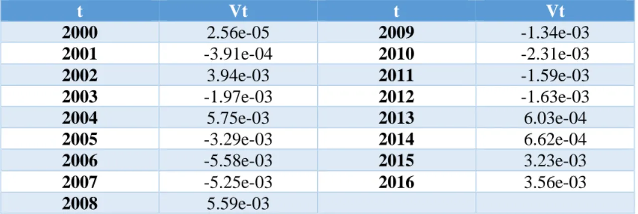
𝑪𝑹𝑷𝒊𝒕 = 𝟎. 𝟎𝟒𝟒𝟕 + (−𝟎. 𝟎𝟎𝟒𝟖 𝑬𝑭𝒊𝒕) + 𝑽𝒕+ 𝜺𝒊𝒕 (8) With Vt being specific to each year :
t Vt t Vt 2000 2.56e-05 2009 -1.34e-03 2001 -3.91e-04 2010 -2.31e-03 2002 3.94e-03 2011 -1.59e-03 2003 -1.97e-03 2012 -1.63e-03 2004 5.75e-03 2013 6.03e-04 2005 -3.29e-03 2014 6.62e-04 2006 -5.58e-03 2015 3.23e-03 2007 -5.25e-03 2016 3.56e-03 2008 5.59e-03
6.1.2 Results when using 1/EF as the explanatory variable
As mentioned at the beginning of the result analysis, the different models have also been tested on the relation between CRP and 1/EF before comparing emerging countries and developed countries.
Not surprisingly, testing 1/EF for normality did not give a different result than for EF, which is why Kendall’s correlation test was chosen.
Figure 14 : Kendall’s correlation test for CRP and 1/EF.
The result of the correlation test is still significant, the p-value is low enough to reject the H0 hypothesis of non-correlation. The correlation coefficient (tau) is the exact same than for EF with opposite sign, which is coherent because when EF increases, 1/EF decreases so the correlation results still indicate a negative relation between CRP and EF.
Again, the pooled OLS regression was tested first.
As for EF, the regression and the coefficient are significant to the 0.001level. However, the goodness-of-fit has increased as R-squared is now 0.3076, which means that 30.76% of the variance of CRP can be explained by 1/EF.
The other models have then been tested in order to examine the presence of individual effects, and still not surprisingly, both “within” model for fixed time effects and “random” model with time effects showed a significant increase of goodness-of-fit. After the Breusch-Pagan test and the Hausman test, the random effect model is once more the one that was selected:
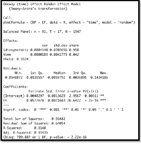
Figure 16 : “Random” time effect model summary between CRP and 1/EF.
Figure 18 : Hausman test for CRP and 1/EF.
In comparison to the model using EF as an explanatory variable, this one explains 31.48% of the variance of CRP, which is 3% more than the previous model. As there is no particular loss of significance in the other indicators, this model can be preferred. The equation is : 𝑪𝑹𝑷𝒊𝒕 = 𝟎. 𝟎𝟎𝟒𝟎 +𝟎.𝟎𝟓𝟕𝟖𝑬𝑭 𝒊𝒕 + 𝑽𝒕+ 𝜺𝒊𝒕 (9) t Vt 2000 -0,0005 2001 -0,0008 2002 0,0038 2003 -0,0028 2004 0,0056 2005 -0,0039 2006 -0,0064 2007 -0,0060 2008 0,0055 2009 -0,0011 2010 -0,0022 2011 -0,0013 2012 -0,0011 2013 0,0014 2014 0,0015 2015 0,0040 2016 0,0045
Table 3 : Random effects per year for all countries using 1/EF.
In the context of this dissertation, this kind of model is more coherent as the lower limit of CRPit is 0, which matches the reality more than the first model because a country risk
premium cannot be lower than 0%. The following graph compares the observations with this model.
Figure 19 : Observations of EF and CRP per year and representation of the “random” model using 1/EF .
6.1.3 Comparison between emerging and developed countries
After these findings, the same process has been repeated four times to analyse separately emerging countries and developed countries (using EF and using 1/EF for each) and compare the results.
To begin with, here is a comparison of the characteristics of the two sets.
Variables n Mean sd Median Min Max Range Skew Kurtosis
CRP 816 0.03 0.03 0.02 0.00 0.18 0.18 1.31 1.67
EF 816 0.44 0.27 0.39 0.06 1.72 1.66 1.45 2.74
Table 4 : Descriptive statistics of the emerging countries dataset.
Variables n Mean sd Median Min Max Range Skew Kurtosis
CRP 731 0.01 0.02 0.01 0.0 0.12 0.12 2.49 6.90
EF 731 5.66 2.17 5.47 1.4 17.72 16.32 1.70 5.97
Table 5 : Descriptive statistics of the developed countries dataset.
Although the mean of CRP for emerging countries is higher than for developing countries (3% against 1%), CRP ranges are similar. On the other hand, the values of ecological footprint are completely different. The average ecological footprint per capita in
developed countries is almost 13 times higher than in emerging countries and the maximal value of EF/capita for emerging countries is slightly higher than the minimal value of EF/capita in developed countries.
• Emerging countries
The analysis of the data regarding emerging countries showed similar results to the full sample. The best model was found using 1/EF as an explanatory variable.
The pooled OLS regression showed a high significance but with a weaker R-squared of 0.1983.
Figure 20 : Pooled OLS regression summary for emerging countries.
The F-stat is lower than for the entire dataset because there are less observations. The p-value is still inferior to 2.22 e-16 which means that the regression is significant to the 0.001 level.
After testing the individual effects models and conducting related tests, the best model ended up to be the “random” model with time effects once more.
Figure 21 : “Random” model with time effect for emerging countries.
Figure 22 : Breusch-Pagan test for time effects for emerging countries
Figure 23 : Hausman test for emerging countries
This set of tests leads to the conclusion that the best model is the “random” model for time effects, although it only explains 20.69% of CRP’s variance. The final equation for the model is :
𝑪𝑹𝑷𝒊𝒕 = 𝟎. 𝟎𝟏𝟑𝟑 + 𝟎.𝟎𝟒𝟏𝟐𝑬𝑭
The values of Vt for emerging countries are the following : t Vt 2000 -2.00e-03 2001 -1.57e-03 2002 3.82e-03 2003 -2.51e-03 2004 8.74e-03 2005 -4.20e-03 2006 -7.97e-03 2007 -7.32e-03 2008 8.18e-03 2009 6.40e-05 2010 -2.18e-03 2011 -2.88e-03 2012 -2.61e-03 2013 1.21e-03 2014 1.48e-03 2015 4.44e-03 2016 5.31e-03
Table 6 : Random effects per year for emerging countries using 1/EF.
• Developed countries
Just as the other samples, the best model for developed countries was the “random” effect model with time effects, but the big difference is that none of the models showed significance when 1/EF was used, which means that the relation that explains best CRP in function of EF is linear.
Figure 24 : “Random” model with time effect for developed countries.
Figure 25 : Breusch-Pagan test for time effect for developed countries.
Figure 26 : Hausman test for developed countries.
Again, the regression and the presence of random time effects are significant to the 0.001 level. This model explains 30.12% of the variance of CRP, its equation is :
𝑪𝑹𝑷𝒊𝒕 = 𝟎. 𝟎𝟒𝟐𝟖 − 𝟎. 𝟎𝟎𝟓𝟐𝑬𝑭𝒊𝒕+ 𝑽𝒕 + 𝜺𝒊𝒕 (11)
The values of Vt for developed countries are the following :
t Vt 2000 3.64e-04 2001 1.39e-04 2002 3.39e-04 2003 -2.87e-04 2004 4.04e-04 2005 -3.56e-04 2006 -5.05e-04 2007 -4.96e-04
2008 4.02e-04 2009 -4.71e-04 2010 -3.45e-04 2011 2.49e-05 2012 -1.85e-05 2013 8.89e-05 2014 3.76e-05 2015 3.47e-04 2016 3.27e-04
Table 7 : Random effects per year for developed countries.
It is now possible to compare emerging countries and developed countries graphically by showing the observations and final models for each.
Figure 27 : Observations of EF and CRP per country development and corresponding models.
6.1.4 Verification of the hypotheses
The first hypothesis was that there was a significant correlation between ecological footprint and country risk premium. The multiple Kendall correlation tests and the
different model regressions emphasized the significant relation between the two variables. All the significant tests and models indicate a negative (or inverse) relation, meaning that CRP decreases or gets closer to 0% as EF increases.
The second and the third hypotheses suggested an effect of time (H2) or country (H3) either fixed or random in the models. After conducting the set of regressions and tests for each samples, the selected model in the end is always the “random” model with time effects, which validates hypothesis H2. The third hypothesis however is rejected as all the tests for country effects, fixed as well as random, were inconclusive.
The last hypothesis implicated a difference in the structure or intensity of the relation depending on the country’s development. The last part of the analysis showed that the R-squared of the final model was a bit weaker for emerging countries than for developing countries, but the main observed difference is in the type of relation. The risk premium for developed countries is best explained by a linear function where it is best explained by an inverse function for emerging countries. As this finding validate hypothesis H4, its first interpretation is that countries with a very low ecological footprint per capita tend to have the highest risk premia and are always emerging countries.
6.2 Interpretation of the results
The analysis of the empirical data indicate a significant negative relation of medium strength between ecological footprint per capita and country risk premium. This result has to be carefully interpreted, as the goal of the dissertation was to emphasize a relation and try to provide evidence for it. After this analysis, it is not possible and would be incorrect to say that increasing the ecological footprint decreases the risk premium of a country. A given country that would purposelessly increase its greenhouse gas emissions as much as possible would increase its ecological footprint per capita in doing so, but cannot possibly expect to lower its risk premium as a consequence. A seemingly more correct way to interpret the highlighted relation is to think of ecological footprint and country risk premium as linked together, as countries with low EF tend to have higher CRP but one is not necessarily the cause of the other.
Another important result is the significant presence of random time effects. As mentioned earlier, the goal of the analysis was not to provide a full explanatory model for country risk premium. There are other variables, probably mostly economic and financial variables that can be used to explain the variance of CRP. This is exactly how the random
time effects should be interpreted. CRP and EF share some explained variance, and a part of the variance that is unexplained has similarities in most of the countries during a given year. This effects are not related in any way to ecological footprint, which is why they are called random effects. Economic and financial events create trends across years, which modify CRP independently from EF, such as the 2008 economic crisis during which most of the developed countries’ CRP rose, creating a random time effect proper to this year.
What this relation means, especially for developed country with a linear relation, is that the process and the drivers that lead to decreasing the country risk premium also leads to increasing the ecological footprint. One can think of it as a cycle. First we know from Borucke et al. (2013) that the ecological footprint of consumption (EFc) is composed of EF for production and trade (EFp and EFt). This means that increases in consumption in general, or production and trade specifically increase the EF. Production, consumption and international trade are factors of economic growth (Ciarli et al., 2010; Makhmutova and Mustafin, 2017) which leads to development and (as the statistic comparison between emerging and developed countries showed) also leads to low risk premia. Hayakawa et
al. (2011) indicate that a low CRP is attractive and leads to higher foreign direct
investment, in debt or equity for the country. The country’s economy becomes richer as investments increase and its potential for production, consumption and trade is increased which generates a higher ecological footprint. This way the cycle of economic growth which leads to lowering the country risk premium also leads to increasing the ecological footprint. This is the way the relation that is put forward in this dissertation should be interpreted. Although Balmford et al. (2002); Braat et al. (2008); Aronson et al. (2010); Blignaut et al. (2014); Sumaila et al. (2017) indicate the long term economic profitability of natural capital conservation and restoration, this dissertation argues that short term economic growth leads doesn’t go without increasing the ecological footprint.
The fact that the data analysis of all the countries and particularly of the emerging countries lead to an inverse relation between EF and CRP directs the attention towards emerging countries and their particular case. The inverse function implies that individuals with the lower values of x (here EF) tend to have unusually higher values for y (CRP) than they should have proportionally (in a linear model for example). It means that countries with very low ecological footprints tend to have extremely high risk premia in comparison to the other countries. As research showed that low risk premia tend to decrease foreign direct investment inflows, and this almost twice more importantly for
emerging countries (Busse and Hefeker, 2005; Hayakawa et al., 2011), the results of this dissertation indicate that investors are attracted to countries with high ecological footprints. It is possible to conclude that these countries are disproportionally less attractive for investors, which with regards to the cycle of economic growth mentioned right before, might actually be preserving their natural capital until solutions for sustainable growth are implemented. This kind of solutions appear in growing numbers, most of them are reported in Parker et al. (2012), but they still need to be applied globally.