Fiscal multipliers and non-separable preferences in a small open economy model

(1)

FISCAL MULTIPLIERS AND NON-SEPARABLE

PREFERENCES IN A SMALL OPEN ECONOMY

MODEL

Nuno Miranda Castanheira

Dissertation submitted as partial requirement for the conferral of

Master in Economics

Supervisor:

Emanuel Gasteiger,

(2)

(3)

Fiscal Policy and Non-separable Preferences

in a Small Open Economy Model

Nuno Miranda Castanheira

⇤

Supervisor: Emanuel Gasteiger, Prof. Auxiliar, ISCTE Business School, Departamento de Economia

Abstract In Euro area countries fiscal policy plays a central role in the stabilization of business cycles mainly because monetary policy is defined for the whole area. A small open economy model is employed to assess the consequences of government expenditure shocks. The main novelty of this thesis is the inclusion of non-separable preferences between private consumption and government expenditure. Numerical simulation suggests that fiscal policy is more e↵ective in a fixed exchange regime. In this regime, fiscal multipliers reach 1.6% on impact and 1% in the long-run.

Resumo Nos pa´ıses da zona Euro a pol´ıtica or¸camental tem um papel chave na estabiliza¸cão dos ciclos económicos principalmente porque a pol´ıtica monetária é definida para o conjunto das economias. Um modelo de pequenas economias abertas é utilizado para avaliar as consequências de um choque nos gastos do governo. O contributo principal desta tese é a introdu¸cão de preferências não separáveis entre o consumo privado e os gastos do Estado. Uma simula¸cão numérica sugere que a pol´ıtica or¸camental é mais eficaz num regime de câmbios fixos. Neste regime, os multiplicadores or¸camentais atingem 1.6% no impacto e 1% no longo prazo.

Keywords: fiscal policy, fiscal multiplier, non-separable preferences, small open economy, exchange rate regime, new Keynesian, DSGE model.

JEL Classification: E62, F41.

(4)

(5)

Acknowledgements

I would like to highlight the role that some people played for the conclusion of this thesis and express my gratitude for all the support received during this crucial year. First of all, and the most relevant for this result, my supervisor Emanuel Gasteiger, without him this thesis wouldn’t have the same end. During this year he provided timely support, deeply looked at every detail and didn’t let me deviate to my hundred ideas. I couldn’t be happier with the choice of my supervisor, I highly recommend him. I would like to thank my macroeconomics professors, Sofia Vale, Vivaldo Mendes and Emanuel Gasteiger for everything they taught me during their classes. They are responsible for all my interest and curiosity in macro subjects. I would also highlight the role of Adriana for all the love she gave me, she has been essential for my success. Her support was unconditional and always motivating. My mother who financed all the university studies. My father who learned about General Equilibrium models than he ever expected he would do and gave useful insights. My sister who encouraged me to apply and have a good result.

Last, but not the least, Nuno da Costa Santos who supervised the estimation of param-eters ↵ and (Subsection 3.2.1) during my 3-month intern at the Office for Strategies and Studies at the Portuguese Ministry of Economy.

(6)

(7)

1 Introduction

1.1 Motivation

The ability of governments to stimulate the economy has been considerably discussed in the literature. Recently, the consequences of the last worldwide crisis and the subsequent coor-dinated stimuli packages (e.g., American Recovery and Reinvestment Act of 2009 (ARRA) and European Economic Recovery Plan (EERP)) came under scrutiny. Articles gauging po-tential e↵ects of government spending on the economy were written and theoretical models were adjusted to empirical findings.

The decision of using countercyclical fiscal policy is usually based on the concept of the fiscal multiplier, i.e., the potential increase in output following an expansion in government expenditures. Moreover, the response of private consumption to a government expenditure shock has played a central role in the discussion because private consumption is the largest component of aggregate demand and consequently the main driver of the multiplier. Further-more, fiscal policy e↵ectiveness is mostly linked to the complementarity or substitutability between private and public expenditures. If public-private consumption are complements, households experience higher utility if both are consumed together. Thus, private consump-tion is likely to increase with a public expenditure shock making fiscal policy e↵ective. Oth-erwise, if substitutes, private consumption would be expected to decrease in response to a government stimulus.

In the aftermath of World War II, worldwide trade experienced a steep growth. Trade agreements, such as GATT, were signed aiming to promote the liberalisation of commerce and the abolition of trade barriers. During the 90’s, the Maastricht Treaty created a single European market. This step led to more integration across economies and to an expansion of international relations inside EU. This development was a key contribution to the glob-alization process and impacted the transmission of fiscal policy.1 _{As a consequence, each}

(10)

time government aims to stimulate economy and purchases goods abroad, there is a leakage of potential benefits to foreign economic agents. In other words, a share of the domesti-cally financed stimulus is very often allocated to imports which, in the end, stimulate other countries. This possibility might induce a free-riding behaviour in countries benefiting from foreign fiscal stimuli. These countries receive a share of others’ fiscal stimulus via higher imports. In the end, this might lead countries to refrain from a larger stimulus. However, it should be highlighted that exports to foreign countries can also play a determinant role o↵setting imports and counter-balance the negative cross-border spillovers. This is why the trade balance is commonly referred as an important instrument to gauge the e↵ectiveness of fiscal policy. As Chinn (2013) and Chen et al. (2013) observe, most open economy models assume countries with a balanced current account. Though, an expansionary stimulus works di↵erently depending whether the economy is balanced or unbalanced.

This investigation begins with a comprehensive literature review aiming to formulate a cutting-edge research question. First, an historical overview is made where earlier fiscal policy in open economy models are revisited. Afterwards is made an exhaustive empirical discussion of fiscal multipliers. Finally, recent theoretical literature is reviewed and short-comings are identified. After having a clear picture of empirical and theoretical literature and being sure of some theoretical gaps that could be improved, a research question emerges. Are non-separable preferences able to properly reproduce empirically documented private-public consumption synchronism? To answer this question, Gal´ı (2008, ch.7) model is augmented with two main novelties: (i) non-separable preferences over private consumption and govern-ment expenditure and (ii) private consumption and governgovern-ment expenditure with asymmetric propensities to import. The model is calibrated to the Portuguese economy. Special atten-tion is given to the calculaatten-tion of the private and public propensities to import. The main purpose of this thesis is to understand the e↵ects of fiscal policy within a small open economy (SOE) and respective interaction with the currency union, similar to Portugal in the context of European Monetary Union (EMU).

(11)

The impulse response functions obtained in the numerical simulation for fixed exchange regime show private consumption and output responding more than one-for-one to an exoge-nous government expenditure shock. The transmission of the fiscal shock is made primarily through private consumption because it is bundled with government expenditure in a non-separable relation. In addition to the non-separability assumption, modelling private con-sumption and government expenditure as complements produces a strong reaction of private consumption. This reaction is strengthened by: (i) the degree of complementarity and (ii) the fixed exchange regime. Moreover, the model confirms a well-known result in the literature, fiscal policy is more e↵ective in the fixed exchange regime. In this regime, fiscal multipli-ers reach 1.6% on impact and 1% in the long-run. In the end, a main policy implication is derived, fiscal stimuli should be directed to sectors with high degree of complementarity relative to private consumption and sectors with low propensity to import to avoid leakages of the stimulus to foreign countries.

1.2 Related Literature

As economies are becoming more interdependent, it is natural to use an open economy model to investigate the consequences of fiscal stimuli. The Mundell-Fleming model, dating from the 60’s, is considered the first step-through to analyse the impact of fiscal policy in open economy context. About two decades later, in the 80’s, the discussion about the e↵ects of government purchases on economy is enhanced with several seminal contributions. Aschauer (1985), Karras (1994), Ni (1995) and Amano & Wirjanto (1998) published articles assessing the relation between private-public consumption but results were mixed and inconclusive. Barro (1981), Aiyagari et al. (1992), Baxter & King (1993) and Finn (1998) built simple neo-classical models to analyse the impact of temporary and persistent increases in government expenditure. According to Real Business Cycle (henceforth RBC) theory, when a govern-ment increases expenditure to stimulate the economy, output increases as well but there is

(12)

consumption) to respond to future tax burdens. To counter-act the decrease in permanent income, households increase labour supply (to increase consumption) but this increment is insufficient to o↵set the wealth e↵ect. RBC theory assumes that government budget is in-tertemporally optimized and debts are always paid. Thus, an increase in current spending will lead to an increase in taxes if not today, tomorrow. This mechanism, commonly referred as Ricardian equivalence, is an implication of most theoretical models assumptions.

Recently, already in the 21st century, these above-cited mainstream contributions were questioned in the light of empirical observations. Empirical literature on fiscal policy is focused at the size of fiscal multipliers, i.e., whether the reaction of GDP exceeds government stimulus. A first step to understand the transmission mechanism of fiscal shocks is to look at the feedback of private consumption to an increase in government expenditures. Blanchard & Perotti (2002), Fat´as & Mihov (2001), Gal´ı et al. (2007), Mountford & Uhlig (2009), Monacelli & Perotti (2010) find private consumption rising after a fiscal stimulus. In particular, Fat´as & Mihov (2001) and Mountford & Uhlig (2009) document long-run fiscal multipliers around 1%. This conclusion supports the Keynesian rather than the neoclassical literature. Perotti (2005) using a panel of OECD countries estimated fiscal policy having a tepid impact on GDP, although, its impact has been rising since 1980’s period. Barro & Redlick (2009), Hall (2009) and Ramey (2011b) estimate fiscal multipliers below or close to one which suggests that fiscal policy is ine↵ective in stimulating economy. Contrary to these findings, Beetsma et al. (2008) and Fisher & Peters (2010) find multipliers higher than one, in particular the authors estimate a peak multiplier of 1.6 and 1.5, respectively. Blanchard & Leigh (2013) and Coenen et al. (2013) assess the recent crisis episode and find that government consumption multipliers larger than one but the e↵ects dissipate once the stimulus is removed. Only one conclusion emerges from this analysis, fiscal multipliers estimates depend on many aspects (e.g., methodology used to identify fiscal shocks and data which might vary in terms of periods or countries). As a result, fiscal multipliers do not converge to a single conclusion and leave the policy maker in trouble. Latest articles about fiscal multipliers focus on specific

(13)

aspects that are worth analysing, such as (i) the degree of openness, (ii) cross-border fiscal spillovers, (iii) the current account balance, (iv) exchange rate regime and (v) business cycles and zero lower bound.

The globalization process that the world has been experiencing has a significant impact in the transmission of fiscal policy. Likewise, fiscal policy e↵ectiveness is also related to the openness of economies and trade diversification. Open economies, depending on the degree of integration, are more vulnerable to foreign economic shocks. Aizenman & Jinjarak (2012) and Ilzetzki et al. (2013) investigated the impact of openness in fiscal multipliers and concluded that economies comparatively closed to trade (”through trade barriers or larger internal markets”2_{) have a fiscal multiplier exceeding one while those more open to trade have}

negative multipliers. Ilzetzki et al. (2013) estimate long-run multipliers in closed economies around 1 percentage point. Beetsma et al. (2008) find closed economies yielding a stronger answer to the stimulus, contrary to open economies where multipliers never exceed 1.

In open economy context, the Ricardian equivalence is not the only argument against expansionary fiscal policy. Unbalanced small open economies with high propensity to import are likely to leak a share of the government stimulus to foreign countries. Thus, an economy with trade surplus can free-ride and benefit from stimuli in other countries. Beetsma et al. (2006) unveiled that cross-border spillovers from a fiscal stimulus would be greater as economies are more integrated, i.e., when they have higher bilateral trade flows. Forni & Pisani (2010) underline that trade leakages tend to be higher immediately after the stimulus as long as the propensity to import expands more than exports multiplier does. Auerbach & Gorodnichenko (2013) found higher spillovers between two countries when both are in recession. Very often, international fiscal spillovers have as transmission channel the current account. Consequently, studying the role of the current account in the transmission of fiscal policy is crucial.

Economies are no longer closed, therefore current account imbalances have a substantial

(14)

impact in the transmission of macroeconomic policies. Countries with an unfavourable trade balance should be cautious with fiscal policy. Although government expenditure is more home-biased than private consumption, the current account response to a fiscal stimulus is still puzzling. It depends on two forces, the complementarity or substitutability between private-public consumption, but also on the characteristics of domestic and foreign goods (e.g., prices and/ or quality). For example, if the government chooses to purchase, in the respective country or abroad, a good which is a complement to private consumption, then private consumption is expected to rise. However, this increment might come from domesti-cally or foreign produced goods depending on the characteristics of the goods in each country. It is not straightforward to conclude whether a fiscal stimulus will lead to an improvement or deterioration of the current account. This uncertainty about the response of the current account is reflected in the empirical studies subsequently presented. Abbas et al. (2011) conclude that a stimulus of 1 percentage point of GDP improves the current account, on impact, in 0.20 percentage points of GDP. However, M. O. Ravn et al. (2012) find fiscal stim-ulus producing a deterioration of trade balance. Kim & Roubini (2008) review the stylized fact of ”twin deficits”, i.e., a pro-cyclical relation between fiscal and current account deficits. The results obtained suggest ”twin divergence”, i.e., when government budget deteriorates, the current account improves. However, Monacelli & Perotti (2010) disagree with this view as their conclusion points towards the so-called ”twin deficit”. In the midway of these two perspectives, Corsetti & M¨uller (2008) find twin deficits more plausible in open economies comparatively to closed economies. The difficulty of measuring the impact of fiscal policy on the current account is clear in these findings.

The transmission of fiscal shocks may still depend on the exchange rate regime. Whether an economy has floating or pegged exchange rate matters a lot for fiscal policy efficacy. Until recently, most theoretical articles assume economies working under a flexible exchange rate regime and empirical research simply ignore the impact of di↵erent exchange rate regimes in fiscal multipliers. The second half of last century has some examples of important fixed

(15)

exchange rate regimes. The Bretton Woods agreement (1944-1971) signed between 45 leading countries established a fixed (but adjustable) exchange rate regime of each currency relative to US dollar. There was also the possibility to convert dollars in gold at a fixed rate. The European Monetary System (EMS), 1979-1998, was based on two mechanisms, the European Currency Union (ECU) and the Exchange Rate Mechanism (ERM) which was itself divided into two instruments, the bilateral exchange rates and the foreign exchange band. In the meantime, European currencies floated relative to US dollar but European central banks manipulated their values. After 1998, the emergence of the EMU put an end to individual monetary and exchange rate policies across Europe creating a single monetary policy and a floating exchange rate relative to US dollar.

The EMU is many times considered a fixed exchange regime. An identical assumption is made in Nakamura & Steinsson (2014) who consider the US economy to be a fixed exchange regime and find fiscal multipliers of 1.5. S. H. Ravn & Spange (2012) examine the impact of fiscal policy in Denmark from 1983 to 2011, a period under currency peg. During this horizon, multipliers reach 1.3 (on impact and cumulative). This means that the stimulus cease once removed. Ilzetzki et al. (2013) found countries with flexible exchange rate having a neutral response to fiscal policy while countries with fixed exchange rates have comparatively higher multipliers. The findings of Corsetti et al. (2012b) and Born et al. (2013) point in the same direction, fiscal multipliers are larger when countries have an exchange rate peg or belong to a currency union.

Conventional macroeconomic theory advocates the use of fiscal policy when all monetary policy benefits are exhausted, that is, as an instrument of last resort. When economic envi-ronment start to deteriorate, the central bank should immediately decrease nominal interest rate to drive down real interest rate making economic agents update their expectations and consequently stimulate private consumption and investment. This should be put in place long before public spending is used as an expansionary measure. Although, the short-term

(16)

When the interest rate reaches zero and monetary policy is not being e↵ective, the economy enters a liquidity trap. Substantial a↵ordable liquidity is available but economic agents do not demand it. This situation is also referred as zero lower bound (ZLB) which is a slowdown time when the traditional monetary policy instruments are ine↵ective.

The Japanese experience over the last two decades motivated research about unconven-tional monetary measures and fiscal policy in liquidity traps. Cutting-edge research supports di↵erent e↵ects of fiscal policy over the business cycle and when the nominal interest rate reaches the zero threshold. Auerbach & Gorodnichenko (2012) look at fiscal multipliers over business cycles and confirmed an impact of more than one-for-one during recessions in com-parison to expansions where the multiplier is situated in the 0-0.5 interval. Similarly, Hall (2009) estimated a 1.7 government purchases multiplier conditional on the ZLB and Owyang et al. (2013) scan slack periods to document multipliers above unity in Canada but below one in the US. Corsetti et al. (2012b) evaluated the impact of financial crises on fiscal mul-tipliers which were estimated to be 2.3 on impact and 2.9 cumulative. Finally, Bachmann & Sims (2012) analyse the impact of fiscal policy on economic agents confidence and found it rising after a public stimulus. In the end, it is concluded that fiscal policy is an appropriate countercyclical tool as output multipliers exceed one.

Over the years, fiscal multipliers have been extensively discussed in the literature. Re-viewing the empirical results leads to the conclusion that literature has a broad range of views to support virtually any policy decision. Ramey (2011a) point that these multiple per-spectives are considered an empirical puzzle as they do not converge to a single transmission mechanism.3 _{The literature does not agree on the size of fiscal multipliers because researchers}

use di↵erent methodologies to identify and estimate the impact of fiscal shocks. Another het-erogeneous issue is that most empirical articles provide estimates for fiscal multipliers but ignore whether they’re impact, peak or cumulative values. Each methodology has drawbacks but two conclusions can be drawn from above: (i) generally private consumption rises after

(17)

a government stimulus (even though its response does not always yield a multiplier higher than one), (ii) fiscal multipliers are higher: in relatively closed economies, in fixed exchange regimes (currency unions), and when monetary policy is constrained by the zero bound.

Despite much debate on the complementarity or substitutability between private con-sumption and government expenditure, a pattern seems to emerge. Most of the times private consumption rises after expansionary fiscal policy. The increase in private consumption af-ter the stimulus suggests a complementarity relation. However, fiscal multipliers are not necessarily higher than unity because the private consumption response might not be strong enough. As pointed out in Karras (1994) government spending has certain types of rival goods (e.g., free-lunches at school) while others are non-rival (e.g., national defence). Although, the author acknowledges that private consumption and public expenditure are, on average, complements. Monacelli & Perotti (2010) suggested to upgrade open economy models with a mechanism generating a positive response of private consumption whenever the govern-ment stimulates economy. One way to embed this suggestion is to include non-separable preferences over private consumption-leisure or private-public consumption. The latter case makes households’ utility dependent on a bundle of private-public consumption, referred as e↵ective consumption in the literature. Although both types of (private and public) consump-tion a↵ect households’ utility, households only choose the amount of private consumpconsump-tion. Moreover, private consumption and government expenditure might be complements or sub-stitutes depending on the calibration of the parameters. This relation has a profound impact in the e↵ectiveness of fiscal policy. If government stimuli are directed to goods which are complements to private consumption, then fiscal policy is likely to be e↵ective as private con-sumption is crowded-in. On the other hand, if government expenditure substitutes private consumption, fiscal policy is not expected to succeed. A relevant research question would be whether non-separable preferences are able to properly reproduce empirically documented private-public consumption synchronism?

(18)

the shortcomings of Mundell-Fleming model. Obstfeld & Rogo↵ (1995), as precursor of NOEM, developed a perfect-foresight two-country general equilibrium model with imperfect competition and nominal rigidities in the goods and labour markets. Since then, two-country models evolved and gave origin to new Keynesian SOE models. Gal´ı & Monacelli (2005) built a model where it is assumed a world economy populated by infinite small open economies. Afterwards, Gal´ı & Monacelli (2008) developed this model to accommodate for fiscal policy and study its consequences in a SOE context. Along this article authors analyse the conse-quences of a fiscal stimulus in a currency union. The same is done in Ferrero (2009) but in a two-country framework. In the last years, theoretical models have been improved and com-plemented with relevant features such as: (i) rule-of-thumb consumers4_{, (ii) habits in private}

consumption5_{, (iii) the e↵ect of zero lower bound}6 _{and (iv) non-separable preferences.}

Following the suggestion of Monacelli & Perotti (2010), some authors incorporate non-separable preferences in theoretical models as a mechanism to generate a positive response of private consumption to government expenditure shocks. Non-separable preferences are included in theoretical models through two common ways, an Edgeworth mechanism or a constant elasticity of substitution (CES) index7_{. For example, private consumption and}

government expenditure are usually bundled in a new variable, the e↵ective consumption which is represented as follows

Edgeworth mechanism: bCt⌘ (1 #)Ct+ #Gt,

CES: bCt⌘

⇥

(1 #)C_t1 ⌫ + #G1 ⌫_t ⇤1 ⌫1 _.

Cortuk (2013), Bouakez & Rebei (2007), Linnemann & Schabert (2004) and Ercolani &

4_{Among relevant literature on rule-of-thumb consumers see Coenen & Straub (2005), Coenen et al. (2013)}

Gal´ı et al. (2007) and Forni & Pisani (2010).

5_{Several recent articles introduce habits in private consumption such as Bouakez & Rebei (2007), F`eve &}

Sahuc (2013), Coenen et al. (2013) and M. O. Ravn et al. (2012).

6_{For a representative perspective of recent theoretical literature about fiscal policy at ZLB see, among}

others, Christiano et al. (2011), Farhi & Werning (2012), Correia et al. (2013), Erceg & Lind´e (2014), Fujiwara & Ueda (2013) and Ercolani & Azevedo (2013).

(19)

Azevedo (2013) use closed economy models with CES non-separable preferences to evaluate fiscal policy outcomes. The first three assume complementarity while the last considers substitutability. Cortuk (2013) instead of using a non-separable relation between private consumption and government purchases as the others, use government production. Ganelli & Tervala (2009) also employ a closed economy paradigm but introduce non-separability via Edgeworth complementarity. Bilbiie (2011) evaluate fiscal policy in a closed economy model with non-separable preferences over private consumption and leisure.

Ganelli (2003), Tervala (2005) and Iwata (2013) apply the Edgeworth mechanism in open economy models to explore the relation between private-public consumption. The first two use the Obstfeld-Rogo↵ (also called OR) framework and assume substitutability. Though, the last use an alternative two-country framework with complementarity assumption.

Finally, an analysis of the literature above leads to the conclusion that open economy models augmented with non-separable preferences are relatively scarce. Moreover, there is no new Keynesian SOE model measuring the impact of fiscal policy in a fixed exchange regime under non-separability. Furthermore, discussing the linkages of fiscal policy within each exchange rate regime is of interest. Particularly, in currency unions fiscal spillovers is a topic of special concern because stimuli can easily flood to neighbouring countries depending on the propensity to import. Afterwards, fiscal policy in fixed exchange regime is studied using a SOE model.

The remainder of the article is structured as follows: Section 2 describes the structure of a new Keynesian SOE model with non-separable preferences over private consumption and government expenditure. In Section 3, the model is calibrated and results from a numeri-cal simulation are discussed. Finally, Section 4 concludes and points directions to further research.

(20)

(21)

2 The Model

This section elaborates Gal´ı (2008) model8_{incorporating three main novelties: (i) government}

expenditure in the utility function, (ii) non-separable preferences over private consumption and government expenditure and (iii) private consumption and government expenditure with asymmetric propensities to import. The model assumes a world economy made of a contin-uum of infinitesimally SOE’s distributed along the [0,1] interval. The SOE framework is also used in previous research such as Gal´ı (2008), Gal´ı & Monacelli (2008) and Benigno & De Paoli (2010). An assumption of the model is that preferences, market structure and tech-nology except productivity shocks are equal across economies. As pointed out in Benigno & De Paoli (2010, p.1524), ”The [small open] economy is perfectly integrated with the rest of the world that is, there are no trade frictions (i.e., the law of one price holds) and capital markets are perfect (i.e., asset markets are complete).” Market completeness also implies that marginal utilities are identical in every period and all countries.

2.1 Households

Each and every SOE has a representative household maximizing intertemporal utility. The utility function is made of two components, e↵ective consumption ( bCt) and hours of work

(Nt), E0 1 X t=0 t_U⇣_C_b t, Nt ⌘ = E0 1 X t=0 t Cbt1 1 N_t1+' 1 + ' ! , (2.1)

where 1 _{> 0 is the Arrow-Pratt measure of relative risk aversion and the inverse of the}

intertemporal elasticity of substitution, ' is the inverse of the Frisch elasticity of labour supply and is the subjective time discount factor. E↵ective consumption is a composite index of private consumption (Ct) and government expenditure (Gt). A non-separable

re-lation between private and government consumption is assumed, i.e., the utilities of private consumption and government expenditure are no longer independent. An increase in

(22)

gov-ernment expenditures leads to an increase (decrease) of private consumption if complements (substitutes). One of the first studies using non-separable preferences over private and public consumption was Amano & Wirjanto (1998). Such specification is also used in Bouakez & Rebei (2007), Coenen et al. (2013) and Cortuk (2013). E↵ective consumption is given by

b Ct⌘ 8 > > < > > : ⇥ (1 #)C_t1 ⌫ + #G1 ⌫_t ⇤1 ⌫1 _{, for ⌫} _{6= 1,} C_t(1 #)G# t, for ⌫ = 1. (2.2)

The parameter ⌫ 1 _{> 0 defines the intratemporal complementarity or substitutability}

be-tween private consumption and public expenditure and is one of the key parameters for the magnitude of the fiscal multiplier, as well as . In the case public-private consumption are considered complements, an increase in one produces an increase in the other while if sub-stitutes, a fiscal stimulus would crowd-out private consumption and make fiscal policy less e↵ective or even ine↵ective. Following Amano & Wirjanto (1998): if 1 _{> ⌫} 1_{, private}

consumption and government expenditure are Edgeworth-Pareto complements; if 1 _{< ⌫} 1_,

then private-pubic consumptions are Edgeworth-Pareto substitutes; and finally if 1 = ⌫ 1, then the goods are unrelated. This last equality also implies that preferences are additively separable in private and public consumption.

The log-linearisation of the system of equations (2.2) take the form

bct⌘ 8 > > < > > : (1 #) ✓ C b C ◆1 ⌫ ct+ # ✓ G b C ◆1 ⌫ gt, for ⌫ 6= 1, (1 #)ct+ #gt, for ⌫ = 1, (2.3)

where C, G and bC are the steady state values of private, public and e↵ective consumption, respectively.9 _{Inside e↵ective consumption index, b}_C

t, there are two additional sub-indexes,

Ct and Gt. The private consumption index is exactly equal to the one presented in Gal´ı &

(23)

Monacelli (2005) and Gal´ı (2008), Ct = h (1 ↵)1⌘ (C H,t) ⌘ 1 ⌘ + ↵1⌘(C F,t) ⌘ 1 ⌘ i ⌘ ⌘ 1 . (2.4)

As above, the complementarity or substitutability between types of consumption is critical to the size of the fiscal multiplier. The same happens in what respects to the relation between domestically and foreign produced goods. If these are complements, an increase of domestic private consumption will lead to an expansion of imports. Whereas if they are substitutes, the reverse happens.

One of the novelties in this work is to assume that government spending has a similar structure to private consumption. Now, contrary to Gal´ı & Monacelli (2008) and Forni & Pisani (2010), there is no home bias in government expenditure, a fraction ( ) is purchased abroad. Gt= h (1 )1⌘(G H,t) ⌘ 1 ⌘ ₊ 1⌘ (G F,t) ⌘ 1 ⌘ i ⌘ ⌘ 1 . (2.5)

Private consumption and government expenditure are assumed to share a similar composi-tion. Constant elasticity of substitution (CES) functions are used to aggregate a large sum of goods/varieties into just one.10 _C

H,t and GH,t are indexes representing a basket of

domes-tically produced goods which have as many j varieties as the numbers in the interval [0,1], i.e., a continuum of di↵erentiated varieties.

CH,t⌘ ✓Z 1 0 CH,t(j) " 1 " dj ◆ " " 1 and GH,t ⌘ ✓Z 1 0 GH,t(j) " 1 " dj ◆ " " 1 ;

On the other hand, imports depend not only on j varieties produced abroad but also on i countries of origin. CF,tand GF,t are indexes measuring the quantity of imported goods from

10_{Constant elasticity of substitution aggregators are very often referred as Armington aggregators or}

(24)

each country. For instance, how much does Portugal import from each country? CF,t ⌘ ✓Z 1 0 (Ci,t) 1 di ◆ 1 and GF,t⌘ ✓Z 1 0 (Gi,t) 1 di ◆ 1 ;

While, Ci,t and Gi,t measure the composition of imports in terms of varieties imported from

each country i. Which is the structure of the Portuguese imports from Spain? From which sectors does Portugal import?

Ci,t ⌘ ✓Z 1 0 Ci,t(j) " 1 " dj ◆ " " 1 and Gi,t ⌘ ✓Z 1 0 Gi,t(j) " 1 " dj ◆ " " 1 ;

Note that the goods purchased by the government and private sector are the same, and consequently there is just one domestic price (PH,t) and one foreign price (PF,t). Although,

there might be di↵erent propensities to import, i,e., ↵ _{6= .}

Take into consideration that #_{2 [0,1] is the percentage of government spending in e↵ective} consumption and ⌫ is the inverse of the intratemporal elasticity of substitution between private consumption and government spending. Parameters ↵ and _{2 [0,1] measure the} shares of imported goods of private consumption and government expenditure, respectively. " > 1 is the Dixit-Stiglitz parameter for within-country consumption, ⌘ > 0 stands for the elasticity of substitution between domestically and foreign produced goods whereas accounts for the substitutability between goods produced in di↵erent foreign countries.

The households budget constraint is given by

P_tCCt+ Et{Qt,t+1Dt+1}  Dt+ WtNt+ Tt, (2.6) where PC t ⌘ ⇥ (1 ↵) (PH,t)1 ⌘+ ↵ (PF,t)1 ⌘ ⇤ 1

1 ⌘ _{is the CPI and C}

tis the private consumption

index, as in (2.4). Dt ”is the nominal payo↵ in period t+1 of the portfolio held at the end of

period t (and which includes shares in firms)”11_{, W}

t is the nominal wage paid to every hour

(25)

worked by the household, Tt are lump-sum transfers which do not a↵ect incentives to work,

save or invest and Qt,t+1 ”is the stochastic discount factor for one-period-ahead nominal

payo↵s relevant to the domestic household”11. In this model, the small open economies have the property of perfect and complete financial markets, which implies the existence of a worldwide traded security. Total private consumption expenditures in domestically and foreign produced goods is given by PC

t Ct= PH,tCH,t+ PF,tCF,t.12

The representative household of each SOE maximizes lifetime utility subject to a stream of budget constraints.13 _{The optimality conditions are obtained maximizing households utility}

controlled by the budget constraint. The intratemporal optimality equation is given by Wt

PC t

= (1 #) 1N_t'C_t⌫Cb_t ⌫. (2.7)

Whereas, the intertemporal optimality equation (often called Euler equation) takes the form

Et (✓ Ct+1 Ct ◆ ⌫ _b Ct+1 b Ct !⌫ ✓ PC t PC t+1 ◆) = Qt, (2.8) where Qt= Et{Qt,t+1}.

The above expressions are log-linearised with respect to their steady state values as follows

wt pCt = 'nt+ ⌫ct+ ( ⌫)bct, (2.9) = 'nt+ ct+ (⌫ ) (ct bct) , (2.10) ct= Et{ct+1} 1 ⌫ it Et ⇡ C t+1 ⇢ + ⌫ ⌫ (Et{bct+1} bct) , (2.11) = Et{ct+1} 1 it Et ⇡Ct+1 (⌫ ) Et{(ct+1 bct+1) (ct bct)} ⇢ , (2.12) 12_PC

t is identical to Ptin Gal´ı (2008) but now there is a price index for private consumption and other for

the government expenditure.

13_{This section follows the derivation of the budget constraint in the book Gal´ı (2008) and Gal´ı & Monacelli}

(26)

where lower case letters represent the logs of the respective variables, Et ⇡Ct+1 = Et pCt+1

pC

t is CPI inflation14 (with pCt ⌘ log PtC), it ⌘ log Et{Qt,t+1} is short-term nominal interest

rate and ⇢ ⌘ log is the steady state time discount rate.

2.2 Government

Taking into consideration that the government expenditure shares the same structure of private consumption, the government budget constraint is derived in a similar way to the households budget constraint. Through comparison to Appendix A.2, the government budget constraint is easily obtained15

P_tGGt+ Et{Qt,t+1Dt+1}  Tt+ Dt, (2.13) where PG t ⌘ ⇥ (1 ) (PH,t)1 ⌘+ (PF,t)1 ⌘ ⇤ 1

1 ⌘ _{is the government price index, henceforth}

GPI and Gt is the government expenditure index as in (2.5). The remaining variables are

identical to those in the households constraint. For simplicity it is assumed that government does not use bonds to finance expenditures, has a balanced budget in each and every period. Then equation (2.13) might be re-written as follows

P_tGGt  Tt. (2.14)

Note that if ↵ = , then PC

t = PtG = Pt, that is if private and public sectors have the same

propensity to import, there is just one price index, identical to the one in Gal´ı (2008). In this model, domestic and world government expenditure are exogenous, expressed in

14_{More details in Section 2.3 below.}

(27)

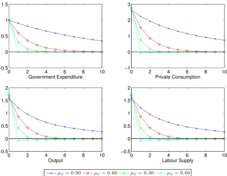
log-deviation from the steady state and defined as an autoregressive process.16 gt= ⇢ggt 1+ "gt, where " g t i.i.d. ⇠ N (0, "g_t), (2.15) g_t⇤ = ⇢g⇤g⇤_{t 1}+ "g ⇤ t , where "g ⇤ t i.i.d. ⇠ N (0, _"g⇤ t ), (2.16)

where ⇢g and ⇢g⇤ 2 [0,1] are the autocorrelation parameters accounting for the persistence

of the shock whereas "g_t and "g_t⇤ represent the shocks to the domestic and world government expenditure, respectively. Note that if ⇢g = 1 the increase in government expenditures would

be perpetual whereas if ⇢g = 0 the shock would last one period only.

2.3 Prices

The present section describes several hypotheses of the model which are regularly used below. It follows closely the definitions presented in Gal´ı (2008). First of all, the bilateral terms of trade are expressed as Si,t =

Pi,t

PH,t

and refer to the ratio of country i price index (measured in domestic currency) relative to the home country price index. Likewise, the e↵ective terms of trade are given by

St= PF,t PH,t = ✓Z 1 0 S 1 i,t ◆ 1 1 . (2.17)

The terms of trade in log-deviations from its steady state value is given by

st⌘ log St=

Z 1 0

si,tdi = pF,t pH,t. (2.18)

CPI is log-linearised assuming a symmetric steady state as follows

pC_t _{⌘ (1} ↵)pH,t+ ↵pF,t= pH,t+ ↵st. (2.19)

16_{Identical specification of fiscal shocks can be found in Linnemann & Schabert (2004), Coenen & Straub}

(28)

and domestic CPI inflation is given by

⇡C_t _{⌘ p}C_t pC_{t 1}= (1 ↵)⇡H,t+ ↵⇡F,t= ⇡H,t+ ↵ st. (2.20)

Similarly, the linearisation of GPI yields

pG_t _{⌘ (1} )pH,t+ pF,t= pH,t+ st (2.21)

and domestic GPI inflation is

⇡G

t ⌘ pGt pGt 1 = (1 )⇡H,t+ ⇡F,t= ⇡H,t+ st. (2.22)

An important assumption of this model is that the law of one price holds for every variety of goods j 2 [0,1], implying the immediate translation of any foreign price variation into the domestic country through its imports. In other words, there is a complete exchange rate pass-trough to import prices in every time horizons or there are no trade frictions. Prices of each good j in the foreign country i measured in foreign currency, Pi

i,t(j), are transformed

into country i’s prices in domestic prices through the bilateral nominal exchange rate, _Ei,t.

This is equivalent to say that the following expression Pi,t(j) =Ei,tPi,ti (j) hold for each good

j _{2 [0,1]. Furthermore, if this identity hold for individual goods, it is also valid for the} aggregate, i.e., Pi,t =Ei,tPi,ti . Where Pi,t ⌘

⇣R1 0 Pi,t(j)

1 "_dj⌘ 1 1 "

is the country i’s price index for all varieties of goods measured in domestic currency and Pi

i,t ⌘ ⇣R1 0 Pi,ti (j)1 "dj ⌘ 1 1 " is the country i’s aggregate price index in their own currency. Recall that PF,t ⌘

⇣R1 0 P 1 i,t di ⌘ 1 1 . Plugging the law of one price for each economy i (instead of being for each good j) in the last equation and then log-linearising around the symmetric steady state, yields the following

pF,t =

Z 1 0

(29)

where et⌘

R1

0 ei,tdi is the e↵ective nominal exchange rate in log-deviations from the steady

state and p⇤ ⌘R01pii,tdi is the log of world price index. Any time there is a superscript with

an asterisk, it denotes the integration over every country i 2 [0,1], that is world variables. Notice that, for the latter case, as it is a price index for the whole world, there is no di↵erence between CPI (or GPI) inflation and domestic inflation17_{. The last result might be combined}

with the terms of trade, equation (2.18) and yields18

st= et+ p⇤t pH,t. (2.23)

Households bilateral real exchange rate is given by

QC i,t = PtC,iEi,t PC t = P C i,t PC t , (2.24)

which, if linearised, can be expressed as

q_tC ⌘ log QC i,t = Z 1 0 q_i,tCdi = Z 1 0 ⇣ ei,t+ pC,it pCt ⌘ di, = et+ pC,t ⇤ pH,t+ pH,t pCt + p⇤t p⇤t, = st+ pH,t pCt + p C,⇤ t p⇤t, = (1 ↵) st+ ⇣ pC,⇤t p⇤t ⌘ . (2.25)

Looking closer at what is ⇣pC,_t ⇤ p⇤ t

⌘

, one may conclude that it cancel out becauseR₀1si tdi =

0, for instance Gal´ı (2008, p.161), thus

pC,⇤t = Z 1 0 pC,it di = Z 1 0 (pi_i,t+ ↵si_t)di = p⇤_t. (2.26)

17_{For a detailed demonstration of this result, check equation (2.26).}

18_{In the simulation of the model is used a di↵erenced version of equation (2.23) as follows}

(30)

In words this means that the world consumer price index (pC,⇤t ) is the integration of all

economies consumer price indexes (R₀1pC,it di). In turn, each country consumer price index

(pCt ) is made of its respective domestic price index (pH,t) and the propensity to import times

the terms of trade (↵st). Next, the log-linearisation ofQCi,t yields

qC_t ⌘ (1 ↵) st. (2.27)

Similarly, the government bilateral real exchange rate is

QGi,t = PtG,iEi,t PG t = P G i,t PG t . (2.28) which yields q_tG_{⌘ (1} ) st. (2.29)

Again, note that if ↵ = all this analysis collapses to equations (2.30) and (2.31) where there is only one bilateral real exchange rate, _Qi,t. The e↵ective bilateral real exchange rate

becomes the ratio of the two countries price indexes, both expressed in terms of domestic currency Qi,t = Pi tEi,t Pt = Pi,t Pt . (2.30)

The log e↵ective real exchange rate is given by

qt ⌘ Z 1 0 qi,tdi = Z 1 0 ei,t+ pit pt di, = et+ p⇤t pH,t+ pH,t pt, = st+ pH,t pt, (2.31)

(31)

2.4 International Risk Sharing

The common approach in the SOE framework is to assume complete financial markets. The return on a cross-border security influences the intertemporal allocation of households’ bud-get. The ratio current vs. future consumption depends on the expected return of the security. Country i’s intertemporal optimization equation (in terms of domestic currency) is given by

✓ Ci t+1 Ci t ◆ ⌫ _b Ci t+1 b Ci t !⌫ ✓ Ei,t Ei,t+1 ◆ P_tC,i P_t+1C,i ! = Qt. (2.32)

Expressions (2.8) and (2.32) may be combined in order to derive the equilibrium condition for the internationally traded security. In equilibrium, it holds such that

C_t⌫Cb_t ⌫ = $i Cti ⌫⇣_b

C_ti⌘ ⌫_QC_i,t, (2.33)

where $i is a constant characterizing the relative composition of the balance sheet of each

country. Log-linearising (2.33), integrating over [0,1] and having in mind that in aggregate $i = $ = 1, i.e., zero net foreign asset holdings, one can derive

⌫ct+ ( ⌫)bct= ⌫c⇤t + ( ⌫)bc⇤t + qtC, (2.34) ct= c⇤t + ⌫ ⌫ (bc ⇤ t bct) + 1 ↵ ⌫ st, (2.35) where c⇤_t = R₀1ci

tdi is the (log) index for world private consumption and bc⇤t =

R1

0 bcitdi is

linearised expression for the e↵ective world consumption. The complete markets hypothesis allows having an identity as (2.35) relating private and e↵ective world consumption to the terms of trade (st) and the degree of openness (↵).

(32)

2.5 Firms

2.5.1 Production Function

Every firm in this model uses labour (Nt) and technology (At) to produce a di↵erentiated

good j 2 [0,1]. The production function of each firm (or good) does not include physical capital for simplicity19 _{and is expressed as follows}

Yt(j) = AtNt(j), (2.36)

where technology follows an AR(1) process, at= log At= ⇢aat 1+"t. The linearisation of the

aggregate production function is given by yt= at+ nt. Solving the typical firms optimization

problem20 one obtains an expression for the real marginal cost, which is identical to every firm

mct = + wt pH,t at, (2.37)

where _{⌘ log(1} ⌧ ) is a employment subsidy.

2.5.2 Price Setting

The model sets prices according to Calvo (1983), i.e., are adjusted in a staggered manner. In this framework, similar to Gal´ı (2008), a fraction of firms are selected to re-optimize profits changing prices with regard to new contingencies. In other words, selected firms maximize the expected discounted profits. The probability of being selected to re-optimize is timely-independent of the last pricing decision. The price index resulting from this property is given by pH,t = µ + (1 ✓) 1 X k=0 ( ✓)kEt{mct+k+ pH,t+k} , (2.38)

19_{For a similar model with capital see Gal´ı et al. (2007).}

(33)

where ✓ 2 [0, 1]. Every period a share (1 ✓) of randomly selected firms are able to set new prices while the remaining share ✓ have to keep their prices fixed. Consider also that µ⌘ log

✓ " " 1

◆

is the equilibrium markup in the flexible price state. This assumption leads to the inflation equation

⇡H,t = Et{⇡H,t+1} + mcct, (2.39)

where _⌘ (1 ✓)(1 ✓)

✓ is a coefficient that relates the probability of resetting prices with the time discount rate.21

2.6 Equilibrium

2.6.1 The Demand Side

The demand side of this economy has two economic agents, the households and the govern-ment. Each consumes a certain quantity of each good variety j which need to be aggregated to obtain the demand for the whole economy. An assumption of this model is that goods market clear every period.

The demand of country i for good j is made of two parts, the domestic production which is domestically consumed but also the foreign production domestically consumed, i.e., the imports of each good j from each country i. The demand of good j in each country i is then defined as Yt(j) = (1 #) ✓ PH,t(j) PH,t ◆ "" (1 ↵) ✓ PH,t PC t ◆ ⌘ Ct+ ↵ Z 1 0 PH,t Ei,tPF,ti ! ✓_Pi F,t PtC,i ◆ ⌘ C_tidi # +# ✓ PH,t(j) PH,t ◆ "" (1 ) ✓ PH,t PG t ◆ ⌘ Gt+ Z 1 0 PH,t Ei,tPF,ti ! ✓ Pi F,t P_tG,i ◆ ⌘ Gi tdi # . (2.40) This equation is similar to equation (24) in Gal´ı (2008, p.160) but with two novelties, first government consumption is added to the demand for good j and second, each type of

(34)

con-sumption (private or public) has its own price, PC

t and PtG.

Aggregate demand of each country i is the sum of every demand for each good variety j. Consequently, aggregate demand of each country i is the integration over [0,1] of the demand for each product type as Yt⌘

hR1 0 Yt(j) " 1 " dj i " " 1

. Integrating expression (2.40) yields

Yt = (1 #) " (1 ↵) ✓ PH,t PC t ◆ ⌘ Ct+ ↵ Z 1 0 PH,t Ei,tPF,ti ! ✓_Pi F,t PtC,i ◆ ⌘ C_tidi # +# " (1 ) ✓ PH,t PG t ◆ ⌘ Gt+ Z 1 0 PH,t Ei,tPF,ti ! ✓_Pi F,t P_tG,i ◆ ⌘ Gi_tdi # . (2.41)

Making some arithmetic operations, which are detailed in Appendix A.11, results in

Yt = (1 #) ✓ PH,t PC t ◆ ⌘" (1 ↵)Ct+ ↵ Z 1 0 ✓_E i,tPF,ti PH,t ◆ ⌘ QCi,t ⌘ C_tidi # +# ✓ PH,t PG t ◆ ⌘" (1 )Gt+ Z 1 0 ✓_E i,tPF,ti PH,t ◆ ⌘ QGi,t ⌘ Gi_tdi # . (2.42)

Equation (2.33) can be used to simplify (2.42), i.e.,

Yt= (1 #) ✓ PH,t PC t ◆ ⌘ Ct 2 4(1 ↵) + ↵Z 1 0 S i tSi,t ⌘ QCi,t ⌘ 1_⌫ Cbt b Ci t ! ⌫ ⌫ di 3 5 +# ✓ PH,t PG t ◆ ⌘ (1 )Gt+ Z 1 0 S i tSi,t ⌘ QG i,t ⌘ Gitdi , (2.43) where_Si

t stands for e↵ective terms of trade for country i andSi,t is the bilateral terms of trade

between the home economy and country i, identical to Gal´ı (2008). To have a manageable solution for this model the last expression is first-order log-linearised around a symmetric steady state and integrated. Moreover, recalling that R₀1si

tdi = 0, one has yt = (1 #)  ⌘ pH,t pCt + ct+ ↵  ( ⌘) st+ ✓ ⌘ 1 ⌫ ◆ qC_t + ✓ ⌫ ⌫ ◆ (_bct bc⇤t) +#⇥ ⌘ pH,t pGt + (1 )gt+ ⇥ ( ⌘) st+ ⌘qtG+ gt⇤ ⇤⇤ , (2.44)

(35)

where bct is the log-linearised e↵ective consumption, bc⇤t is the world e↵ective consumption

and g_t⇤ is the world government expenditure. Substituting the following simplifications !C _⌘

⌫ + (⌘⌫ 1) (1 ↵) and !G ⌘ ⌫ + ⌘⌫ (1 ), the last expression becomes

yt = (1 #)  ct+ ↵ ⌫! C_s t+ ↵ ✓ ⌫ ⌫ ◆ (_bct bc⇤t) + # h (1 )gt+ ⌫! G_s t+ gt⇤ i . (2.45)

Taking into consideration that R₀1si

tdi = 0, world output is given by

y_t⇤ = (1 #)c⇤_t + #g⇤_t, (2.46)

where c⇤_t is world private consumption. Isolating st, substituting ⌥ = (1 #)

↵ ⌫(! C _{1) +} # ⌫! G₊ (1 #)

⌫ and also the world output, equation (2.45) turns into yt = yt⇤+ (1 #)  (1 ↵) ✓ ⌫ ⌫ ◆ (bc⇤t bct) + # [(1 ) (gt gt⇤)] + ⌥st. (2.47)

Combining the Euler equation (2.11) with equation (2.45) yields

yt = Et{yt+1} ⌥ (it Et{⇡H,t+1} ⇢) h ⇤ + ⌫ (1 #) i # ✓ ⌫ 1 # ◆ Et gt+1⇤ + ⇤ ✓ ⌫ 1 # ◆ Et y⇤t+1 (1 )#Et{ gt+1} + h ⇤ + ↵ ⌫ (1 #) i ( ⌫) Et bc⇤t+1 h ⌥ + ⇤ + ↵ ⌫ (1 #) i ( ⌫) Et{ bct+1} , (2.48) where ⇤ ⌘ ⌥ 1 # ⌫ = h (1 #)↵ ⌫(! C _{1) + #} ⌫! Gi_{, and y} t is log-linearised aggregate demand.

Finally, net exports are expressed in deviations of the steady state output Y22

nxt= N Xt Y ⇡ 1 Y  Yt PC t PH,t Ct PG t PH,t Gt .

(36)

After applying a first order linear approximation to the last equation, one has

nxt= yt (1 #) (ct+ ↵st) # (gt+ st) , (2.49)

which, if combined with equation (2.45), yields

nxt = (1 #)  ↵ ✓ !C ⌫ 1 ◆ st+ ↵ ✓ ⌫ ⌫ ◆ (_bct bc⇤t) + #  ✓ !G ⌫ 1 ◆ st+ (g⇤t gt) . (2.50)

2.6.2 The Supply Side

A first step to obtain the natural level of output is to get the flexible prices marginal cost. In order to obtain it, one has to make some transformations in the optimal real marginal cost expression derived in Section 2.5

mct= + wt pH,t at, (2.37)

mct= + 'yt+ ⌫c⇤t + ( ⌫)bc⇤t + st (1 + ') at, (2.51)

which makes use of equations (2.9), (2.19), (2.35) and the linearised production function. Using (2.47) to replace st above produces

mct = + ✓ ⌥' + 1 ⌥ ◆ yt 1 ⌥y ⇤ t + ⌫c⇤t + ✓ ⇤ + ↵ ✓ 1 # ⌫ ◆◆ 1 ⌥( ⌫)bc ⇤ t (1 + ') at + (1 ↵) ✓ 1 # ⌫ ◆ 1 ⌥( ⌫)bct #(1 ) 1 ⌥gt+ #(1 ) 1 ⌥g ⇤ t. (2.52)

Under flexible prices the marginal cost is constant, mct = µ. The natural level of output

is represented by

(37)

where 0 ⌘  ⌥ ( µ) ⌥' + 1 , y⇤ ⌘  1 ⌥' + 1 , c⇤ ⌘  ⌥⌫ ⌥' + 1 , bc⇤ ⌘  ⇤ + ↵ ✓ 1 # ⌫ ◆ ✓ 1 ⌥' + 1 ◆ ( ⌫), _bc_⌘ ✓ 1 # ⌫ ◆  1 ↵ ⌥' + 1 ( ⌫), g ⌘  #(1 ) ⌥' + 1 , g⇤ ⌘  #(1 ) ⌥' + 1 , a⌘  ⌥ (1 + ') ⌥' + 1 . 2.6.3 The Equilibrium Dynamics

Having in mind that the output gap is defined by

˜

yt ⌘ yt ytn, (2.54)

one can start by substituting (2.53) into (2.54), and finally using the resulting expression to substitute into (2.52) generates a relation between the output gap and the steady state (i.e., flexible prices) domestic real marginal cost

c mct= ✓ ' + 1 ⌥ ◆ ˜ yt. (2.55)

If the last equation is used to substitute in (2.39) the new Keynesian Phillips curve (NKPC) is obtained as ⇡H,t= Et{⇡H,t+1} + ↵y˜t, (2.56) where ↵ ⌘ ✓ ' + 1 ⌥ ◆

is the slope coefficient.23

To obtain the dynamic IS equation for the open economy in terms of the output gap one has to start with the IS equation (2.48), then substitute the output gap (2.54) and finally

23_{Please notice that when }

(38)

replace (2.53) which yields ˜ yt= Et{˜yt+1} ⌥ (it Et{⇡H,t+1} rtn)  ⌥ + ⇤ + ✓ 1 # ⌫ ◆ ✓ ↵⌥' + 1 ⌥' + 1 ◆ ( ⌫) Et{ bct+1} , (2.57) where rn

t is the natural (or Wicksellian) rate of interest of the domestic economy and has the

following format rn_t _{⌘ ⇢ +}  ⇤ ✓ ⌫ 1 # ◆ + 1 ⌥' + 1 1 ⌥Et y ⇤ t+1  ⌫ ⌥' + 1 Et c ⇤ t+1  ' ⌥' + 1 (1 )#Et{ gt+1} + h ⇤ +↵ ⌫ (1 #) i ✓ _' ⌥' + 1 ◆ ( ⌫) Et bc⇤t+1  ⇤ ✓ ⌫ 1 # ◆ + + 1 ⌥' + 1 # 1 ⌥Et g ⇤ t+1  (1 + ') ⌥' + 1 (1 ⇢a) at. (2.58) As already emphasized, the current model is based in Gal´ı (2008, ch.7) open economy model. For # = 0, ↵ = and = ⌫ the model is identical to Gal´ı (2008, ch.7). Additionally, if ↵ = 0, the model becomes a closed economy as in Gal´ı (2008, ch.3). In the end, it is possible to conclude that this model nests both Gal´ı (2008) models.

(39)

3 Numerical Simulation

3.1 The Policy Experiment

The present section quantitatively analyses the results of a government expenditure shock in the model above elaborated. As referred earlier, fiscal policy is modelled as an exogenous government expenditure shock. Recall also that government expenditure is modelled through an autoregressive process as follows

gt= ⇢g gt 1+ "gt, where " g t

i.i.d.

⇠ N (0, "g_t). (2.15)

In the simulation of the model, both fixed and flexible exchange rate regimes are scrutinized in order to derive relevant policy implications. Each regime gives a particular answer to fiscal shocks and consequently these distinct responses are analysed. Aiming to simulate an environment as the EMU, a fixed exchange regime is assumed across every SOE of the model. In such regime, there is just one currency and the nominal exchange rate does not change, i.e., et= 0. On the other hand, in a flexible exchange rate regime there is a di↵erent currency

in every country, each central bank defines the short-term nominal interest rate according to a domestic inflation Taylor rule (DITR)24_{, that is a rule stipulating the response of the}

nominal interest rate to changes in domestic inflation.

it = ⇢iit 1+ ⇡⇡H,t, (3.1)

where ⇢i is the autocorrelation parameter defining the inertia of interest rate adjustments

and ⇡ is the weight of domestic inflation.25

24_{More details in Taylor (1993).}

25_{Monacelli (2004) and Gal´ı & Monacelli (2013) develop an exchange rate regime rule accommodating}

both fixed and flexible exchange rate regimes depending on the the calibration of e. According this rule,

(40)

3.2 Calibration

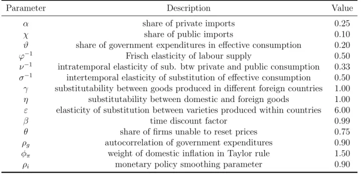
This subsection calibrates the SOE model aiming to study the e↵ects of fiscal policy in the Portuguese economy. When no estimates are available for EMU, US is used as a proxy for EMU. The calibration used in the simulation of the model is based on existing literature and is, as much as possible, empirically plausible. First of all, recall that the the intratemporal elasticity of substitution between private consumption and government expenditure (⌫ 1_{) and}

the households’ intertemporal elasticity of substitution ( 1_{) are the parameters defining the}

e↵ectiveness of fiscal stimuli. Therefore, an accurate estimation of these two parameters has a particular importance. Based in US data, the parameter ⌫ is estimated in Bouakez & Rebei (2007, p.971) where the authors suggest to calibrate ⌫ = 3.26 _{On the other hand, the}

param-eter 1 _{is estimated in Havr´anek et al. (2013) who collect more than two thousand estimates}

for the intertemporal elasticities of substitution worldwide. In the end, the authors suggest the value of 0.5 as the most plausible intertemporal elasticity of substitution which is the same to calibrate = 2. Taking into consideration these two estimates and Amano & Wirjanto (1998) classification concerning substitutability and complementarity, private consumption and government expenditures are modelled as complements. Moreover, the calibration is in line with empirical results of Section 1 which concludes that private consumption and government expenditure are, on average, complements. There is a complementarity relation because private consumption gives a positive response to most of government stimuli (even though its response does not always lead to a multiplier higher than one).

Another important aspect concerns the Frisch elasticity of labour supply (' 1_{) which is}

fixed at 0.5 based in Chetty et al. (2011). Equally important are the private and public propensities to import, ↵ and , respectively. These were calculated based in the Portuguese national accounts and Dias (2010, 2011) methodology.27 _{The shares of steady state private} rate whereas e! 1 then et= 0 which represent a fixed exchange rate regime.

26_{In Bouakez & Rebei (2007), the exponents of e↵ective consumption have an inverse structure relative to}

equation (2.2). For more details check Appendix B.2.

(41)

consumption and government expenditures in e↵ective consumption are calibrated according to the Portuguese economy, that is C_C_b = 0.80 and G_C_b = 0.20.28 _{The choice of the monetary}

policy parameter follows Taylor (1993) original calibration, i.e. ⇡ = 1.5.29 The remainder

of the values come from Gal´ı (2008, ch.7) open economy model.30 _{Table 1 summarizes the}

parameters choice used in the simulation exercise.

Table 1: Baseline Calibration

Parameter Description Value

↵ share of private imports 0.25 share of public imports 0.10 # share of government expenditures in e↵ective consumption 0.20 ' 1 _{Frisch elasticity of labour supply} _0.50

⌫ 1 _{intratemporal elasticity of sub. btw private and public consumption} _0.33 1 _{intertemporal elasticity of substitution of e↵ective consumption} _0.50

substitutability between goods produced in di↵erent foreign countries 1.00 ⌘ substitutability between domestic and foreign goods 1.00 " elasticity of substitution between varieties produced within countries 6.00 time discount factor 0.99 ✓ share of firms unable to reset prices 0.75 ⇢g autocorrelation of government expenditures 0.90 ⇡ weight of domestic inflation in Taylor rule 1.50

⇢i monetary policy smoothing parameter 0.90

28_{For additional details check the ”Economic Bulletin 10/2014” of the Bank of Portugal, page 7. These}

values are widely used in the literature see, among others, Christiano et al. (2011), Erceg & Lind´e (2014) and Bouakez & Rebei (2007).

29_{Du↵y & Xiao (2011) showed that Taylor original calibration produces determinacy in the several model}

specifications used. Moreover, the authors demonstrate that introducing policy smoothing, i.e., make the interest rate depend on its past values, increase the determinacy of the models.

(42)

3.2.1 Propensities to Import

The propensities to import of the main components of GDP have been measured in several recent articles, see, among others Dias (2010, 2011) and Cardoso et al. (2013) measuring the import contents of each aggregate demand component for the Portuguese economy. Aiming to find a plausible estimate for the share of imports of private consumption and government expenditure and also verify whether it changed over the years, Dias (2010) methodology was applied to the most recent data for the Portuguese economy, the year 2008. The methodology uses Input-Output matrices released by Instituto Nacional de Estat´ıstica (INE)31_{to measure}

the (direct and indirect) propensities to import of each aggregate demand component. The direct e↵ect accounts for the imports of inputs that each good or service use during the production process while the indirect e↵ect measures imports within national production used as intermediate consumption in other production processes.32 _{A summary of the results}

is presented below

Table 2: Percentage of Imports in each Final Demand Component in Portugal, 2008 Direct Indirect Total Households Consumption Expenditure 0,128 0,138 0,266 Government Consumption Expenditure 0,015 0,084 0,099 Gross Fixed Capital Expenditure 0,216 0,165 0,380

Exports 0,017 0,418 0,436 Total Final Demand 0,102 0,192 0,294

Source: Author’s calculations based in INE data and Dias (2010, 2011) methodology. Cardoso et al. (2013) using an identical but more aggregated methodology obtain identical results. Then, it may be assumed that the results above are corroborated. Nevertheless, in Corsetti et al. (2009) the government share of imports is calibrated to 6% highlighting the importance of government imports when analysing e↵ectiveness of fiscal policy.

(43)

3.3 Discussion and Results

This subsection quantitatively analyses the dynamics of an expansionary shock in domestic government expenditure under the baseline calibration. Figure 1 depicts the response of economic variables to a 1 standard deviation increase in the steady state level of govern-ment expenditure. The vertical axis of impulse response functions measure the percentage deviations of the variables from the respective steady state values while the horizontal axis measures quarters. Domestic inflation, CPI inflation and nominal interest rate are repre-sented as annualized quarterly rates. For the sake of comparison, the same government expenditure shock is analysed under pegged and flexible exchange rate. Figure 1 shows that both private consumption and output react positively to the simulation. With fixed exchange rate the reaction of output is more than one-for-one whereas in the flexible exchange regime output weakly responds to government expenditure. This leads to the conclusion that, in this model, fiscal policy is more e↵ective under a fixed exchange rate regime. Following the stimulus, the nominal exchange rate in the flexible exchange regime depreciates. The shock also makes the trade balance and terms of trade deteriorate. Nominal interest rate decreases and labour supply increases in both exchange regimes. However, real wage only responds positively in the fixed exchange regime. The conclusion that fiscal policy is more e↵ective in a fixed exchange regime is reinforced with an analysis of fiscal multipliers.

(44)

Figure 1: Impulse Response Functions for a Shock in Domestic Government Expenditure 0 2 4 6 8 10 12 14 16 18 20 0 1 2 Government Expenditure 0 2 4 6 8 10 12 14 16 18 20 0 2 4 Private Consumption 0 2 4 6 8 10 12 14 16 18 20 0 1 2 Output 0 2 4 6 8 10 12 14 16 18 20 −1 0 1 Output Gap 0 2 4 6 8 10 12 14 16 18 20 −4 −2 0 Terms of Trade 0 2 4 6 8 10 12 14 16 18 20 −1 −0.5 0 Trade Balance 0 2 4 6 8 10 12 14 16 18 20 −10 −5 0

Nominal Interest Rate

0 2 4 6 8 10 12 14 16 18 20 −5 0 5 CPI Inflation 0 2 4 6 8 10 12 14 16 18 20 0 1 2 Labour Supply 0 2 4 6 8 10 12 14 16 18 20 −4 −2 0

Nominal Exchange Rate

0 2 4 6 8 10 12 14 16 18 20 −2 0 2 Domestic Inflation 0 2 4 6 8 10 12 14 16 18 20 −5 0 5 Real Wage P E G D I T R

Note: Recall that DITR stands for domestic inflation Taylor rule and represents a flexible exchange rate regime. PEG denotes a fixed exchange regime.

(45)

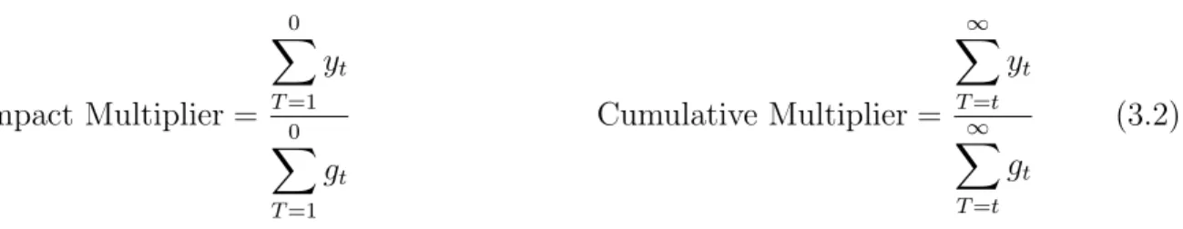
Impact Multiplier = 0 X T =1 yt 0 X T =1 gt Cumulative Multiplier = 1 X T =t yt 1 X T =t gt (3.2)

Impact multipliers measure the immediate response of output in percentage of government stimulus.33 _{In this model, the impact multiplier coincide with its peak. On the other hand,}

the cumulative multiplier also measures the response of output in percentage of government stimulus but it’s the long-run average. Table 3 easily illustrates the above conclusion. The impact multiplier in fixed exchange regime is about 1.6 while in the long-run it falls to 1. Much lower are the multipliers in the flexible exchange regime where fiscal multipliers achieve 0.2 on impact and 0.7 cumulative.

Table 3: Fiscal Multipliers Fixed Flexible Impact 1.6 0.2 Cumulative 1.0 0.7

33_{Note that the specification of fiscal multipliers used in this model is di↵erent than the traditional one}

(where it is usually a ratio between variables measured in levels). In this case, the fiscal multiplier is a ratio of two variables measured in percentage deviations from respective steady state. If the initial values are not

(46)

To simulate a government expenditure shock in EMU and have a better understanding of its consequences, a more comprehensive analysis of fixed exchange regime is made. The fixed exchange regime does not allow the currency to depreciate and consequently does not force private consumption to adjust to higher foreign prices (when converted to domestic currency). This makes the response of aggregate demand much stronger than it would be in the case of a flexible exchange rate. In flexible exchange regimes, the depreciation of the exchange rate establishes higher foreign prices when converted to domestic currency and mitigates a wave of imports. In the context of fixed exchange regime, represented in Figure 1, the trade balance is dampened with the increase in both private and public consumption. Once government also purchases abroad the stimulus weakens net exports. Take into account that the terms of trade, influenced by the exchange rate regime, also foster this unfavourable behaviour of the net exports.

Another important but expected finding concerns the labour supply which is found to increase and partly o↵set the negative wealth e↵ect induced by the fiscal shock. The increase in labour supply is understandable in the light that households want to smooth their con-sumption and to do so need to work more. Remember that the fiscal stimulus is financed through a tax over households current income. Certainly, the impulse response function of labour supply is much pronounced due to the complementarity because households will want to consume public and private goods together. On the other hand, the short-term nominal interest decreases and real wage increases which will tend to further amplify the positive reaction of private consumption. Households intertemporally substitute future consumption for current consumption decreasing their savings due to its low return. In summary is pos-sible to conclude that non-separability and complementarity between private consumption and government expenditure induce a positive response of private consumption to a govern-ment expenditure shock. Private consumption reaction is strengthened by: (i) the degree of complementarity (⌫ ), (ii) the fixed exchange regime, (iii) the increase in working hours and (iv) the decrease in the nominal interest rate.

(47)

Finally, notice that all world variables are invariant to any domestic shock because the home economy has an infinitesimally small size in comparison to the world economy. However, a shock of the world economy may a↵ect the domestic economy through cross-border spillover e↵ects.

One of the assumptions of this model is the Uncovered Interest Parity (UIP) defining the domestic economy interest rate as a function of world interest rate and expected change in the nominal exchange rate.34 _{Naturally, in a fixed exchange regime, nominal interest rate}

should not vary. However, non-separable preferences ( 6= ⌫ and # > 0) break the UIP condition and thus nominal interest rate varies in response to a fiscal stimulus. From here a conclusion emerges, an exogenous government expenditure shock in a model with non-separable preferences has a profound impact in the households optimization problem such that the behaviour of nominal interest rate is distorted.35 _{Appendix A.8 shows how UIP}

does not hold. In this model, the relation between domestic and foreign interest rates is represented by:

it = i⇤t + Et{ et+1} 2 ( ⌫) Et{ bct+1} Et bc⇤t+1 . (3.3)

From this equation a conclusion emerges, UIP does not hold as long as there is non-separability, i.e. 6= ⌫. Next this conclusion is illustrated numerically.

34_{The UIP is represented as follows i}

Fiscal multipliers and non-separable preferences in a small open economy model