Thumb Consumers
Rodrigo M. Pereira
∗
Contents: 1. Introduction; 2. Rule of Thumb Behavior and Habits in a Small Open Economy; 3. Estimation Strategy; 4. Empirical Results; 5. Conclusion; A. Appendix 1; B. Appendix 2.
Keywords: Rule of Thumb; Consumption; Current Account; Habit Formation.
JEL Code: C22, E21, F32.
In this paper the idea of rule of thumb consumption, in which some households do not behave according to the Permanent Income Hypothesis, is applied to a small open economy framework. A model of current account with rule of thumb individuals and habit formation is presented and estimated for five different countries. Two parameters of the model are of particular interest: the share of domestic income that accrues to rule of thumb individuals and the coefficient of habit forma-tion. Using current account data, the results obtained here support the view that rule of thumb behavior plays a major role in the economy. Moreover, the estimated habit formation coefficients are mostly small and nonsignificant.
Nesse artigo a ideia do consumo regra de bolso, em que algumas famílias não se comportam de acordo com a Hipótese da Renda Permanente, é apli-cada a uma estrutura de uma pequena economia aberta. Apresentamos um modelo de conta corrente com indivíduos se comportando pela regra de bolso e com formação de hábitos. O modelo é estimado separadamente com dados de cinco países. Estamos particularmente interessados em dois parâmetros do modelo: a razão da renda agregada doméstica aferida por indivíduos regra de bolso, e o coeficiente de formação de hábitos. Utilizando dados de conta corrente, os resultados obtidos sugerem que o comporta-mento regra de bolso tem um papel importante na economia. Ademais, os coeficientes de formação de hábitos estimados são em geral pequenos e não-significantes.
1. INTRODUCTION
The analysis of current account dynamics has experienced substantial developments in the last two decades. After the early works of Sachs (1981) and Svenson and Razin (1983), the Mundell-Fleming treat-ment of the current account was quickly replaced by dynamic intertemporal models in the literature. This new generation of models relied on partial equilibrium frameworks of a small economy, which allowed consumption and production decisions to be made independently of each other. Underneath this important feature was the idea that the economy to be modeled is so small that its decisions does not affect world interest rates. By assuming that this small economy is inhabited by identical individ-uals, it was possible to theoretically tie the current account behavior of a country to the consumption behavior of its representative individual, with national output (net of government expenditures and private investment) playing the role of labor income and current account playing the role of savings. It soon became apparent that a vast area of potential research was opened with this linkage between modern consumption theory and the current account.
In principle, current account models are able to inherit most of the leading ideas underlying con-sumption theory. The transposition of these ideas to an open economy context has taken place quite often in the literature. Habit formation, for example, is an important insight in consumption theory that was explored by Constantinides (1990), among others. Subsequently, habit-forming consumers were introduced in an open economy model by Obstfeld (1992), and more recently by Ikeda and Gombi (1998). Another example of the tight link between the consumption and current account theories comes from the study of Campbell (1987), who develops a new econometric approach to test the permanent income hypothesis. Campbell argues that if consumers really smooth consumption, saving for the bad times and overconsuming when current income is lower than permanent income, then declines in la-bor earnings should be accurately predicted by savings. The predictive power of savings is then tested using an econometric method that conveniently tackles nonstationarity issues. Sheffrin and Woo (1990) then apply the technique developed by Campbell to a current account model. They test whether current account is a good predictor of fluctuations in the domestic net output (defined as GDP minus the sum of investment and government expenditures). They perform the tests using data of four small economies, concluding that the predicted and actual data are reasonably close in two of these economies.
In this paper I follow this stream of borrowing ideas from the consumption literature and applying them into a model of current account. One important insight developed for consumption models that still remains unexplored in an open economy context is the rule of thumb behavior. Initially idealized by Campbell and Mankiw (1989) as a theoretical answer for the mismatch between Hall (1978) famous result that consumption follows a random walk, and empirical evidence suggesting that income helps to predict consumption, the rule of thumb was a simple idea. Basically, it states that only a fraction
of the disposable income in the economy, say,1−λ, accrues to consumers that behave according to
the permanent income hypothesis. Another fractionλgoes to individuals that simply spend all their
current income. The debate about the quantitative importance of the rule of thumb behavior is far from being settled. Some studies suggest that rule of thumb consumers respond for a large portion of the disposable income. Campbell and Mankiw (1989, 1990) find that about 50% of the disposable income goes to rule of thumb consumers. Cushing (1992) and Weber (2002) investigate whether current income consumption is still relevant when time non-separability is introduced in the consumption function. They obtain opposed results. Cushing finds that current income consumption is important, arguing that such behavior is mainly related to the household’s lack of credit. Weber shows that if time
non-separability is not modeled, then the estimates of λwill be upward biased. This author uses the
generalized method of moments to estimateλunder different functional forms for the utility function.
He finds values forλthat are either small or negative, and statistically nonsignificant.
of riskless foreign bond. The only departure here is that instead of a single representative consumer, there are two types of consumers: the rule of thumbs and the permanent incomes. Because rule of thumb households do not borrow nor lend money, the amount of foreign assets in the small economy corresponds to the amount of foreign assets held by permanent income households. It turns out that the standard current account identity can be used in the constraint of the representative permanent income consumer’s maximization problem, generating the core equation of the model. Another impor-tant point is that it is assumed that permanent income individuals are subject to habit formation, in the sense that their instantaneous utility function relates their utility to a linear combination of their current consumption and the lagged value of average consumption. The resulting framework is, to the best of my knowledge, the first to mingle the literatures on current account determination and the rule of thumb consumption. Moreover, this is the first study that estimates the rule of thumb parameter using current account data.
Empirically, the goal of the paper is twofold. On one hand, the paper addresses an issue related to the consumption literature, which is the estimation of the rule of thumb parameter. So, essentially the analysis pursuits an answer to the following question. Under the framework of a small open economy, does the empirical evidence suggests a high and significant share of rule of thumb behavior in the
economy? Or, does the use of current account data ratify the findings of Weber (2002) thatλis small
and mostly nonsignificant when social habits are taken into account? The model is estimated using instrumental variables techniques, and then the robustness of these estimates is assessed through tests based on some cointegrating relations that should take place according to the theoretical structure. On the other hand, the paper also goes through an exercise that is related to the current account literature. In the same fashion as in Sheffrin and Woo (1990), the idea is to analyze how well the model performs in describing the current account dynamic behavior in a small open economy. Is the rule of thumb feature helpful in enhancing the predictive power of the model? The comparison of the actual and fitted current account series is used as an indication of the model’s accuracy.
The rest of the paper is organized as follows. Section 2 develops a model of current account with rule of thumb consumers. Section 3 presents the econometric procedures used to implement and test the model empirically. These procedures rely essentially on instrumental variables estimations and cointegration tests. In section 4 the tests are performed to ten developed and developing economies. It turns out that among these ten countries, only five have data that satisfy certain stationarity conditions that are required to hold for the model to be tested. The procedures are then implemented for these five economies, namely, Australia, Italy, Spain, South Africa and Turkey. Section 5 concludes the paper.
2. RULE OF THUMB BEHAVIOR AND HABITS IN A SMALL OPEN ECONOMY
In this section I present a model of current account dynamics that incorporates the ideas of rule of thumb consumption and habit formation. The model describes a small economy in the sense that the consumption, investment, and production decisions taken domestically do not affect the world interest rates. Also, it is assumed that individuals live forever, and that only a riskless asset is traded inter-nationally. Some households in this economy behave according to the permanent income hypothesis, changing current consumption only when a change in permanent income is perceived. The remaining households, however, completely spend their current income at each point in time.
Habit formation is typically modeled in the literature through some type of time non-separability in the instantaneous utility function. By that means, the utility derived today depends not only on today’s consumption, but also on the consumption in past periods. Here, habits are represented by the average, instead of the individual past consumption.
That is not the case with average consumption. The household believes that he is small enough such
that his consumption decision does not affect the average consumption in the economy.1
The theoretical framework is essentially centered in the maximization problem of the permanent income consumers. The main insight of the model is that the intertemporal budget constraint of per-manent income consumers can be expressed using the current account identity. This comes from the assumption that the rule of thumbs always spend their current income, and consequently are always in a net position of zero debt in terms of the international bond.
2.1. Government
The government in this small economy taxes income at the constant rate ofτ, collectingτ Ytin
taxes and spendsGt in provisions of goods and services to the households. It is assumed that the
government runs a balanced budget at each point in time, i.e.,τ Yt =Gt,∀t. Since individuals live
forever in this framework, Ricardian equivalence holds. Consequently, the balance budget assumption does not change households’ reaction to changes in the government expenditure level. In other words, households’ consumption path is the same, no matter if taxes are raised today or in the future. Also, I assume that government expenditures are perceived as a waste by the individuals, who do not benefit
fromGtin terms of utility gains.
Because of the separability between consumption and production decisions in this theoretical frame-work, the production side of the economy does not need to be explicitly structured in order for the model to generate a tractable current account equation. However, it is worth mentioning that the la-bor supply decisions are completely bypassed in this analysis. It is implicitly assumed that individuals supply their labor inelastically, and that labor time does not pose any kind of disutility in households preferences.
2.2. Consumption
Consider a small economy inhabited by two types of infinite-lived consumers. The first type is the consumer that behaves according to the permanent income hypothesis, smoothing consumption through his lifetime. The second type is the rule of thumb consumer, that just spends his entire current
disposable income at each point in time. LetYrtandYptbe the incomes of the rule of thumb group and
the permanent income group, respectively. Ifλis the fraction of the domestic income that goes to rule
of thumb consumers, thenYrt =λYt, andYpt = (1−λ)Yt., whereYtis the total domestic income.
Also, letCrtandCptbe the consumption of the rule of thumb and the permanent income consumers,
respectively. Total consumption is therefore
Ct=Crt+Cpt= (1−τ)λYt+Cpt (1)
It is assumed that there is a single asset in the world that can be transactioned internationally
yielding the world interest rate ofr. Following Weber (2002), I assume that the permanent income
consumers have social habits in such a way that current utility depends not only on the current individ-ual consumption, but also on the lagged average consumption of all households. Thus, the permanent income household maximizes his expected lifetime utility given by
V =Eo
∞ X
i=0
βiU(C
pt+i−θCt−1+i), C−1given (2)
1A natural issue here is that by being a representative consumer, his decision indeed affects the average consumption (since
where the termθstands for the degree of social habit in the utility function, andβis the time discount factor. It is implicitly assumed that individuals do not assign utility to leisure. The utility maximization of the representative agent has the following budget constraint
−Dt+1+i+Dt+i = (1−τ)Ypt+i−rDt+i−Cpt+i−Ipt+i (3)
whereDtrepresents the individual’s debt position in terms of the international asset, andIptis the
amount of resources invested in the production sector. Let the period utility function be represented by a linear-quadratic functional form given by
U(Cpt+i−θCt−1+i) = (Cpt+i−θCt−1+i)−
h
2(Cpt+i−θCt−1+i)2 (4)
withh >0. Linear-quadratic specifications are very convenient, and in many cases are the only way
to obtain a closed-form solution. They are also widely used in the current account literature (see, for example, Glick and Rogoff (1995), Frenkel and Razin (1996). Indeed, the linear-quadratic form in (4) is
a generalization of the form used by Glick and Rogoff (1995), in which habit formation is allowed.2
Assuming thatβ(1 +r) = 1, in order to rule out consumption tilting, we have the following first order
condition3
EtCpt+1−Cpt=θ(Ct−Ct−1) (5)
Expression (5) states that the change in average consumption helps to predict the consumption of the representative permanent income household. In this framework, Hall’s (1978) random walk result
applies only when habit formation does not exist(θ = 0). Letηt+1 = Cpt+1−EtCpt+1denote the
forecast error of permanent income consumption. Then, expression (5) can be rewritten as
∆Cpt+1=θ∆Ct+ηt+1 (6)
The possibility of borrowing indefinitely in a kind ofPonzischeme should be ruled out. Thus, the
optimality equation (5) holds subject to the following transversality condition
lim
T→∞
1 1 +r
T
Dt+T+1= 0 (7)
Since rule of thumb individuals do not save, all the investment in the economy is done by the
permanent income consumers, implying thatIpt+i =It+i.With the assumption that the government
runs a balanced budget, it is straightforward to see that the left-hand side of expression (3) denotes the country’s current account, given by
CAt+i=−Dt+1+i+Dt+i=Yt+i−rDt+i−Ct+i−It+i−Gt+i (8)
Substituting for the definition of total consumption (1), and rearranging terms, we have
CAt+i = (1−λ)(Yt+i−Gt+i)−rDt+i−Cpt+i−It+i (9)
Taking first differences fori= 0, and substituting (6) into the resulting expression, one obtains
2Ifθ= 0, then expression (4) in the text becomes exactly the instant utility function used by Glick and Rogoff (1995). 3If individual past consumption were used to model habits, than second order lagsC
t−2would show up in the first order
condition. However, as mentioned earlier, we use average past consumption, that could be treated as a constant to our individual consumer. Hence, the first order condition with the debt as the choice variable is given by
1−h2[Cpt−θCt−1] 2 +βEt n
[−1(1 +r)]−h22 [Cpt+1−θCt] [−(1 +r)]
CAt+1= (1 +r)CAt+ (1−λ)(∆Yt+1−∆Gt+1)−θ∆Ct−∆It+1+εt+1 (10)
whereεt=−ηt. Expression (9) relates the current account with its lagged value and first-differences
of aggregate output, government expenditures, aggregate consumption, and aggregate investment. If all these variables are stationary in first differences and the current account is stationary in levels, this equation can be estimated using conventional econometric techniques, providing consistent estimates
of the share of rule of thumb consumers in the economy,λ, and the parameter for the habit formation
degree,θ.
An important issue in the estimation of (10) is that the residualεtis related to the forecast error
of the permanent income consumption. It is quite sensible to suspect that this error might not be orthogonal to the variation in income. The intuition is simple. Suppose an unexpected increase in the
current income fromttot+ 1. The higher the increase in current income, the more it spills over the
permanent income, the higher is the raise in consumption int+ 1, and the larger is the forecast error
of permanent income consumption int. Consequently, the error term in (10) would be correlated with
one of the regressors, and OLS estimation would not yield consistent estimates of the parameters. We rely on instrumental variables (IV) techniques to fix this problem.
Since the influential work of Nelson and Plosser (1982), there has been a great deal of evidence suggesting that aggregate output, consumption, investment and government expenditures typically contain stochastic trends. In the next two propositions it is assumed that each of these variables have one unit root. Henceforth I(1) stands for the presence of one unit root (or integration of order one), and I(0) stands for stationarity (or integration of order zero). Proposition 2 uses the econometric concept of cointegration, in which a set of variables with the same order of integration, can be combined in one (or eventually more than one) particular linear combination that has a lower order of integration.
Proposition 2.1. If aggregate output, Yt, consumption,Ct, investment,It and government expenditures,
Gt,are I(1), then the current account,CAt, is I(0).
Proof. : (see Appendix)
Proposition2.2. IfYt,Ct,It,Gt, and foreign debt,Dt, are I(1), then either: (i)CtandYtare cointegrated,
with cointegration vector(1,−(1−τ)λ), the aggregate consumption of permanent income households,
Cpt, is I(0), andYt,Gt,It, andDt, cointegrate with cointegration vector(1−λ,λ−1,−1,−r); or (ii)
CtandYtare not cointegrated,Cpt,is I(1), andYt,Gt,Cpt,It,andDt, cointegrate with cointegration vector
(1−λ,λ−1,−1,−1,−r);
Proposition 2 is a straightforward step ahead of proposition 1, and does not require a formal proof.
The definition ofCptin (1), states that it is a linear combination of two arguably I(1) variables,Ytand
Ct Then, ifCpt, is I(0) part (i) of proposition 2 applies. If Cpt, is I(1), however, thenYtandCtdo not
cointegrate. In this case, the current account, which should be stationary according to proposition 1, is a linear combination of I(1) variables, as can be seen in expression (9). Then, these I(1) variables should necessarily cointegrate, and part (ii) of proposition 2 holds.
In the next section, I present the strategy used to tackle the main empirical issues addressed by the paper.
3. ESTIMATION STRATEGY
The estimation of the current account equation (10) involves two different issues. The first one,
which is related to the consumption literature, is the estimation of the rule of thumb parameter λ.
λis small and mostly nonsignificant be replicated here, using current account data? The OLS and IV estimation of (10) should be another piece of evidence in the debate about whether or not rule of thumb consumption is a phenomenon that really matters.
The second issue is related to the current account literature. By estimating equation (10), it is possible to access the quality of the model in terms of replicating the current account dynamic behavior in small open economies. In line with the works of Sheffrin and Woo (1990) and Ghosh (1995), it is possible here to compare the actual current account time series with the series predicted by the model. The similarity between these two series, along with the coefficient of determination R2, gives us an idea of how well the model performs.
Even though the estimation of equation (10) through OLS and IV is quite straightforward, there are other interesting procedures that can be done. Specifically, it is possible to use the knowledge of propo-sition 2 about the cointegrating relations to evaluate the robustness of these OLS and IV estimations. Thus, the first step is to rearrange the terms in (10)
CAt+1−(1 +r)CAt+ ∆It+1= (1−λ)(∆Yt+1−∆Gt+1)−θ∆Ct+εt+1 (11)
The estimation of the interest rateras a coefficient can be particularly troublesome.4Hence, instead
of trying to estimater, I follow the practice of presetting values for it. That yields a time series for the
left-hand side of (11). So, initially I estimate equation (11) using IV techniques. The chosen instruments are lagged values of the explanatory variables and of the current account. Just as a reference, I also perform OLS estimation on (11).
Proposition 2 states that there must exist a number of cointegrating relations between certain vari-ables of the model, and that the corresponding cointegration vectors invariably involve the parameter
λ. So, by performing cointegration tests with these variables, it is possible to obtain a super consistent
estimate ofλ. How close this estimate is from the original IV estimation should then be a good proxy
of how robust the IV estimate is.
One problem with this approach is that the consumption of permanent income households,Cpt, is
not observable. To circumvent this issue, I use a proxy time series ofCptbased on the relation given by
(1), and IV estimates ofλand OLS estimates ofτ. So, the cointegration tests are performed withCpt
proxied byCˆpt =Ct−(1−ˆτ)ˆλYt, whereˆλandτˆare the IV estimates ofλand OLS estimates ofτ,
respectively. The estimate ofτis based on the government balanced budget relation. It is possible to
obtain a consistent estimate ofτthrough the OLS estimation of
∆Gt=τ∆Yt+υt (12)
whereυtis an i.i.d. residual. The next step is to check ifCtandYtcointegrate. If yes, the estimated
cointegration vector can be compared with the vector(1,−(1−τˆ)ˆλ)constructed with IV and OLS
es-timations. How close they are should give a good indication of the robustness of the original estimates.
IfCtandYtdo not cointegrate then we should move to the second part of Proposition 2, and check if
Yt,Gt,Cpt,It,andDtcointegrate. If they do, then the robustness can be assessed by comparing the
estimate of1−λembodied in the cointegration relationship with the previous IV and OLS estimates of
1−λ. The popular Johansen method is used to test for the existence of cointegration.
4. EMPIRICAL RESULTS
When the current account and the explanatory variables in the right-hand side of (10) are stationary,
then IV estimation provides consistent estimates of the parametersλand θ. However, if any of the
4It worth noting that the interest rate here plays the role of the intertemporal discount factor in the typical linear-quadratic
terms in (10) has unit roots, then the use of instrumental variables involves the classic issue of spurious regression. So, before addressing the estimation of (10), I’ll test for the stationary of the variables in equation (10).
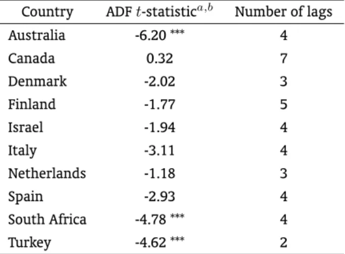
Initially, I perform Augmented Dickey-Fuller tests for the presence of unit roots in the current ac-count data of 10 ac-countries. The tests use quarterly data from IMF’s International Financial Statistics data set (see Appendix 2 for more details on how the data is assembled for the estimation). The results for the 10 countries are presented in Table B-1. Interestingly, the table suggests that the series of cur-rent account does have unit roots in several cases, in contradiction with the theoretical predictions. For three countries, Australia, South Africa and Turkey, the null hypothesis of a unit root is ovewhelmingly rejected. For all the others, however, the null is accepted at the conventional levels of significance. The tests are performed with a constant and a trend as deterministic regressors, but the results are quite robust to other specifications without the trend and without the constant and the trend (the only
exception being Italy and Spain, whose ADFt-statistics become significant at 5%).
Given that the proposed method of estimating equation (10) requires current account stationarity, the countries that exhibit unit roots will be ruled out . So, the model will be tested for Australia, South Africa, Turkey, Italy and Spain. Even though Table B-1 does not report significance at the usual levels for Italy and Spain, it is worth mentioning that p-values are slightly higher than 10%. Also, the well known lack of power of ADF tests to reject the null and the fact that the null is rejected when the test is performed without deterministic trend and constant, suggest that the current account in these two countries could very well be stationary.
Table B-2 presents the results of ADF tests for the six key variables of the model, in levels and in first differences, for the five aforementioned countries. For convenience, the current account results in Table B-1 are repeated in Table B-2. The debt in foreign currency, aggregate consumption, government expenditures, aggregate investment and GDP seem to have a unit root in almost all the cases. The
only exception being Turkey, whose ADFt-statistic is high enough to reject the null at 10% in the case
of aggregate consumption and GDP. For the data in first differences, however, the null of a unit root is rejected at 1% of significance in almost all the cases, suggesting that the debt in foreign currency, aggregate consumption, government expenditures, aggregate investment and GDP do not have two unit roots. Again, the tests are performed with a trend and a constant, but the results without the trend and without the trend and the constant are quite similar. So, based on the evidence of Table B-1, I will assume that the current account is stationary, and that the debt, consumption, government expenditures, investment and GDP are I (1) in the five countries.
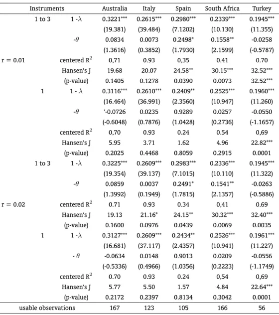
The results of the OLS and IV estimation for the current account equation (10) are presented in Table B-3 and Table B-4, respectively. The estimates obtained with IV’s are quite close to the ones obtained with OLS. The instruments are lagged values of the current account and of the exogenous variables. The tests are performed with two different sets of instruments: lags from 1 to 3, and the first lag. The results in Table B-4 are not very sensitive with respect to the choice of lags (perhaps, with the exception of Spain). The regressions are performed with interest rates preset at 1% and 2% per quarter (which correspond approximately to 4.06% and 8.24% per year). Changing the interest rate has very small effects on the estimates, as can be seen in tables B-3 and B-4.
The use of lagged values of the key macroeconomic variables included in the model as instruments is a standard procedure in the literature. The idea is to avoid the endogeneity of the intruments. In our setup we have more instruments than endogenous regressors, which means we can perform Hansen’s J test for overidentifying restrictions. The test basically runs the residuals of the second stage regression
on the set of instruments. The test statistics has aχ2
(m−k)distribution where m is the number of
The first stage regression in our IV estimation is presented in Table B-5. We have the results of OLS
regression of the variable that is being instrumented,∆Yt−∆Gt, on the two different sets of
instru-ments. Past consumption seems to be a particulartly important instrument for all the five countries. The table reports the F statistics for these first stage regressions, which in this context serves the pur-pose of testing for weak instruments. We obtain very high F statistics, which suggests that we don’t have problems of weak instruments.
With the two levels of interest rate, the share of national income that accrues to permanent income consumers is surprisingly low, and in all cases the estimates are highly significant. Both the OLS and the IV estimations suggest that something around 70% to 80% of the disposable income goes to the
rule of thumb households (i.e.,1−λlies roughly between 0.3 and 0.2). These values are considerably
higher than what has been found previously in the literature,5providing strong support for the view
that rule of thumb behavior is an important phenomenon in the economy. Moreover, these findings are not subjected to the criticism of Weber (2002), who shows that estimates of the importance of rule of thumb behavior that do not account for habit formation are invariably upward biased. Indeed, our results suggest that, in an open economy, the rule of thumb behavior is still relevant even when habit formation is considered. Moreover, Tables B-3 and B-4 reveal that if there is something empirically unimportant in the model, it is the coefficient of habit formation, and not the rule of thumb behavior.
The estimates of the parameter of habit formationθreported in Table B-3 and Table B-4 are very small
and, for most of the countries, not significant at the conventional levels (the only exception being Spain, whose estimate is significant at the 10% level in Table B-3 and in some regressions of Table B-4, and South Africa, whose estimates are significant at the 5% in half of its regressions in Table B-4).
The estimates of the taxation parameterτ are presented in Table B-6. They are obtained through
OLS estimation of equation (12). The estimates seem reasonable, and are significant at the 1% level
for all the five countries. The value ofτfor Turkey is remarkably small as compared to the other four
countries analyzed. Once the estimates ofτ andλare calculated, it is possible to construct a proxy
series for the permanent income consumers,Cpt.
Initially we have to test if the first part of Proposition 2 applies to any of the five countries, i.e., if total aggregate consumption and aggregate income cointegrate. The simplest way to do that is to use the so called Engle-Granger methodology and check if the given linear relation between these I(1)
variables is stationary. 6 The results of the ADF tests on the proxies forCptare presented in Table B-7.
To generateCptI use the estimates ofτin Table B-6 and I arbitrarily choose the IV estimates ofλwith
r= 0.01and with lags from one to three of the instruments (first line of Table B-4). For Australia, the
ADF test suggests that the consumption of permanent income individuals is stationary, and therefore that aggregate consumption and income cointegrate. The null of a unit root is rejected even at the 1% level. For the other countries the null hypothesis of a unit root cannot be rejected at the usual levels of significance. So, the results suggest that for these countries the consumption of permanent income households is non-stationary, and consequently, total aggregate consumption and aggregate income do
not cointegrate with the cointegration vector(1,−(1−τ)λ). The tests were performed with a trend
and an intercept, but other specifications without the trend and without the trend and the intercept yield similar results (with the only difference that in these cases the null of a unit root in Australia is rejected only at the 10% level).
5Weber (2002) classifies the previous studies about rule of thumb consumers in two main groups. Authors like Campbell and
Mankiw (1989, 1990) and Cushing (1992) obtain large estimates of the rule of thumb behavior in the economy (something between 30% and 60% of the disposable income). A second group argues that rule of thumbs are not important quantitatively, reporting estimates ranging between 15% and 23%.
6The Engel-Granger method typically estimates (through OLS) a linear combination between the variables tha are being tested
for cointegration. Then the stationarity test is performed on the residual of this regression. A well known drawback of the method is that the results might differ according to the variable that goes in the left-hand side of the regression equation. In this paper, however, we have a very good clue of the linear relation betweenCtandYt(given by equation (1)), and thus the
To reinforce these conclusions I also perform the Johansen test for the cointegration rank. The popular Johansen’s methodology is based on the idea that in an error correction model, the rank of the matrix of equilibrium vectors has to be equal to the number of cointegration relationships. Since that rank also refers to the number of non-zero eigenvectors, it suffices to test for how many eigenvectors
are significantly different from zero.
The results of the Johansen tests for cointegration between aggregate consumption and income are presented in Table B-8. The lag length of the error correction model is chosen by applying the multivariate generalization of the Akaike Information Criterion (AIC) to the VAR portion of the model. I arbitrarily imposed a maximum acceptable number of 8 lags (2 years). So, the lag length in the test is the one that provides the least AIC value in specifications that include from 0 to 8 lags. For all the
five countries the choice based on the AIC criterion is 8 lags.7 Since the Johansen procedure is known
to be quite sensitive to the choice of lags, I also do the test with 4 lags. The results presented here are for tests performed without a drift or intercept, but similar results are obtained with these other specifications. Overall, Table B-8 confirms that there is no cointegration between consumption and income in Italy, Spain, South Africa and Turkey. Australia is again the only exception. The test provides a mild evidence of the existence of cointegration, with one positive eigenvalue at the 10% level of significance. However, at the 95% and 99% levels, the test cannot reject the null that the highest eigenvalue is equal to zero. For the other four countries the test provides overwhelming evidence that consumption and income do not cointegrate.
The cointegration vector of consumption and income in Australia estimated with the Johansen
method (using 8 lags in the error correction structure) is given by(1,−0.593), where the consumption
coefficient is normalized to one. The income coefficient is remarkably close to the OLS and IV estimates
ofτ andλ. Considering again the estimate ofτin Table B-6 and the estimate ofλin the first line of
Table B-4, we have−(1−ˆτ)ˆλ = −(1−0.1596)(0.6779) = −0.5697. The proximity of these two
estimates provides a strong indication of the robustness of the IV estimates ofλfor Australia.8
To verify for the robustness of the estimates of the other four countries, we should move to the
second part of Proposition 2, and perform the cointegration tests involving Yt,Gt,Cpt,Itand Dt.
The Johansen test is performed to check for the existence of cointegration relations. The choice of the optimal lag length in the cointegration tests is done through the Schwartz Bayesian Criterion (SBC). The Criterion is applied to the VAR portion of the error correction model, and again, I imposed a maximum number of lags of 8. Table B-9 presents the results for models without a drift vector and without intercepts in the cointegrating relations (the test with a drift vector and the test with an intercept in the cointegration vector were also performed, but did not present different results). For Italy and Turkey, the test suggests that only the highest eigenvalue is significantly different from zero, and consequently the matrix that multiplies the vector in levels in the standard error correction model has rank 1, and only one cointegration vector exists for these variables. For Spain, the Johansen test suggests the existence of two cointegrating relationships, and for South Africa the test has conflicting results, with
theλ-max statistic suggesting two and theλ-trace statistic suggesting one cointegration vector.
According to Proposition 2, the cointegrating vectors should have the coefficient ofDt equal to
0.01, the coefficients ofCptandItboth equal to one, and the coefficients ofYtshould be the negative
ofGt’s coefficient. So, instead of relying on unrestricted vectors that most likely would not have values
close what is stated by Proposition 2, I impose three restrictions on the vectors. The first one is that
7This oddity possibly comes from the fact that the system has only two variables. That means that an additional lag does
not increase dramatically the number of parameters to be estimated, which is the term that is traded-off in the AIC criterion against a reduction in the variance/covariance matrix of the residuals.
8Following the suggestion of an anonymous referee, I use the second part of proposition 2(i), in which I test for the cointegration
ofYt,Gt,It, andDtwith Australian data. With eight lags in the model we obtain only one eigenvalue significantly different
from zero. We then estimated the cointegrating vector with two restrictions, namely, equal coefficients with opposed signs for
YtandGt; and the coefficient ofDtbeing 1/100 of the one fromIt. We obtain the following vector: (-0.01, 1, 0.260, and
the coefficients ofCptandItare equal (by choosing one of these two variables to normalize the vector,
we get the desired unitary coefficients); the second one is that the coefficient ofDtis1/100of the
coefficient ofCpt; and the third one is that the coefficients ofYtandGtare equal, with opposite signs.
With these restrictions it is possible to pin down some features of the cointegrating vector that are not
the focus of the paper, and concentrate on the estimation of the parameterλ.
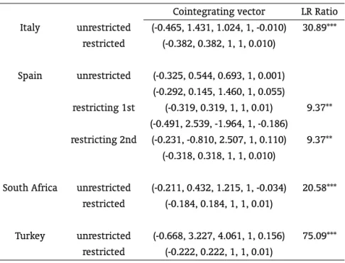
The restricted and unrestricted estimates of the cointegrating vectors are presented in Table B-10. The table also presents the Likelihood Ratio (LR) tests for the the validity of the restrictions. With 3 restrictions the statistic has a qui-square distribution with 3 degrees of freedom. The null hypothesis that the likelihood is not significantly changed when the restricitions are applied is rejected at the 5% level for all the four countries. Yet, this result should not be a problem. First, because we are imposing ad hoc restrictions on the interest rate, a regular practice in the literature. As we set it at 1% per quarter, we introduce a considerable departure from the unreasonable values found within the unrestricted vector, such as a quarterly rate of -3.4% in Soputh Africa or 15.6% in Turkey (see Table B-10). Second, because this is not our core estimation, which is based on IV techniques, but rather only a method to verify the robustness of our previous results.
The restricted estimates of the cointegrating vector(Yt,Gt,Cpt,It,Dt) for Italy and Turkey are,
respectively(−0.382,0.382,1.00,1.00,0.01)and(−0.222,0.222,1.00,1.00,0.01). For Turkey, the super
consistent estimate of1−λ = 0.222 is relatively close to the values estimated with instrumental
variables (which are roughly0.2). Nevertheless, for Italy the values are not quite close (0.382against,
for example, 0.2615in the first line of Table B-4). In the case of Spain, I allow for the estimation of
two cointegrating vectors, applying the set of three restrictions initially to the first vector (with the second one unrestricted), and then to the second vector (with the first one unrestricted). The results are presented below
1st vector restricted 2nd vector restricted
(−0.319,0.319,1.00,1.00,0.01) (0.312,−1.468,1.00,−0.674,0.104) (0.165,−1.052,1.00,−0.283,0.082) (−0.318,0.318,1.00,1.00,0.01)
The estimates of1−λ= 0.319and= 0.318are very similar to most of the estimates previously
obtained with OLS and IV techniques, that lie around0.3. So, the OLS/IV and the Johansen estimates
differ only by an amount around0.02in the case of Spain. The restricted estimate of one cointegrating
vector for South Africa is (−0.184,0.184,1.00,1.00,0.01). The estimate considering the existence of
two cointegrating vectors was also performed, but the estimate of1−λremained exactly the value
of0.184that was found with one cointegration vector, no matter if the restrictions were posed in the
first or second vector. This value is reasonably close to the OLS/IV estimates for South Africa, which are values between 0.23 and 0.28.
Summarizing, the estimates for Australia, Turkey and Spain seem to be very robust. The values that were found with OLS and IV techniques are very close to the values obtained with the Johansen method of testing for cointegration relations. For Italy and South Africa the values obtained with the two econometric procedures are still reasonably similar. They all suggest, however, a high and significant role for the rule of thumb behavior in the economy.
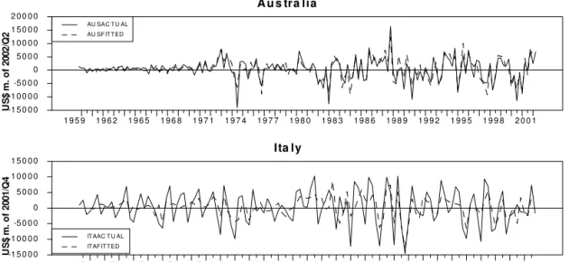
Another issue of interest is to check if the theoretical model of section 2 does a god job in describing
the current account dynamics. The centeredR2statistic gives an idea about this. In almost all OLS
and IV estimations the centeredR2’s are quite high, as reported in Tables B-3 and 4. An interesting
exercise is to plot the fitted and actual series of the current account in a graph. Here, the limitation of this exercise is that the dependent variable in the OLS and IV estimations is not the current account,
but rather the termCAt+1−(1 +r)CAt+ ∆It+1. The fitted values of this dependent variable can
be easily computed. Figure B-1 compares the fitted and actual values of the dependent variable, with
the fitted values originated from the IV estimation withr= 0.01, and the set of instruments equal to
high centeredR2
statistics suggest, the fitted and actual series are very close to each other in the five economies.
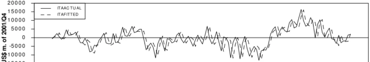
It is still possible to construct a fitted series for the current account, based on the fitted values obtained for the dependent variable in the OLS/IV estimations. However, since the term describing this dependent variable has a dynamic component, it is necessary to guess an initial value for the current account, and then iteract over the fitted values obtained initially. I arbitrarily choose the initial value of the fitted current account to be equal to the actual value in that period. The result of this procedure is presented in Figure B-2. The fitted series are reasonably close to the corresponding actual series in Italy and Turkey. However, in Australia, Spain and South Africa, the fitted series depart substantially from the actual series at some point.
5. CONCLUSION
The idea that some households simply spend whatever their current income is, came out in the literature as an attempt to explain the divergence between theoretical and empirical findings about consumption behavior. While Robert Hall’s random walk result suggested that only past consumption can help to predict future consumption, empirical studies consistently pointed to the current income as a good predictor. Since then, a great deal of effort has been paid to empirically assess the importance of the rule of thumb phenomenon in the economy, with mixed evidence. Surprisingly, none of these works investigated the issue on the basis of a current account theoretical model.
In this paper the concept of rule of thumb consumption is explored in the context of a small open economy. Two key assumptions are introduced in a standard intertemporal model of the current ac-count. The first one is the rule of thumb hypothesis, in which some individuals in the economy do not smooth consumption through their lifetime, in violation of the Permanent Income Hypothesis. The second one is that individuals form habits, in the sense that the past total average consumption in the economy affects the individual’s utility in the present. The paper estimates two parameters, namely, the share of domestic income that accrues to rule of thumb individuals and the coefficient of habit formation. We do so using current account data.
The model is estimated for five different developed and developing countries. The method
essen-tially relies on OLS and IV techniques. The estimates for the rule of thumb parameterλare surprisingly
high, varying roughly from 0.7 to 0.8, and are highly significant. The estimates for the habit formation
parameterθare quite small, sometimes negative, and in most of the cases non-significant. These
find-ings strongly support the view that rule of thumb consumption plays a key role in the determination of the aggregate consumption. Most importantly, they incorporate Weber’s (2002) criticism, which states that estimates of the rule of thumb parameter in models that do not account for habit formation are invariably upward biased.
Another important property of the model is the fact that it engenders a group of long-run
equilib-rium (or cointegration) relations between nonstationary variables that involve the parameterλ. The
existence of these cointegrating relations is tested empirically and the cointegrating vectors are
esti-mated, providing means to check the robustness of the OLS and IV estimates ofλ. The super consistent
estimates ofλfrom the long-run equilibrium relations are remarkably close to the OLS/IV estimates for
three countries, Australia, Turkey and Spain. For the two other countries, South Africa and Italy, the two econometric approaches yield results that are not highly similar. However, in all cases the estimates are very high, pointing out to the relevance of the rule of thumb behavior in the economy.
As a possible extension to this work, we suggest a departure from the idea thatλis a fixed co-efficient. It could vary through time and between countries. If Cushing (1992) argument that rule of thumb consumption proceeds from credit constraints suffered by the households is correct, then it is quite sensible to think that highly indebted individuals (or a highly indebted country) would have less
access to credit and would be more prone to be arule of thumber. An interesting idea would be to setλ
as a function of the country’s level of foreign indebtednessDt.
BIBLIOGRAPHY
Campbell, J. (1987). Does saving anticipate declining labor income? An alternative test of the permanent
income hypothesis. Econometrica, 55:1249–1273.
Campbell, J. & Mankiw, G. (1989). Consumption, income, and interest rates: Reinterpreting the time
series evidence. In Blanchard, O. & Fisher, S., editors,NBER Macroeconomics Annual, pages 185–214.
MIT Press, Cambridge, MA.
Campbell, J. & Mankiw, G. (1990). Permanent income, current income, and consumption. Journal of
Business and Economic Statistics, 8:265–280.
Constantinides, G. (1990). Habit formation: A resolution to the equity premium puzzle. Journal of
Political Economy, 98:519–543.
Cushing, M. (1992). Liquidity constraints and aggregate consumption behavior. Economic Inquiry,
30:134–153.
Frenkel, J. & Razin, A. (1996). Fiscal policies and growth in the world economy. Cambridge, third edition., MIT Press.
Ghosh, A. (1995). Capital mobility amongst the major industrialized countries: Too little or too much?
Economic Journal, 105:107–128.
Glick, R. & Rogoff, K. (1995). Global versus country-specific productivity shocks and the current account.
Journal of Monetary Economics, 35:159–192.
Gregory, A., Pagan, A., & Smith, G. (1990). Estimating linear quadratic models with integrated processes.
In Phillips, P., editor,Essays in honor of Rex Bergstrom. Blackwell Publishers, Cambridge.
Hall, R. (1978). Stochastic implications of the life-cycle permanent income hypothesis.Journal of Political
Economy, 86:971–988.
Ikeda, S. & Gombi, I. (1998). Habits, costly investment, and current account dynamics. Journal of
International Economics, 49:363–384.
Johansen, S. & Juselius, K. (1990). Maximum likelihood estimation and inference on cointegration with
application to the demand for money. Oxford Bulletin of Economics and Statistics, 52:169–209.
Nelson, C. & Plosser, C. (1982). Trends and random walks in macroeconomic time series: Some evidence
and implications. Journal of Monetary Economics, 10:130–162.
Obstfeld, M. (1992). International adjustment with habit-forming consumption: A diagrammatic
expo-sition. Review of International Economics, 1:32–48.
Sachs, J. (1981). The current account and macroeconomic adjustment in the 1970’s. Brooking Papers
Sheffrin, S. & Woo, W. (1990). Present value tests of an intertemporal model of the current account.
Journal of International Economics, 29:237–253.
Svenson, L. & Razin, A. (1983). The terms of trade and the current account: The
harberger-laursen-metzler effect. Journal of Political Economy, 91:97–125.
Weber, C. (2002). Intertemporal non-separability and “rule of thumb” consumption.Journal of Monetary
A. APPENDIX 1
Proof. of Proposition 1:
This is an extension for rule of thumb behavior of the main argument in Campbell (1987), Sheffrin and Woo (1990) and Ghosh (1995) papers.
Taking expression (9) in the text for the current account, we have
CAt=−Dt+1+Dt=Zt−Cpt−rDt (A-1)
whereZt= (1−λ)(Yt−Gt)−Itcan be defined as the net income of the permanent income
repre-sentative agent. Solving forDtin the backward direction
Dt=−
1 1 +r
∞ X
i=0
1
1 +r
i
[EtCpt+i−EtZt+i] (A-2)
Take expression (5) in the text using the definition of the forecast errorηt+1, and iterate it forwardly.
The result is
Cpt+i =Cpt+θ(Ct+i−1−Ct−1) +
i
X
j=1
ηt+j (A-3)
By taking expectations with the information set available at timet, the summation term in (15)
disappears and we have
EtCpt+i =Cpt−θCt−1+θEtCt+i−1 (A-4)
Substituting back into (14), we have
Dt=−
1
r(Cpt−θCt−1)−
1 1 +r
∞ X
i=0
1 1 +r
i
[θEtCt+i−1−EtZt+i] (A-5)
Solving forCptand substituting in the definition of the current account (13), we obtain
CAt=Zt−θCt−1−
r
1 +r
∞ X
i=0
1
1 +r
i
[EtZt+i−θEtCt+i−1] (A-6)
SubtractingP∞
i=0
1 1+r
i+1
[EtZt+i−θEtCt+i−1]in both sides of (18)
CAt=
∞ X
i=0
1
1 +r
i+1
[Et∆Zt+i+1−θEt∆Ct+i] (A-7)
Or, equivalently, substituting for the definition ofZt
CAt=
∞ X
i=0
1
1 +r
i+1
[(1−λ)(Et∆Yt+i+1−Et∆Gt+i+1)−Et∆It+i+1−θEt∆Ct+i] (A-8)
WithYt,Gt,It, andCtbeing I(1), their first-differences are I(0). Then, the equation above tells us
B. APPENDIX 2
The data used in the paper comes from the International Financial Statistic (IFS) data set, march/2003 version, published by IMF. The choice of countries for the analysis is based on the availability of data and on the fact that the theoretical model describes small and open economies. So big economies like the US or Japan were ruled out, in spite of the good quality of their data.
I took quarterly data, with the following time lengths: Australia, from 1959Q3 to 2002Q2; Italy, from 1970Q1 to 2001Q4; Spain, from 1975Q1 to 2002Q2; South Africa, from 1960Q1 to 2002Q3; and Turkey, from 1987Q1 to 2002Q1. The series of current account were obtained directly from the publication, in current US dollars, with no major modifications. The national account series, namely, GDP, aggre-gate consumption, aggreaggre-gate investment, and government expenditures, were collected in domestic currency, and then converted to US dollars using the end of period nominal exchange rate. These data follow the compilation of the System of National Accounts. So, aggregate consumption includes the Nonprofit Institutions Serving Households. Aggregate investment is the gross fixed capital formation (does not include the changes in inventories).
Ideally, the series for the debt in foreign currency should be described by a series of the international investment position of the country as a whole. IFS provides the series of assets and liabilities in US dollars, but typically for insufficient time lengths. So, I constructed the debt series by taking the last period of available data (subtracting the assets from the liabilities) and using the current account data
to iterate according to the formula Dt+1 = Dt −CAt. For the cases in which the international
investment position is available only with annual data, I did the iteraction considering that the last year available corresponds to the data of the fourth quarter of that year.
The final step was to use the US GDP deflator to express the series in constant prices referenced to the last period available for that particular country. So, all the series of Australia, for example, were expressed in US dollars of 2002Q2. Since the deflation was performed after the construction of the debt
series, the debt and current account series do not match exactly according toDt+1=Dt−CAt. That’s
Figure B-1: Actual and Fitted Dependent Variable
A u s tra lia
U S $ m. o f 2 0 0 2 /Q2
1 9 5 9 1 9 6 2 1 9 6 5 1 9 6 8 1 9 7 1 1 9 7 4 1 9 7 7 1 9 8 0 1 9 8 3 1 9 8 6 1 9 8 9 1 9 9 2 1 9 9 5 1 9 9 8 2 0 0 1 -1 5 0 0 0
-1 0 0 0 0 -5 0 0 0 0 5 0 0 0 1 0 0 0 0 1 5 0 0 0 2 0 0 0 0
AU SAC T U AL AU SF IT T ED
Ita ly U S $ m. o f 2 0 0 1 /Q4
1 9 7 0 1 9 7 2 1 9 7 4 1 9 7 6 1 9 7 8 1 9 8 0 1 9 8 2 1 9 8 4 1 9 8 6 1 9 8 8 1 9 9 0 1 9 9 2 1 9 9 4 1 9 9 6 1 9 9 8 2 0 0 0 -1 5 0 0 0
-1 0 0 0 0 -5 0 0 0 0 5 0 0 0 1 0 0 0 0 1 5 0 0 0
IT AAC T U AL
IT AF IT T ED
S p a in
U S $ m. o f 2 0 0 2 /Q2
1 9 7 5 1 9 7 7 1 9 7 9 1 9 8 1 1 9 8 3 1 9 8 5 1 9 8 7 1 9 8 9 1 9 9 1 1 9 9 3 1 9 9 5 1 9 9 7 1 9 9 9 2 0 0 1 -7 5 0 0
-5 0 0 0 -2 5 0 0 0 2 5 0 0 5 0 0 0 7 5 0 0 1 0 0 0 0
SPAAC T U AL
SPAF IT T ED
S o u th A fric a
U S $ m. o f 2 0 0 2 /Q3
1 9 6 0 1 9 6 3 1 9 6 6 1 9 6 9 1 9 7 2 1 9 7 5 1 9 7 8 1 9 8 1 1 9 8 4 1 9 8 7 1 9 9 0 1 9 9 3 1 9 9 6 1 9 9 9 2 0 0 2 -6 4 0 0
-4 8 0 0 -3 2 0 0 -1 6 0 0 0 1 6 0 0 3 2 0 0 4 8 0 0 6 4 0 0
SAF AC T U AL SAF F IT T ED
Tu rk e y
U S $ m. o f 2 0 0 2 /Q1
1 9 8 7 1 9 8 8 1 9 8 9 1 9 9 0 1 9 9 1 1 9 9 2 1 9 9 3 1 9 9 4 1 9 9 5 1 9 9 6 1 9 9 7 1 9 9 8 1 9 9 9 2 0 0 0 2 0 0 1 2 0 0 2 -6 0 0 0
-4 0 0 0 -2 0 0 0 0 2 0 0 0 4 0 0 0 6 0 0 0
T U R AC T U AL
Figure B-2: Current Account - Actual and Fitte d Values
C u rre n t A c c o u n t: A c tu a l a n d F itte d V a lu e s
A u s tra lia
U S $ m. o f 2 0 0 2 /Q2
1 9 5 9 1 9 6 2 1 9 6 5 1 9 6 8 1 9 7 1 1 9 7 4 1 9 7 7 1 9 8 0 1 9 8 3 1 9 8 6 1 9 8 9 1 9 9 2 1 9 9 5 1 9 9 8 2 0 0 1 -1 2 5 0 0
-1 0 0 0 0 -7 5 0 0 -5 0 0 0 -2 5 0 0 0 2 5 0 0 5 0 0 0
AU SAC T U AL AU SF IT T ED
Ita ly U S $ m. o f 2 0 0 1 /Q4
1 9 7 0 1 9 7 2 1 9 7 4 1 9 7 6 1 9 7 8 1 9 8 0 1 9 8 2 1 9 8 4 1 9 8 6 1 9 8 8 1 9 9 0 1 9 9 2 1 9 9 4 1 9 9 6 1 9 9 8 2 0 0 0 -1 5 0 0 0
-1 0 0 0 0 -5 0 0 0 0 5 0 0 0 1 0 0 0 0 1 5 0 0 0 2 0 0 0 0
IT AAC T U AL IT AF IT T ED
S p a in
U S $ m. o f 2 0 0 2 /Q2
1 9 7 5 1 9 7 7 1 9 7 9 1 9 8 1 1 9 8 3 1 9 8 5 1 9 8 7 1 9 8 9 1 9 9 1 1 9 9 3 1 9 9 5 1 9 9 7 1 9 9 9 2 0 0 1 -1 2 5 0 0
-1 0 0 0 0 -7 5 0 0 -5 0 0 0 -2 5 0 0 0 2 5 0 0 5 0 0 0
SPAAC T U AL SPAF IT T ED
S o u th A fric a
U S $ m. o f 2 0 0 2 /Q3
1 9 6 0 1 9 6 3 1 9 6 6 1 9 6 9 1 9 7 2 1 9 7 5 1 9 7 8 1 9 8 1 1 9 8 4 1 9 8 7 1 9 9 0 1 9 9 3 1 9 9 6 1 9 9 9 2 0 0 2 -6 0 0 0
-4 0 0 0 -2 0 0 0 0 2 0 0 0 4 0 0 0 6 0 0 0
SAF AC T U AL SAF F IT T ED
Tu rk e y
U S $ m. o f 2 0 0 2 /Q1
1 9 8 7 1 9 8 8 1 9 8 9 1 9 9 0 1 9 9 1 1 9 9 2 1 9 9 3 1 9 9 4 1 9 9 5 1 9 9 6 1 9 9 7 1 9 9 8 1 9 9 9 2 0 0 0 2 0 0 1 2 0 0 2 -5 0 0 0
-2 5 0 0 0 2 5 0 0 5 0 0 0
Table B-1: Augmented Dickey-Fuller Tests for the presence of Unit Roots in Current Account Data
Country ADFt-statistica,b Number of lags
Australia -6.20 *** 4
Canada 0.32 7
Denmark -2.02 3
Finland -1.77 5
Israel -1.94 4
Italy -3.11 4
Netherlands -1.18 3
Spain -2.93 4
South Africa -4.78 *** 4
Turkey -4.62 *** 2
R
odrigo
M.
Per
eira
Country CA Debt Cons Gov Inv GDP ∆CA ∆Debt ∆Cons ∆Gov ∆Inv ∆GDP Australia ADF t stat . -6.20*** -2.75 -2.75 -2.86 -2.71 -2.38 -6.93*** -4.68*** -14.61*** -7.12*** -11.72*** -12.61***
lags 4 5 0 2 1 0 5 4 0 1 0 0
Italy ADF t stat . -3.11 -1.84 -1.54 -0.99 -1.89 -1.87 -4.68*** -3.10 -8.78*** -9.04*** -7.99*** -8.83***
lags 4 5 2 2 2 1 3 4 1 1 1 1
Spain ADF t stat. -2.93 -3.08 -1.72 -1.80 -1.88 -1.83 -4.12*** -2.83 -8.88*** -8.81*** -8.41*** -8.71***
lags 4 5 0 0 0 0 3 4 0 0 0 0
South ADF t stat. -4.78*** -1.89 -2.28 -0.20 -1.05 -2.20 -6.05*** -4.83*** -6.24*** -11.13*** -12.15*** -6.13***
Africa lags 4 5 3 2 0 3 3 4 2 1 0 2
Turkey ADF t stat. -4.62*** -2.97 -3.51** -1.00 -2.82 -3.26* -6.06*** -4.26*** -5.49*** -10.48*** -5.56*** -4.70***
lags 2 2 4 3 4 4 2 2 4 -10.48*** 4 4
a: Significance at 1%, 5% and 10% are represented by ***, ** and *, respectively.
b: ADF tests are performed with a constant and a deterministic trend. The optimal number of lags is chosen using Ljung-Box tests.
RBE
Rio
de
Janeiro
v.
65
n.
2
/
p.
149–175
Abr
-Jun
Table B-3: Ordinary Least Squares Estimation of the Current Account Equation
Australia Italy Spain South Africa Turkey
r = 0.01 1 -λ 0.3061*** 0.2608*** 0.3077*** 0.2418*** 0.1885***
(21.416) (41.41) (8.1304) (14.052) (11.383)
-θ 0.0136 0.0087 0.0833* -0.0186 -0.0145
(0.7063) (1.0097) (1.6812) (-0.7560) (-0.3730)
centered R2
0,73 0,93 0,41 0,55 0,69
r = 0.02 1 -λ 0.3064*** 0.2600*** 0.3079*** 0.2414*** 0.1885***
(21.423) (41.0455) (8.0979) (13.987) (11.349)
-θ 0,0139 0.0080 0.0836* -0.0191 -0.0150
(0.7229) (0.9198) (1.6784) (-0.7751) (-0.3833)
centered R2
0,73 0,93 0.40 0,55 0,69
usable observations 170 126 108 169 59
Table B-4: Instrumental Variables Estimation of the Current Account Equation
Instruments Australia Italy Spain South Africa Turkey
1 to 3 1 -λ 0.3221*** 0.2615*** 0.2980*** 0.2339*** 0.1945***
(19.381) (39.484) (7.1202) (10.130) (11.355)
-θ 0.0834 0.0073 0.2498* 0.1558** -0.0258
(1.3616) (0.3852) (1.7930) (2.1599) (-0.5787)
r = 0.01 centered R2 0,71 0.93 0,35 0.41 0.70
Hansen’s J 19.68 20.07 24.58** 30.15*** 32.52***
(p-value) 0.1405 0.1278 0.0390 0.0073 32.52***
1 1 -λ 0.3116*** 0.2610*** 0.2409** 0.2525*** 0.1960***
(16.464) (36.991) (2.3560) (10.947) (11.260)
-θ ’-0.0726 0.0235 0.9289 0.0257 -0.0550
(-0.6048) (0.7876) (1.0428) (0.2736) (-1.1657)
centered R2 0,70 0.93 0.24 0.54 0,69
Hansen’s J 5.95 3.71 1.62 4.96 22.82***
(p-value) 0.2025 0.4468 0.8059 0.2915 0.0001
1 to 3 1 -λ 0.3225*** 0.2609*** 0.2983*** 0.2336*** 0.1945***
(19.354) (39.137) (7.1015) (10.110) (11.322)
-θ 0.0859 0.0037 0.2491* 0.1541** -0.0263
(1.3992) (0.1949) (1.7815) (2.1357) (-0.5886)
r = 0.02 centered R2 0.71 0.93 0.34 0,41 0.69
Hansen’s J 19.13 21.16* 24.15** 30.32*** 32.40***
(p-value) 0.1600 0.0976 0.0439 0.0069 0.0035
1 1 -λ 0.3127*** 0.2609*** 0.2434** 0.2526*** 0.1961***
(16.681) (37.117) (2.4357) (10.941) (11.227)
-θ -0.0634 0.0148 0.9013 0.0209 -0.0556
(-0.5336) (0.4966) (1.0356) (0.2223) (-1.1749)
centered R2 0.70 0.93 0.24 0,54 0,69
Hansen’s J 5.77 5.50 1.57 4.84 22.64***
(p-value) 0.2172 0.2397 0.8134 0.3042 0.0001
usable observations 167 123 105 166 56
Significance at 1%, 5% and 10% are represented by ***, ** and *, respectively. The numbers inside the brackets are the correspondingt-statistics. The set of instruments is based on lagged values of∆Yt−i,∆Gt−i,∆It−i,∆Ct−1−i, CAt−1−i. The tests are performed with lags from
Curr
ent
A
ccount
Dynamics
with
R
ule
of
Thumb
Consumers
1 lag
∆Yt−1 -0.174** (-2.396) 0.007 (0.093) -0.046 (0.828) -0.120** (-2.333) -0.346**** (-5.321) ∆Gt−1 0.553* (1.934) -0.217 (-0.911) -0.036 (-0.117) 0.200 (0.889) -2.230*** (-3.431)
∆It−1 0.525*** (2.836) 0.160 (0.673) 0.200 (1.256) 0.243 (1.482) 2385*** (4.783)
∆Yt−2 1.246*** (30.572) 1.340*** (58.198) 1.365*** (71.596) 1.263*** (28.710) 1886*** (16.642)
∆CAt−2 0.033 (0.295) 0.007 (0.180) 0.027 (71.596) 1.008*** (6.003) 0.543* (1.750)
R2 0.85 0.968 0.981 0.865 0.938
F statistic 187 732.05 1063.6 210.16 162.27
usable obs. 170 126 108 169 59
1 to 3 lags
∆Yt−1 -0.382*** (-4.120) -0.059 (-0.540) 0.039 (0.295) -0.021 (-0.233) -0.838*** (-6.120)
∆Yt−2 -0.142 (-1.476) -0.112 (-1.048) -0.251** (-1.993) -0.040 (-0.491) -0.573*** (-3.350)
∆Yt−3 0.046 (0.597) 0.044 (0.605) -0.012 (-0.211) -0.006 (-0.117) -0.196 (-1.613)
∆Gt−1 0.278 (0.877) -0.200 (-0.817) -0.202 (-0.587) 0.098 (0.370) 0.457 (0.653)
∆Gt−2 -0.020 (-0.064) 0.219 (0.889) 0.439 (1.325) 0.224 (0.800) 0.451 (0.534)
∆Gt−3 -0.155 (-0.519) 0.230 (0.907) -0.085 (-0.253) -0.260 (-1.066) 1.417** (1.906)
∆It−1 0.430** (2.243) 0.304 (1.202) 0.197 (1.002) 0.070 (0.398) 2.013*** (3.614)
∆It−2 0.165 (0.845) 0.010 (0.042) 0.084 (0.462) -0.068 (-0.402) 1.162** (1.960)
∆It−3 -0.097 (-0.490) -0.552** (-2.246) 0.052 (0.299) 0.287* (1.729) -0.430 (-0.709)
∆Ct−2 1.276*** (29.913) 1.355*** (54.731) 1.373*** (66.476) 1.272*** (28.878) 1.558*** (13.377)
∆Ct−3 0.484*** (3.614) 0.075 0.521 -0.085 (-0.543) -0.021 (-0.139) 0.539** (1.898)
∆Ct−4 0.233* (1.754) 0.072 0.505 0.241 (1.637) 0.050 (0.350) 0.250 (0.841)
∆CAt−2 -0.049 (-0.114) 0.054 0.975 0.101** (2.075) 1.626*** (7.207) 0.196 (0.592) ∆CAt−3 -0.438 (-0.868) -0.118* (-1.762) -0.058 (-1.171) -1.059*** (-4.008) 0.560 (1.348) ∆CAt−4 0.578 (1.356) 0.070 (1.241) -0.038 (-0.723) 0.058 (0.222) -0.893** (-2.580)
R2 0.867 0.973 0.983 0.885 0.978
F statistic 67.36 266.67 358.5 77.75 126.83
usable obs. 168 124 106 167 57
Significance at 1%, 5% and 10% are represented by ***, ** and *, respectively. The numbers inside the brackets are the correspondingt-statistics.
The set of instruments is based on lagged values of∆Yt−i,∆Gt−i,∆It−i,∆Ct−1−i, CAt−1−i. The tests are performed with lags from 1 to 3 (i = 1, i = 2,and i =3),
and with first lags(i= 1). The dependent variable is (∆Yt-∆Gt).
RBE
Rio
de
Janeiro
v.
65
n.
2
/
p.
149–175
Abr
-Jun
Table B-6: Ordinary Least Squares Estimation of the Tax Equation
Australia Italy Spain South Africa Turkey
τ 0.1596*** 0.1962*** 0.1615*** 0.1566*** 0.0529***
(23.341) (39.930) (40.861) (18.060) (4.5995)
centered R2
0,76 0,93 0,94 0,66 0,26
usable obs. 171 127 109 170 60
Significance at 1%, 5% and 10% are represented by ***, ** and *, respectively. The numbers inside the brackets are the correspondingt-statistics.
Table B-7: Augmented Dickey-Fuller test for the presence of unit roots in the estimated series of the
consumption of permanent income householdsb
Australia Italy Spain South Africa Turkey
ADF t stat.a -5.3693*** -2,1972 -1.9576 -2.1329 -2,6651
Critical Value (-3.4368) (-3.4455) (-3.4512) (-3.4370) (-3.4889)
(5% level)
lags 0 0 0 0 3
usable obs. 172 128 110 171 61
a: Significance at 1%, 5% and 10% are represented by ***, ** and *, respectively. The numbers inside the brackets are the correspondingt-statistics.
Curr
ent
A
ccount
Dynamics
with
R
ule
of
Thumb
Consumers
Country 4 lags 8 lags Null
Eigenvalue λ– max statisticb λ– trace statisticb Eigenvalue λ– max statisticb λ– trace statisticb Hypothesis (r)
Australia 0.0791 12.97* 13.82 0.0791 13.52* 14.54* 0
0.0062 0.085 0.085 0.0062 1.02 1.02 1
Italy 0.0273 3.10 3.13 0.0299 3.53 3.58 0
0.0002 0.02 0.02 0.0005 0.06 0.06 1
Spain 0.0268 2.88 2.90 0.0532 5.58 5.60 0
0.0002 0.02 0.02 0.0002 0.02 0.02 1
South Africa 0.0229 3.88 3.90 0.0271 4.48 4.49 0
0.0002 0.03 0.03 0.0001 0.01 0.01 1
Turkey 0.0885 5.28 5.31 0.1234 6.98 6.98 0
0.0005 0.03 0.03 0.0000 0.00 0.00 1
a: The test was performed without neither a drift vector nor an intercept in the cointegration vector. The critical values, as provided by Johansen and Juselius (1990) are 13.781 15.752 and 19.834 (null of r = 0), and 7.563 9.094
and 12.740 (null ofr= 1), for the levels of 90%, 95% and 99% of significance, respectively.
b: Theλ– max statistic tests the null hypothesis ofrand the alternative ofr+ 1cointegrating vectors. Theλ– trace statistic tests the null that there are no more thanrcointegrating vectors against the alternative of more thanr.
RBE
Rio
de
Janeiro
v.
65
n.
2
/
p.
149–175
Abr
-Jun
Table B-9: Johansen test for existence of cointegration between the debt, consumption of permanent
income households, investment, aggregate income and government expendituresa
Country Eigenvalue λ– max statisticb λ– trace statisticb Null Hyp.(r)
Italy 0.2590 36.88** 79.40** 0
(5 lags) 0.1612 21.63 42.53 1
0.1168 15.28 20.90 2
0,026 3.24 5.62 3
0,0192 2.38 2.38 4
Spain 0.3294 40.75** 103.76** 0
(8 lags) 0.2819 33.78** 63.01** 1
0.2124 24.36 29.23* 2
0.0450 4.70 4,87 3
0.0017 0.17 0.17 4
South Africa 0.2431 47.07** 92.03*** 0
(2 lags) 0.1554 28.54** 44,96 1
0.692 12.12 16,42 2
0.0242 4,14 4.31 3
0.0010 0.17 0.17 4
Turkey 0.8019 85.80** 128.37*** 0
(8 lags) 0.3466 22.55 42,57 1
0.2336 14.10 20.02 2
0.1043 5,84 5,92 3
0.0014 0.08 0.08 4
Critical Values (30.82 33.26 38.86) (65.96 69.98 77.91) 0
(10% 5% 1%) (24.92 27.34 32.62) (45.25 48.42 55.55) 1
(as provided by (18.96 21.28 26.15) (28.44 31.26 37.29) 2
Johansen & Juselius, (12.78 14.60 18.78) (15.58 17.84 21.96) 3
1990) (6.69 8.08 11.58) (6.69 8.08 11.58) 4
a: The test was performed without neither a drift vector nor an intercept in the cointegration vector. Significance at 1%, 5% and 10% are represented by ***, ** and *, respectively. The optimal number of lags was chosen trhough the multivariate generalization of the Schwartz Bayesian Criterion (SBC) applied over the VAR portion of the error correction model.