Universidade do Minho
Escola de Engenharia
Adrien Fernandes Machado
Finding new genes and pathways involved
in cancer development by analysing
insertional mutagenesis data
Universidade do Minho
Dissertação de Mestrado
Escola de Engenharia
Departamento de Informática
Adrien Fernandes Machado
Finding new genes and pathways involved
in cancer development by analysing
insertional mutagenesis data
Mestrado em Bioinformática
Trabalho realizado sob orientação de
Dr. Jeroen de Ridder
Dr. Isabel Rocha
Anexo 3
Declaração
Nome Adrien Fernandes Machado
Endereço Eletrónico [email protected] Número do Cartão de Cidadão 13909954
Título da Dissertação Finding new genes and pathways involved in cancer development by analysing insertional mutagenesis data
Orientador Professor Dr. Jeroen de Ridder Co-orientador Doutor Isabel Rocha Ano de Conclusão 2016
Designação do Mestrado Bioinformática
É AUTORIZADA A REPRODUÇÃO INTEGRAL DESTE TRABALHO APENAS PARA EFEITOS DE INVESTIGAÇÃO, MEDIANTE DECLARAÇÃO ESCRITA DO INTERESSADO, QUE A TAL SE COMPROMETE.
Universidade do Minho, 29 / 01 /2016 Assinatura:
"The purpose of life is to live it, to taste experience to the utmost, to reach out eagerly and without fear for newer and richer experience.".
Eleanor Roosevelt (1884 - 1962)
A
CKNOWLEDGEMENT
/ A
GRADECIMENTOS
First and foremost, I would like to thank my supervisor Dr. ir. Jeroen de Ridder for the opportunity to work this topic and for the continuous support, teaching and patience that he provided me during the this work.
A special thanks to the Delft Bioinformatics Lab, were all the work was done, for all the group meetings that enriched my knowledge about bioinformatics and great moments.
Gostaria de agradecer à Professora Isabel Rocha pelo apoio que me deu para a realiza-ção do Erasmus assim como a ajuda ao estabelecer esta nova parceria.
Toda esta jornada não seria possivel sem o apoio da minha família, dando a possibili-dade de realizar os meus objetivos e permitirem-me crescer profissionalmente. Um grande Obrigado aos meus pais e à minha irmã.
For the amazing housemates Cornel, Frank, Friso and Tom! Guys, you were incredible! Thank you for your fellowship along these months!
Aqueles que me acompanharam diariamente nesta aventura na Holanda - o gangtuga - um muito obrigado à Sara, Fred, João, Manel, Mariana, Marina, Sofia, Fitas.
Um agradecimento aos meus membros constituintes da equipa de camaradagem do Mestrado de Bioinformática 2013/14, em especial ao Daniel, Santa, Manel, Marisa, Lima, Tania e Vitor pelos conselhos e companheirismo destes últimos 2 anos.
À Joana e à Preta, um obrigado pela camaradagem e apoio ao longo destes últimos meses.
And, last but not least, thank you babe, for everything, all the support. You know.
A
BSTRACT
Cancer emerges from an uncontrollable division of the organism’s cells, creating a tumour. These tumours can emerge from any part of the human body. The increase of cellular divi-sion and growth can be created by mutations in the genome. Several methodologies are ap-proached, in the research, to finding new cancer genes. The insertional mutagenesis (IM) has been one of the most used, in which the mouse is infected by a retrovirus or a transpo-son, increasing the gene expression in the insertions’ vicinity.
The data used in work essay are a collection of independent studies of IM in mice. After its processing, the data has 3,414 samples, having information of 7,751 genes. Each sam-ple matches a type of cancer (colorectal, hematopoietic, hepatocellular carcinoma, lym-phoma, malignant peripheral nerve sheath, medulloblastoma and pancreatic).
The main goal of this project is to determine if there are specific genes for a particular type of cancer. And, if there are, which are the 15 most evolved genes for that type of cancer. Machine learning (ML) is a subject where its goal is to increase knowledge based on given experimental data, allowing it to execute predictions and accurate decisions. To an-swer our purpose, it is necessary the transform the data into a dissimilarity relation be-tween samples. Different approaches were used: two of them are known from the litera-ture (Hamming distance and Jaccard distance) and two new metrics were developed (Gene Dependent Method (GDM) and Gene Independent Method (GIM)). With these transforma-tions, unsupervised learning methods (such as Principal Component Analysis (PCA) and t-distributed stochastic neighbor embedding (t-SNE)) and supervised learning approach, testing different classifiers by crossed validation, were used.
The main results show that some genes may be specific to a particular type of cancer. Therefore, it is possible to create a ranking gene, according to its importance to a type of cancer. 105 genes are presented (15 genes of each type of cancer), of which 18 were not annotated yet and 19 have already been mentioned in the literature to be involved in the development of the selected cancer tissue. Afterwards it must be performed a proper in
vitro and in vivo validation.
Keywords: Cancer; cancer genes; insertional mutagenesis; machine learning.
R
ESUMO
O cancro surge da divisão incontrolável de células de um organismo, criando um tumor. Estes tumores podem surgir em qualquer parte do corpo do ser vivo. O aumento da divisão e crescimento celular pode dever-se a mutações no genoma. São várias as metodologias abordadas na investigação para a descoberta de novos genes de cancro. A mutação por inserção (IM) tem sido uma abordagem bastante utilizada, no qual o rato é infetado por um retrovírus ou um transposão, aumentando a expressão do gene que se encontra na vizinhança da inserção.
Os dados usados neste trabalho correspondem a uma coleção de estudos indepen-dentes de IM em ratos. Após o seu processamento, os dados contêm 3,414 amostras, tendo informação de 7,751 genes. Cada uma das amostras corresponde a um tipo de cancro (colo-rectal, tecido hematopoiético, carcinoma hepatocelular, linfoma, tumor maligno de bainha nervosa, meduloblastoma e pâncreas).
O objetivo principal deste projeto é determinar se existem genes específicos para um determinado tipo de cancro e, se sim, quais são os 15 genes mais envolvidos para o desen-volvimento do mesmo.
A aprendizagem de máquina (ML) tem como objetivo ganhar conhecimento com base em dados experimentais fornecidos, permitindo que este possa realizar previsões e de-cisões precisas. Para se responder ao objetivo, é necessária a transformação dos dados numa relação de dissimilaridade entre amostras. Foram usadas quatro abordagens: duas delas são descritas na literatura (a distância de Hamming e a distância de Jaccard) e duas novas métricas foram desenvolvidas (o método de gene dependente (GDM) e o método de gene independente (GIM)). A partir destas transformações foram usadas metodologias de aprendizagem não supervisionada (a Análise de Componentes Principais (PCA) e o
t-distributed stochastic neighbor embedding (t-SNE)), e a metodologia supervisionada,
tes-tando diferentes classificadores por validação cruzada.
Os resultados principais mostram que existem genes que poderão ser específicos para um dado tipo de cancro. Assim sendo, é possível criar uma ordenação dos genes de acordo com a sua importância face a um tipo de cancro. São apresentados 105 genes (15 genes para cada tipo de cancro), dos quais 18 ainda não foram anotados e 19 já foram mencionados na literatura por estarem envolvidos no desenvolvimento do cancro do tecido selecionado. Posteriormente deverá ser realizada a devida validação in vitro e in vivo.
Palavras-chave: Aprendizagem de máquina; cancro; genes de cancro; mutagénese por in-serção.
C
ONTENTS
Acknowledgement / Agradecimentos v
Abstract vii
Resumo ix
List of Figures xiii
List of Tables xv
Mathematical notations xix
1 Introduction 1
1.1 Motivation . . . 1
1.2 Objectives. . . 1
1.3 Structure of the dissertation . . . 2
2 Cancer research 5 2.1 Cancer . . . 5
2.1.1 The cancer cell evolution . . . 6
2.1.2 The cancer genes . . . 8
2.2 The research . . . 9
2.2.1 Discovering genes and pathways involved in cancer . . . 9
2.2.2 Insertional Mutagenesis . . . 10
3 Machine Learning 13 3.1 Learn from examples . . . 13
3.1.1 Classification . . . 14 3.1.2 Regression . . . 19 3.1.3 Clustering . . . 20 3.1.4 Dimensionality reduction . . . 21 3.2 Cross-validation . . . 23 3.3 Dissimilarity representation . . . 25 3.4 Feature ranking . . . 27 xi
xii CONTENTS 4 Data 29 4.1 Data generation . . . 29 4.2 Description . . . 29 4.3 Pre-processing . . . 32 5 Methodology 37 5.1 Data . . . 37 5.2 Data transformation . . . 37
5.2.1 Gene dependent method . . . 38
5.2.2 Gene independent method . . . 40
5.3 Unsupervised learning . . . 42
5.4 Supervised learning . . . 42
5.5 Gene Ranking . . . 43
6 Results and discussion 45 6.1 Unsupervised learning . . . 45 6.2 Supervised learning . . . 47 6.3 Ranking Genes . . . 49 7 Conclusion 53 7.1 Overview . . . 53 7.2 Limitations . . . 54 7.3 Recommendations . . . 54 Bibliography 55 A Appendix - Data transformation 71 A.1 Examples of distance metrics . . . 71
A.2 Entire data transformation . . . 72
B Appendix - Cross-validation values 73
L
IST OF
F
IGURES
2.1 Hallmarks of cancer. . . 8
2.2 Outline for cancer gene discovery using insertional mutagenesis. . . 11
3.1 Binary classification. . . 14
3.2 Example of Nearest Mean classification. . . 15
3.3 Example of k-Nearest Neighbour classification. . . 16
3.4 Example of Support Vector Machine classification in a linearly separable bi-nary dataset. . . 17
3.5 Example of a decision tree classification. . . 18
3.6 Example of a random forest classification. . . 19
3.7 Example of linear regression. . . 20
3.8 Cluster analysis . . . 21
3.9 Visualization of 2,000 samples of the MNIST dataset using PCA and tsne . . . 22
3.10 Representation of K -fold cross-validation. . . . 23
3.11 Representation of three ROC curves. . . 25
4.1 Organization of data generated. . . 30
4.2 Distribution of insertions represented in histogram and boxplot. . . 35
5.1 Example of a dataset and its respective distance matrix using GDM metric. . . 39
5.2 Example of a dataset and its the respective distance matrix using GIM metric. 41 5.3 Classifiers’ error rate. . . 43
5.4 Example of feature ranking using diff-criterion algorithm. . . 44
6.1 Result of PCA across the transformed data . . . 46
6.2 Result of t-SNE across the transformed data . . . 47
6.3 Results of CV across the transformated data . . . 48
A.1 Heat map of the distance matrices . . . 72
L
IST OF
T
ABLES
3.1 Confusion matrix used to tabulate the predictive capacity of
presence/ab-sence models. . . 25
3.2 Co-occurrence table for binary variables . . . 27
4.1 List of studies collected for this project regarding to insertional mutagenesis screens. . . 33
4.2 Samples’ size reduction of each tumour types . . . 34
5.1 Functions of PRTools used and their respective name. . . 42
6.1 List of the 15 genes more involved in a specific tumour type. . . 49
B.1 Cross-validation using the Hamming transformation . . . 74
B.2 Cross-validation using the Jaccard transformation . . . 75
B.3 Cross-validation using the GDM transformation . . . 76
B.4 Cross-validation using the GIM transformation . . . 77
L
IST OF
A
CRONYMS
2D two dimensions
3D three dimensions
AUC area under the curve
BCC Basal cell carcinoma
bp base pair
cDNA complementary DNA
CIS common insertion site
CV cross-validation
DNA deoxyribonucleic acid
FN False Negative
FP False Positive
GBM Glioblastoma multiforme
GDM gene dependent method
GIM gene independent method
HCC Hepatocellular carcinoma
HSC Hematopoietic stem cells ID3 Iterative Dichotomiser 3
IM insertional mutagenesis
kb kilobase
kNN k-Nearest Neighbour
MATLAB Matrix laboratory
ML Machine Learning
MuLV murine leukemia virus
MMTV mouse mammary tumour virus
MNIST Mixed National Institute of Standards and Technology MPNST Malignant peripheral nerve
sheath tumour
NMC Nearest Mean Classifier
PCA Principal Component Analysis
PCR polymerase chain reaction
RNA ribonucleic acid
ROC receiver operating characteristic
SCC Squamos cell carcinoma
SVM Support Vector Machine
T-ALL T-cell acute lymphoblastic leukaemia
TN True Negative
TP True Positive
t-SNE t-distributed stochastic neighbor embedding xvii
M
ATHEMATICAL NOTATIONS
Functions
acc Accuracy function
C A classifier function, where C (x) =b yb
d (a, b) Distance of a from b
dE Euclidian distance
dG I M Gene independent method distance
dGD M Gene dependent method distance
dH Hamming distance
dJ Jaccard distance
E RR Error function
F Example of a mapping function
H Entropy function
I (a, b) Indicator function where I (a, b) =
1 if a = b 0 if a 6= b
IG Information gain function
δ Indicator function whereδ(a,b) =
1 if a 6= b 0 if a = b
sg n(a) Signum function where sg n(a) = −1 if a < 0 0 if a = 0 1 if a > 0
SSE sum of squared errors function
Mathematical operations
a mean value of a
arg max
a
f (a)) the value of a that leads to the maximum of f (a)
arg min
a
( f (a)) the value of a that leads to the minimum of f (a) log2(a) logarithm with base 2 of a
n
P
i =1
ai The sum function from i = 1 to n : a1+ a2+ ... + an n
Q
i =1
ai The product function from i = 1 to n : a1× a2× ... × an
xx MATHEMATICAL NOTATIONS
Machine learning
D(X , Y ) Dataset D, with a set of vectors X and their respective label Y
Dt Training set X Set of vectors: X = {−→x1, −→x2, ..., −→xm} − →x i the it hvector, −→xi∈ X b
x new vector to be predicted
Y set of labels: Y = {y1, y2, ..., yz}
yi label of the it hvector, yi∈ Y
b
y the label predicted by a classifier C , C (x) =b yb
Xy1 Set of vectors belonging to the class y
1: Xy1= {−→x1y1, −→xy21, ..., −→xmy1}
− →xy1
i the i
t hvector of the class y1, −→xy1 i ∈ X
y1
A Set of attributes (or features), A = {a1, a2, ..., az}
ai the it hattribute, ai∈ A
A0 Set of mapped attributes, A0= {a01, a20, ..., anr0 }, nr < n
m number of vectors
my1 number of vectors belonging to class y
1
n number of attributes
nr number of attributes after mapping
z number of different labels
Probability
P (a) Probability of event a
P (a|b) Probability of event a given event b Sets
y ∈ Y y is an element of the set Y A ∩ B Intersection of the sets A and B
A ∪ B Union of the sets A and B
R Set of real numbers
Symbols
a ≡ b a is equivalent to b
1
I
NTRODUCTION
1.1.
M
OTIVATION
Cancer is the name given to an assembly of more than 100 diseases1. All these diseases can be very distinctive of each other. Nonetheless, they all have a similar starting point: an abnormal cell division, creating more cells than the body needs, producing a tumour.
Every year the number of new cases of cancer increases. In 2008, 12.7 million new reg-istrations and 7.6 million deaths as a possible result of this disease were estimated [1]. A recent study, analysing data from 2012, estimates a registration of 14.1 million new cases of cancer and 8.2 million deaths as a possible result of this disease [2]. This growth is caused essentially as a result of the populations’ rise, as well as to the exposition to risk factors.
Cancer is caused by changing the genetic information - the deoxyribonucleic acid (DNA)-of a cell. This alteration is called mutation and most (DNA)-of the time cells can repair it.
Cancer research is extremely important due the impact it can cause on our society. Analysing the changes of a gene or pathways, it is possible to predict which patients are likely to have a better or worse diagnosis.
1.2.
O
BJECTIVES
The key focus of this project is to improve understanding of biological processes that lead to cancer. The data collected contains information of exogenous DNA which integrates the mouse’s genome - insertional mutagenesis (IM). This integration will activate genes in its vicinity, in special, cancer genes.
1http://www.cancer.gov/about-cancer/what-is-cancer, accessed: July 2015
2 1.INTRODUCTION
The main biological question of the project is to determine which genes are likely to be a candidate as cancer genes to a specific type of cancer. To answer this question, the strategy is to use Machine Learning (ML).
Machine learning uses algorithms that can learn from data [3]. Classification methods allow to make predictions and decisions. For example, classification techniques have been used to extract cancer genes from large gene expression datasets [4–6]. IM screening data are represented by a very sparse Boolean matrix, and as such is very different from gene expression data. For this reason, the first problem is to know which classifier is suitable for application to sparse Boolean data. Several classifiers will be tested. To capture this in the classifier, the data will be transformed in a distance matrix. This evaluation will be performed using two classes, representing two distinct cancer types. To conclude, it will be evaluated feature selection methods to determine which genes interact in specific types of cancer.
1.3.
S
TRUCTURE OF THE DISSERTATION
This dissertation is divided into seven chapters. In this first chapter, a brief introduction of the motivation and the main aims of the work are provided.
Second chapter - Cancer research
Introduces several aspects related to cancer, as well as the research done to find new cancer genes.
Third chapter - Machine Learning
Presents an explanation of several important aspects of learning algorithms and their evaluation. To understand differences in the data it is explained some approaches to transform it. It is also discusses an approach to find important features from a dataset.
Fourth chapter - Data
Describes how the data was generated, how it was organized and explains the pre-processing performed, to have the final dataset.
Fifth chapter - Methodology
Explains the several steps of the work developed: the approaches used to transform the data; the unsupervised and supervised learning methods; as well as the ranking method.
1.3.STRUCTURE OF THE DISSERTATION 3
Sixth chapter - Results and discussion
Addresses the main results of this work: the visualization of the unsupervised learn-ing methods; the performances of selected classifiers used in supervised learnlearn-ing methods; and a list of potential genes that are involved in tumourigenesis.
Seventh chapter - Conclusion
Describes the main conclusions of the work, the limitations and recommendations for future work.
2
C
ANCER RESEARCH
2.1.
C
ANCER
Cancer is the name given to a group of diseases. All the different types of cancer arise with an unexpected aberrant cell division - neoplasia -, which disseminate to near tis-sues - metastesis. The Human body contains approximately 37 trillion and 200 million (3.72 × 10¹³) cells and all of them can originate a tumour [7]. Not all tumours lead to can-cer. In fact, tumours can be distinguished in two groups: benign and malignant. The first one does not have the ability to invade other tissues, which makes the removal a simple process. The second can spread to neighbour tissues. Even if the tumour is cut out, the organism still carries some cancer cells, which later can develop a new tumour.
Cancer is a genetic disorder. It is caused by changing gene expression, which controls the cell function. These changes can generate mutations. The probability of having a spo-radic mutation in each base pair (bp) is estimated to be 1 in 100 million (1.1×10⁻⁸)[8]. This value may seem low, but due the enormous quantity of bp that the Human genome con-tains, as well as, the massive number of cells each individual has in their lifetime and their risk behaviours, the probability increases largely. In addition, there are many agents which change DNA. They can be caused naturally by environmental factors due to physical (e.g. radiation), chemical (e.g. smoke) and biological (e.g. virus) causes, as well as, by genetic alterations (sporadic or hereditary) [9, 10].
Mutations happen all the time in our cells. In fact, during the cell cycle, cells have mech-anisms which can detect an error and repair them. If the cell cannot replace its damages, it will receive a signal to initiate the process to its death -apoptosis [11].
6 2.CANCER RESEARCH
Not all cancer cells are generated by mutations. Epigenetics is the study of cellular and physiological alteration caused by exogenous factors. In this situation, the alterations do not change the nucleotide sequence. Epigenetics alterations can change the expression of a gene, increasing or decreasing it.
2.1.1.
T
HE CANCER CELL EVOLUTIONThe cell - the basic structural, functional and biological unit of organisms – preserves, in-side it, one of the most important discovery in biological science, the DNA. This molecule contains the information that the cell needs. This information is stored in genes. One of the functions of the cell is to reproduce itself, dividing itself in two daughter cells and trans-mit its genetic information - cell cycle. It is estimated that this mechanism repeats between 50-70 billion cells per day in our organism to replace dead cells [12]. This process has two steps: interphase - the cell growth, accumulating compounds and duplicating its DNA; and
mitosis - the cell splits itself into two distinct cells. These two phases have checkpoints,
which ensures the appropriate replication of the DNA and division of the cell [13].
Before the transition from a normal to a cancer cell -tumourigenesis - can happen, the cell must overcome all its protections. It can be considered as an accelerated version of Darwin’s evolution theory: the individual receives an inherited genetic variation, it gets selective advantages and transmits it to its next generation [14–16]. In fact, if genes have different activities than usual, it will change, therefore, the cell’s activity and induce the ac-cumulation of several alterations in its DNA along its generations (during years or decades). They will overcome all checkpoints and gain some selective advantages compared to the normal cells [17]. With this accumulation, the cell will change its properties, and then, can evolve to a cancer phenotype [18].
To be considered as a cancer cell, the cell has to have several characteristics. Hanahan and Weinberg [19, 20] suggest that cancer cells can be summarised in 10 hallmarks (Fig-ure 2.1):
Six basic hallmarks, representing the fundamental basis of malignancy: Sustaining proliferative signalling
Normal cells regulate carefully the process of growth signals, insuring the cell home-ostasis. However, cancer cells can overcome this mechanism, for example, produc-ing more growth factor, increasproduc-ing the number of receptors on the cell surface and changing the signalling pathways.
Evading growth suppressors
pro-2.1.CANCER 7
cesses depend on the actions of tumour suppressor genes. Cancer cells become in-sensitive to mechanisms that regulate negatively the cell proliferation.
Resisting cell death
Due the DNA damage and other cellular stresses, normal cells may initiate apoptosis [11]. Most of cancer cells are less sensitive to similar stresses, avoiding apoptosis and contributing to the uncontrollable division.
Enabling replicative immortality
The number of division a cell can do is limited. These limits are usually established by telomeres (the ends of chromosomes). Along each cell division, in normal cells, telomeres get shorter until they are not able to divide. In contrast, in cancer cells, telomeres are preserved, allowing the cell to divide an unlimited number of times. Inducing angiogenesis
Angiogenesis is the process of creating new blood vessels, mediated mainly through vascular endothelial growth factor. It plays a critical role in tumour growth, supplying the cancer cells with oxygen and nutrients.
Activating invasion and metastasis
Metastasis is the cause of 90% of deaths from solid tumours [21]. Here, cancer cells may escape from the primary site and disseminate into distant organs. This process is not well understood, but it is known to involve a large number of secreted factors which breaks the tissue, allowing the invasion into blood vessels, and then, creating a new tumour in another place in the organism.
The acquisition of these hallmarks of cancer is made possible by two enabling charac-teristics:
Genome instability and mutation
Cancer cells achieve genome instability by increasing their mutation’s rate. They increase their sensitivity to mutagenic agents or breakdown of DNA repair macha-nisms.
Tumour promoting inflammation
Immune cells might infiltrate tumours and produce inflammatory responses. Inflam-mation can release chemicals into the tumour microenvironment, leading to genetic mutations and helping tumours acquire the hallmarks of cancer
8 2.CANCER RESEARCH
Figure 2.1: Hallmarks of cancer.
Characteristics the normal cell has to collect to achieve the cancerous phenotype. Figure adapted from Hanahan and Weinberg (2011) [20].
Deregulating cellular energetics
The uncontrolled growth and division of cancer cells may rely on the reprogramming of cellular metabolism, including increased aerobic glycolysis (known as the Warburg effect).
Avoiding immune destruction
The immune system is responsible for protecting the organism, including recogni-tion and eliminarecogni-tion of cancer cells. Evasion of this immune surveillance by weakly immunogenic cancer cells is an important emerging hallmark of cancer.
2.1.2.
T
HE CANCER GENESIt is widely accepted that tumourigenesis is a process which arises as a result of different activity of the genes present in the cell and they can differ between different types of can-cers. The main challenge that researchers face is understanding which genes must be active or inactive to stop the normal operation of the cell and arouses to cancer. Some of their names are known [22]. However, it is believed that most of them are still a mystery. The term "cancer gene" will be used throughout this dissertation to describe a gene for which mutations have been causally implicated in cancer. Cancer genes are commonly classified in two groups:
2.2.THE RESEARCH 9
Proto-oncogenes
Proto-oncogenes (e.g. myc and ras) are genes that incentives the cell growth. They turn to oncogene when they are mutated, being more active, allowing cells to grow more and surviving when they should not. Usually the overexpression of these genes is caused by gene amplification or chromosomal translocation [23].
Tumour suppressor genes
Tumour suppressor genes (e.g. p53) have as main purpose the reduction of cell pro-liferation. When these genes do not work correctly, the cell is able to grow out of control. This happens due to the mutation, causing loss of function of the gene.
It is important to understand that tumourigenesis develops as a result of activation of proto-oncogene, becoming an oncogene, and the inactivation of tumour suppressor genes. In general, to the tumour suppressor gene loss its function, it must be mutated in both alleles (recessive mutation)[24]. In contrast, since the mutation in oncogenes corresponds to the gain-of-function, most of its mutations involve only an individual allele (dominant mutations)[25].
2.2.
T
HE RESEARCH
Cancer formation results from gene mutations, which regulates the cell’s growth. Major tu-mours result either gain or loss-of-function of gene’s activity. Discovering which genes are involved in tumourigenesis allows, for example, the creation of drugs that can act against this abnormal gene or the protein encoded.
2.2.1.
D
ISCOVERING GENES AND PATHWAYS INVOLVED IN CANCERIn order to find new genes which leads to cancer’s hallmarks, several strategies are used. Most of them are tested in humans and in mouse [26]. Some techniques use tumour tissues from patients. On the other hand, a large part of the research uses animal models. The mouse is the biological model most used in research. It has a fast reproduction rate, a short life cycle and a small size, so it can be preserved in smaller spaces. In addition, the mouse is also physically and genetically similar to humans. Most genetics finding in mouse have a homology in human[27].
From all methods to discover new candidates to cancer genes, insertional mutagenesis (IM) has been a very efficient tool. The following work uses this approach in mouse and it is described below.
10 2.CANCER RESEARCH
2.2.2.
I
NSERTIONALM
UTAGENESISInsertional mutagenesis (IM) is a mechanism by which an exogenous DNA element inte-grates the genome of a host cell. It can be used in several fields of molecular biology, such as, gene therapy [28], gene regulation[29] and oncogene discovery [26]. As mentioned be-fore, the mouse is the most used model for cancer study, although IM has also been per-formed several different organisms, such as other vertebrates (e.g. chicken [30], zebrafish [31]), insects (e.g. Drosophila melanogaster [32]), plants (e.g. Arabidopsis thaliana [29] and rice [33]) and fungus [34].
HOW IT WORKS
In this technique, the mouse is infected by a retrovirus or a transposon. They will infect the healthy cells and integrates their genome in the host cells. By consequence, this inte-gration will deregulate genes in the vicinity, even in large distances [35], and can cause a perturbation of the phenotype. When the incorporation increases the expression of proto-oncogenes or decreases of tumour suppressor genes, it can result in an accelerated cell proliferation. The integration can alter the gene expression in different ways: either up-or downstream, changing its expression level and rarely the encoded protein; up-or within the gene, resulting in a different encoded protein or in its inactivation [36]. Regions in the genome that contain constantly insertions located in the same loci, in independent tu-mours, are referred as common insertion site (CIS). CIS show a significant overlap with human cancer genes (Figure 2.2)[37].
MECHANISM OF INSERTIONAL MUTAGENESIS
In order to find new cancer genes, two main mechanisms have been used : retrovirus and transposons. Retrovirus (e.g. murine leukemia virus (MuLV) and mouse mammary tumour virus (MMTV)) is a virus which its genome has a form of ribonucleic acid (RNA)and has the ability to convert its sequence into DNA by reverse transcription. Transposon (e.g. sleeping beauty and piggybac) is a DNA sequence that changes its position within the genome.
It is not known why this integration happens in the vicinity of a cancer gene. However, these mechanisms have integration biases [38].
2.2.THE RESEARCH 11
Figure 2.2: Outline for the cancer gene discovery using insertional mutagenesis (IM).
A- The mouse is infected with a retrovirus or transposon (1). After create a tumour (2), DNA is extracted (3),
amplified -by polymerase chain reaction (PCR)- (4), sequenced and mapped (5). In order to find clusters of insertions some statistical and bioinformatics analysis is performed, also knows as CIS(6). Genes in the vinicity of CIS are potential cancer genes (7). B- After find new candidates to be a cancer genes, they must be validated. This validation consists in verify if the gene transform normal cells in cancer cells. It can be tested in vitro (1) and/or in vivo(2). If the transformation happens, a cross-species to find the orthologues and homologs genes in human is performed (3). The final step is create a drug which can correct the abnormal gene expression (4).
3
M
ACHINE
L
EARNING
3.1.
L
EARN FROM EXAMPLES
Machine Learning (ML) is a branch of computer science emerged from the study of arti-ficial intelligence, pattern recognition and computational learning theory. This discipline is deployed in several fields, such as bioinformatics (e.g. evolution, systems biology, ge-nomics and others [39]), medical diagnosis [40], computer vision (e.g. image recognition [41]), speech recognition [42], document classification (e.g. spam [43]), music [44], games (e.g. checkers [45]) and others.
The main goal of ML is to extract knowledge from experimental data, allowing the com-puter to make accurate predictions and decisions.
All ML problems start with a dataset, a collection of information. This information, also called experiences or instances, are individual and independent examples given to the learner, representing observations. Each experience is characterized by its values, repre-senting a set of features. A feature (also known as attribute) is a measurement of something and can be nominal and numeric. Usually the dataset is defined as a matrix where the rows (m) are the instances collected, and the columns (n) are the features, representing the dimensionality of the data.
ML methods can be subdivided into two main groups based on the type of problem they can solve:
Supervised learning The learner gets a set of instances with their respective label, D(X , Y ), where D is the dataset, X is the set of vectors and Y the label. This method can be divided into two groups: classification and regression. The main difference between
14 3.MACHINELEARNING
these two analyses is the output type. In classification, the result is a discrete value, representing a class. In regression, the output is a continuous value and it depends on the independent variable given.
Unsupervised learning The learner gets a set of instances without labels, not being able to evaluate the method’s error. The approaches used are essentially clustering and
dimensionality reduction. The major difference between them is the way the
reduc-tion is done before their performance. In clustering, the number of experiences is reduced to generalize them. In dimensionality reduction, it is cutback the number of features, transforming them and reducing the dimensionality (preferably in two dimensions (2D) or three dimensions (3D)) to be easier to visualize.
However, there are more types of methods with more complex learning scenarios[3, 46].
3.1.1.
C
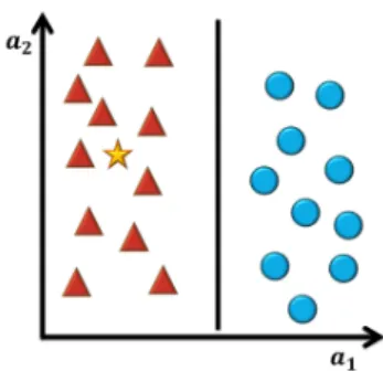
LASSIFICATIONClassification is used to identify in which set of categories a new experience can be labelled according to other experiences. The simplest classification problem is a binary classifi-cation. It creates a barrier (decision boundary) which separates the data in two different classes (Figure 3.1).
Figure 3.1: Binary classification.
Giving the data of two classes (triangles and circles)in two dimensions, where a1and a2
represent two features, it is possible to separate both classes with a straight line (linear classifier). According to this decision boundary created, it is possible to classify the new experience (star). The new experience belongs to the class of triangles.
The decision boundary is created by an algorithm, named classifier. This function takes the unlabelled examples and maps them into labelled, using internal data structures. The learning task in classification problems is to construct classifiers which are able to classify unseen examples (x) and give them a label (b y). A good classifier is the one who, given ab set of experiences - training set -, to create the knowledge, is able to predict/classify new examples correctly. There are a large number of classifiers and each one can have different performances depending on the dataset. Six learning classifiers are described bellow:
3.1.LEARN FROM EXAMPLES 15
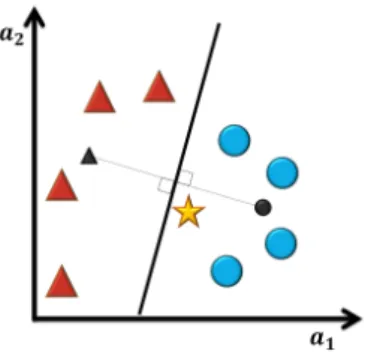
Nearest Mean Classifier
The Nearest Mean Classifier (NMC) [47], also known as Minimum Distance Classifier, is a linear classifier. This classifier calculates the centre of the class. A new experience is classified according to the closest distance of all class centre (Figure 3.2).
Figure 3.2: Example of Nearest Mean classification.
The centre of the classes are represented by the black triangle and circle. The classifier separates both classes creating a line equidistant to both centres. The test sample (star) should be classified as circle.
Giving a set of vectors representing the class y1(Xy1), containing m samples with size
n: Xy1= {−→xy1 1 , −→x y1 2 , ..., −→x y1 m} (3.1)
the centre of a class is determinated calculating the arithmetic mean ( ¯X ) of class’s
feature, ¯ Xy1= 1 my1 my1 X i =1 − →xy1 i (3.2)
To classify a new experiencex, it is calculated the minimum distance db E (Eucledian distance) betweenx and the centre of all classes ( ¯b XY).
b y = arg min { ¯Xy1, ¯Xy2,..., ¯Xyz}∈ ¯XY dE(x, ¯b XY) (3.3) dE(−→a ,−→b ) ≡ ||a − b|| ≡ s n X i =1 (ai− bi)2 (3.4)
k-Nearest Neighbour classifier
The k-Nearest Neighbour (kNN) classifier [48] classifies experiences based on closest training examples in the feature space. A new experience is classified by a majority
16 3.MACHINELEARNING
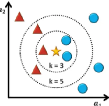
vote of the neighbourhood. The label more common of the k closest elements is the label of the new experience (Figure 3.3).
Figure 3.3: Example of k-Nearest Neighbour classification.
The test sample (star) should be classified either to the class of triangles or to the class of circles. If k = 3 (smaller dashed circle) it is assigned to the class of circles because there are 2 circles and only 1 triangle inside the inner circle. If k = 5 (bigger dashed circle) it is assigned to the class of triangles because there are 3 triangles and only 2 circles inside the inner circle.
Giving a training set Dt and a new experiencex, the method calculates the distanceb between the instancex and all training objects (X , Y ) ∈ Db t, where X represents the set of vectors and Y its labels. Once all experiences are sorted by the closest distance, the new experience is classified based on the majority class of its k nearest neighbours:
Majority voting:y = argmaxb
{y1,y2,...,yz}∈Y
k
X
i =1
I (yi, Y ), (3.5)
where yi are the labels of the nearest neighbours of classx, k is the number of theb neighbours, and I (yi, Y ) = 1 if yi= Y and I (yi, Y ) = 0 otherwise.
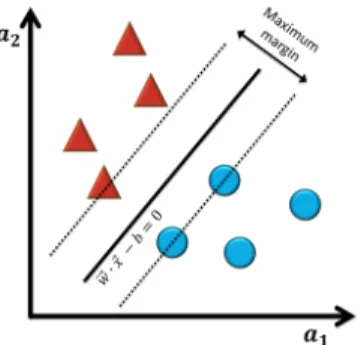
Support Vector Classifier
The Support Vector Machine (SVM) [49] is an algorithm which creates a hyperplane able to classify all training vectors in two classes. The best choice will be the hyper-plane that leaves the maximum margin from both classes (Figure 3.4).
The formula for the output of a linear SVM is
b
y = sg n(−→w · −→x + b) (3.6) where −→w is the normal vector to the hyperplane, −→x is the input value and b the
y-intercept. If sg n(−→w ·−→x +b) < 0, the new experience is classified by the class below the
3.1.LEARN FROM EXAMPLES 17
Figure 3.4: Example of Support Vector Machine classification in a linearly separable
bi-nary dataset.
The line is the hyperplan and the dashes lines are the margins. The main goal is to max-imize the distance between margins. Samples on the margin are called the support vec-tors.
Naïve Bayes Classifier
The Naïve Bayes classifier [50, 51] is based on Bayes’ theorem. This classifier assumes that the value of a feature is independent of the value of any other feature. This clas-sifier learns the conditional probability (Equation 3.7) of each class label yi given the
attribute ai:
P (yi|ai) =
P (ai|yi)P (yi)
P (ai)
(3.7) where P (yi|ai) is the posterior probability of class (target) given predictor (attribute);
P (yi) is the prior probability of class; P (ai|yi) is the likelihood which is the probability
of predictor given class; P (ai) is the evidence probability of predictor.
Classification is then done applying this probability of yi given the particular
in-stance of {a1, a2, ..., an} ∈ A. The predictable class is the one with the highest
prob-ability [52] b y = argmax yi∈{y1,y2,...,yz} P (yi) n Y j =1 P (aj|yi) (3.8)
Decision Tree Classifier
Decision tree [53] uses a tree structure. It breaks the dataset into smaller subsets until the result is a tree with a decision node or a leaf node. A decision node has two or more branches. A leaf node represents a classification. Decision tree requests several questions to attributes. Each answer will correspond to a branch. Once the decision tree is constructed, the classification is straightforward (Figure 3.5).
The simplest algorithm to construct decision trees is the Iterative Dichotomiser 3 (ID3) [53]. The major choice of ID3 algorithm is to find which attribute should be
18 3.MACHINELEARNING
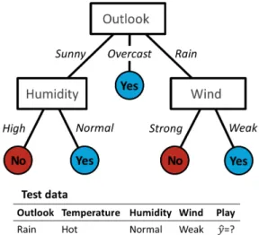
Figure 3.5: Example of a decision tree classification.
Nodes (rectangle) represent the features (outlook;humidity;wind), branches are the dif-ferent answers for a feature and leaves (circle) are the output (yes/no). The test sample would be sorted downs the rightmost branch of the decision tree and would be classified as a positive instance (it is possible to play).
the root, the most appropriate to classify examples. This algorithm uses a statistical test - Information Gain (IG) - that measures how well a given attribute classifies ex-periences. ID3 uses this measure to select among the different attributes at each step wile growing the tree.
Before calculating IG, the variable Entropy(H) hve to be determined:
H (Dt) = z
X
i =1
−P (yi) log2P (yi) , yi∈ Y (3.9)
where Dt is the training set for which entropy is being calculated, Y the set of classes
of Dt, z the number of different labels and P (yi) is the probability of yi in Y . If
H (Dt) = 0, the set Dt is perfectly classified.
IG is calculated according the following equation:
IG(Dt, A) = H(Dt) − X v∈V (A) #Dv #Dt H (Dv) (3.10)
where H (Dt) is the entropy of the training set Dt, V (A) is the set of possible values
for the attribute A, #Dv
#Dt is the proportion of a value v and the size of the training set Dt and H (Dv) is the entropy of the subset Dv.
Random Forest Classifier
3.1.LEARN FROM EXAMPLES 19
which creates additional data for training from the original dataset, creating several subsets, with random samples.
This classifier uses this approach to build a large collection of non-correlated trees. It selects a few combinations of samples with repetitions to create a decision tree. To predict a new element, all decision trees created are tested. Then, it counts how many time each class is predicted. The final result is the class with more votes.
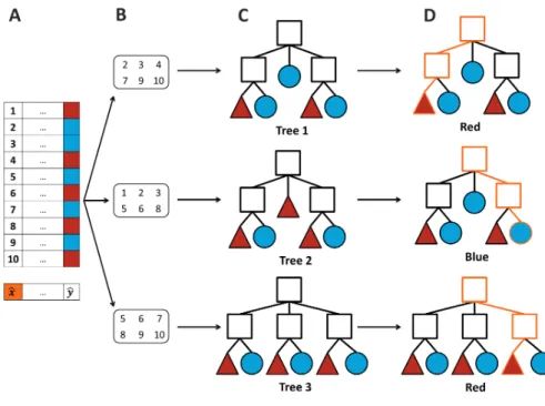
Figure 3.6: Example of a random forest classification.
A- The given dataset contains ten samples. Each sample has their respective label: blue or red. The main
goal is to predict which colour corresponds the new examplex, in orange. B- Three subsets containing sixb samples from the initial dataset is creted. C- For each subset, a decision tree is created. D- In each tree, the new examplebx is predicted. The output of tree 1, tree 2 and tree 3 is red, blue and red, respectively. Counting the number of votes of each label, the final result of this classification is red.
It is important to understand that no classifier is 100% precise to solve all ML problem. The dataset also affects the classifier’s performance. It also depends on the structure of the data (high/low bias and variances) and/or if a class has enough training experiences. A good way to find a classifier with a good performance is using cross-validation, testing their accuracy (see Section 3.2).
3.1.2.
R
EGRESSIONRegression is used to find a predictive modelling which tries to find a relation between a dependent (x) and independent variable (y). The model (function) created should fit in
20 3.MACHINELEARNING
real data points. In contrast with classification problems (see Section 3.1.1), the output value,y, is a continuous number.b
There are several kinds of regression methods, but the simplest one is the linear model, represented by a linear equation y = mx + b (Figure 3.7).
The model which has the best fit for a giving training data is calculated by minimizing the sum of the squares of the vertical distances from the data point to the line -
minimiza-tion of the sum of squared errors (SSE) [55]:
SSE =
m
X
i =1
(yi− ˆyi)2 (3.11)
where m is the number of experiences, yiis value of the dependent variable inxi and ˆyi
is the value of the dependent variable predicted by the model in xi.
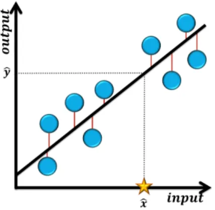
Figure 3.7: Example of linear regression.
The figure shows the linear regression line (black line), created from 9 training examples (circles). The connection between the data points and the point on the regression line (red lines) has the same xi value, denoting the distance used to calculate the sum of
squared errors.
The label of the new experience (star) isby,y ∈ R.b
3.1.3.
C
LUSTERINGClustering analysis is used to group a set of experiences into subsets, differentiating each group (cluster) according to a certain criterion. Examples in the same cluster are more similar to each other compared with objects in other clusters. There are several clustering algorithms and, for that reason, it is not easy to have an exact definition of cluster [56, 57]. However, it is typically mentioned as a method to “group unlabelled data objects”.
The main goal of this analysis is to understand how similar (or dissimilar) an individual experience is from other experiences. There are several different representations such as partitioned cluster and hierarchical cluster (Figure 3.8).
3.1.LEARN FROM EXAMPLES 21
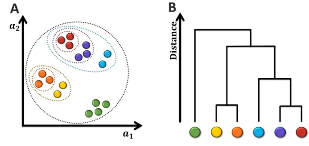
Figure 3.8: Cluster analysis.
A- Partitional clustering. The experiences are projected in a 2 dimensional plane. It is possible to group some
examples according to their similarity of the features a1and a2. B- Hierarchical clustering. Taking the clusters
of A, it is possible to calculate the distances between them and represent it in a diagram tree or dendogram. Each circle represents an experience and colours are used to distinguish clusters.
3.1.4.
D
IMENSIONALITY REDUCTIONIn Machine Learning problems, most of the data has a high dimension, in other words, a large number of features (n). In several domains it is important to visualize the data, but, with a high number of featuresm it can be difficult to extract information. For that reason, before analyse the data, a dimensionality reduction should be performed. This process takes the initial data and transforms into a lower-dimensional representation, preserving some properties of the initial form. The dimensionality reduction can be divided into fea-ture selection and feafea-ture extraction:
1. Feature selection
The feature space is reduced by selecting a subset of revelant features from the origi-nal data.
2. Feature extraction
The feature space from the original data is reduced through some functional map-ping. After feature extraction, the features are transformed and reduced. The new attributes are A0= {a10, a02, . . . , anr0 } , with (nr < n) and A0= F (A), where F is a map-ping function, which transforms the attribute A into A0, nr is the number of features after reduction. There are several feature extraction algorithms, but it will be present the Principal Component Analysis (PCA) and the t-distributed stochastic neighbor embedding (t-SNE):
Principal Component Analysis (PCA)
trans-22 3.MACHINELEARNING
formation. It will transform the data into a set of uncorrelated linear variables - principal components. The principal components are ordered according the degree’s variance. The first principal components contain most of the variation present in all of the original variables. The succeeding components have the highest variance compared to the preceding components (Figure 3.9 B)
t-distributed stochastic neighbor embedding (t-SNE)
t-SNE [61] is a nonlinear dimensionality reduction method. It is well suited to reduce high-dimensional data into the space of two or three dimensions. This analysis minimizes the divergence between two distributions: construct a dis-tribution that measures pairwise similarities, where similar samples have a high probability of being selected; and also construct a distribution that measures pairwise similarities of the corresponding low-dimensional maps (Figure 3.9 C). Given that PCA and t-SNE are unsupervised learning, the labels of the data are not used in the transformation. However, they are used to colour intermediate plots.
Figure 3.9: Visualization of 2,000 samples of the Mixed National Institute of Standards and Technology
(MNIST) dataset using PCA and t-SNE.
A- The MNIST dataset contains information of handwritten digits (from LeCun, Bottou, Bengio, and Haffner
(1998) [62]). PCA (B) and t-SNE (C) are dimensionality reduction algorithms, preserving the proprieties of the original dataset and allowing the visualization of the data. The figure shows that t-SNE has a better visualiza-tion compared to PCA.
3.2.CROSS-VALIDATION 23
3.2.
C
ROSS
-
VALIDATION
Cross-validation (CV) is a statistical method, used in preticting problems, to evaluate the accuracy (or error) of a model, being able to evaluate learning algorithms [63].
To perform this analysis, the data is splitted into two groups: the train set, used to learn a model; and the test set, used to validate the model.
There are a few different types of CV, but the most used is the K -fold cross-validation [64]. In K -fold cross-validation the data is subdivided into K identical sized folds. For each
K an iteration is performed: a different fold is used for a validation and the K − 1 folds to
learn. Each iteration has an error as an output. After all iterations, it is possible to calcu-late the average error rate of the model, giving an idea of how well the model generalizes (Figure 3.10).
Figure 3.10: Representation of K -fold cross-validation.
A- Dataset contains experiences of two classes. B- Data is reshuffled randomly to reduce the bias. C- Data is
subdivided into five identical sized subsets (K = 5). D- From the five folds created, four are used to train the model and the last fold for evaluation. E- The output is the average error rate of a classifier, giving an idea of how well is the classifier’s performance. In order to reduce the error rate, this process can be repeated, giving a more accurate average of each evaluation. In each repetition, the data is reorganized (B).
The number of folds (K ) to use is arbitrary, but there are some points to take into ac-count: if a large value is used, the bias of the true error rate estimator will be small, but the variance of the true error rate will be large and it will take too many time, due the low number of experiments in each fold; If a small number of folds is used, the computation
24 3.MACHINELEARNING
time is reduced, the variance of the estimator will be small, but the bias of the estimator will be large. A common choice for this method is use K = 10.
The output of each iteration is the estimated accuracy of the model. The accuracy of a classifier C is the probability of classifying correctly a random experience, i.e., acc =
P (C (x) =b y), whereb x is the experience andb y its class.b
In CV, the accuracy (acc) corresponds to the number of correct classifications, divided by the number of instances in the dataset [64]:
accCV = 1 m X (by,yi)∈Dt I (C (Dt,y), yb i) (3.12)
where m is the number of instances of the training set Dt, C (Dt, yu) is the mapping
function of the classifier C in the train set (Dt), havingy as a result, and I is an indicatorb function where I (a, b) = 1 if a = b and 0 otherwise.
The error (E RR) of a model can be calculated by:
E RR = 1 − acc (3.13) Another way to evaluate the viability of a model is using the area under the curve (AUC) of a receiver operating characteristic (ROC) curve [65]. Considering a two-class classifica-tion problem, in which the outcomes are pr esence or absences of a disease, it can have four possible solutions (Table 3.1): samples carrying the disease and the model can classify correctly its presence (True Positive (TP)), however, sometimes can happen to be classified as healthy (False Negative (FN)). On the other hand, some samples without the disease will be correctly classified as negative (True Negative (TN)), but some cases without the disease will be classified as positive (False Positive (FP)).
The ROC curve is created by plotting the False Positive Rate (or 1−Speci f i ci t y) against the True Positive Rate (or Sensi t i vi t y):
sensi t i vi t y = T P
T P + F N speci f i ci t y =
T N
T N + F P (3.14)
The curve always goes through two points: (0,0) and (1,1) (Figure 3.11). The model is considered better than other if the AUC is greater. If the AUC is equal to 1, it means that the test is 100% accurate because both specificity and sensitivity are 1, without false negative and false positive values. On the other hand, if a test cannot assess between correct and incorrect, the curve will correspond to a diagonal, where its AUC is equal to 0.5. The typical AUC of a ROC curve is between 0.5 and 1.
3.3.DISSIMILARITY REPRESENTATION 25 Table 3.1: Confusion matrix used to tabulate the predictive capacity of presence/absence models.
It can have four different outcomes: True Positive (TP) - presence observed and predicted by model; False Positive (FP) - absence observed but predicted as present; False Negative (FN) - presence ob-served but predicted as absent; True Negative (TN) - absence obob-served and predicted by model.
Predicted Presence Observed
Actual Presence TP FN
Absence FP TN
Figure 3.11: Representation of three ROC curves.
The green curve (AUC = 1) represents the best model, while the red curve (AUC = 0.5) represents the worst one. The blue curve is a positive predic-tive model.
The error (E RR) of a model can be calculated by:
E RR = 1 − AUC (3.15)
3.3.
D
ISSIMILARITY REPRESENTATION
In many cases it is not easy to evaluate a dataset and compare its samples. It can be con-venient to understand how different two samples are, that is, the distance (or dissimilarity) between them. Considering d (a, b) the dissimilarity of the sample a from b, then
d (a, b) > 0 if a 6= b
d (a, b) = 0 if a = b
d (a, b) = d(b, a)
d (a, b) ≤ d(a,c) + d(b,c)
(3.16)
If the dissimilarity measures satisfy the four conditions above, the dissimilarity measure is a metric and the term distance is usually used [66].
26 3.MACHINELEARNING
Compare all samples of a dataset will generate a distance matrix [67, 68]. Here, a dis-tance matrix is considered as a 2D array containing the disdis-tances, taken pairwise, between the samples of a dataset.
Matrix 3.17 represents an example of an array M(m×n), m rows and n columns, and it is filled with Boolean data, B = {0,1}. Each row is a vector (−→xi) and each column an attribute
(aj). M = a1 a2 a3 a4 a5 a6 ... an − →x1 B B B B B B . . . B − →x 2 B B B B B B . . . B − →x 3 B B B B B B . . . B − →x 4 B B B B B B . . . B .. . ... ... ... ... ... ... . .. ... − →x m B B B B B B . . . B (3.17)
Calculating the distance d through the matrix M, will map the distances between all samples of the dataset, creating a distance matrix (Matrix 3.18). The distance matrix is a square matrix with size m × m, symmetric, filled with non-negative elements and the diagonal elements are equal to zero. These proprieties are justified by the equations 3.16.
d (M) = 0 d (−→x1, −→x2) d (−→x1, −→x3) d (−→x1, −→x4) · · · d(−→x1, −→xm) d (−→x2, −→x1) 0 d (−→x2, −→x3) d (−→x2, −→x4) · · · d(−→x2, −→xm) d (−→x3, −→x1) d (−→x3, −→x2) 0 d (−→x3, −→x4) · · · d(−→x3, −→xm) d (−→x4, −→x1) d (−→x4, −→x2) d (−→x4, −→x3) 0 · · · d(−→x4, −→xm) .. . ... ... ... . .. ... d (−→xm, −→x1) d (−→xm, −→x2) d (−→xm, −→x3) d (−→xm, −→x4) ··· 0 (3.18)
There are many different ways to measure dissimilarity and, for that reason, there are many different dissimilarity transformations. It depends upon the application involved. For vectors of binary data, −→xi and −→xj, these may be expressed in terms of the number of
a, b, c and d where
a is equal to the number of occurrences of −→xi= 1 and −→xj= 1
b is equal to the number of occurrences of −→xi= 0 and −→xj= 1
c is equal to the number of occurrences of −→xi= 1 and −→xj= 0
3.4.FEATURE RANKING 27
This is summarised in Table 3.2.
Table 3.2: Co-occurrence table for binary variables
− →x i 1 0 − →x j 1 a b 0 c d
Two metrics often used are presented to map binary data into distances matrix: 1. Hamming distance
The Hamming dissimilarity [69] is defined by the ratio of mismatches among their pairs of variables: dH= #(−→xi6= −→xj) #[(−→xi 6= −→xj) ∪ (−→xi= −→xj)] ≡ b + c a + b + c + d (3.19) 2. Jaccard distance
The Jaccard dissimilarity[70] is defined by the ratio of mismatches among the non-zeros’s pairs: dJ= #[(−→xi 6= −→xj) #[(−→xi6= 0) ∪ (−→xj6= 0)] ≡ b + c a + b + c (3.20)
Equation A.1, in Appendix A.1, shows 9 examples to compare both metrics.
3.4.
F
EATURE RANKING
In Machine Learning, feature ranking is used to sort features, by relevance, for a certain class in a two class task. Different methods have been developed depending on the applica-tion [71]. However, this can bring some issues. Different methods will generate a different feature ranking of the same data.
A recent study [72] compares the three ranking algorithms for binary features to under-stand which one generates the most ’correct’ ranking. Using five artificial data and four real-life data they concluded that the diff-criterion algorithm got the most correct perfor-mance.
Diff-criterion [73] uses a distance between probability distributions of two classes. It estimates the importance of the it hfeature as:
− →
28 3.MACHINELEARNING
where p(ai= 1|y1) and p(ai= 1|y2) are the probability of a feature has a 1 in the classes
y1and y2.→−R is a vector containing the scores of a feature ai. Each score is a value between
-1 and -1. The higher the score, the greater importance. If a score is zero, it means the feature has the same probability of belonging in both classes. Sorting→−R , it is possible to have the
4
D
ATA
4.1.
D
ATA GENERATION
The following work was developed using an exclusive data collection, compiled from sev-eral studies (Table 4.1). They correspond to a compendium of IM screens in mice. The data from each study are available online and can be downloaded.
Each study uses several samples of tumour development. All of them were infected with an integration element (e.g. a retrovirus or a transposon). After that, insertions are identi-fied and mapped. For each gene, two windows with 10 kilobase (kb), up- and downstream of its location, were created. Window space is the name given to the distance between the first bp of a window upstream of the gene and the last bp of a window downstream of the gene (comprising the gene). It was verified, in all window spaces, whether it is carried an insertion or not. This results in a Boolean matrix: if an insertion is included in a window space, the gene will contain a 1, otherwise, the gene has a 0. All the information is stored in a .csv file (Figure 4.1).
4.2.
D
ESCRIPTION
This dataset contains information collected across 54 studies, obtained from 38 papers (Ta-ble 4.1). This compilation contains 7,037 samples of IM data organized in 14 types of can-cer. To the best of my knowledge, this is the first analysis, using DNA integration, to span an extensive number of independent tumours.
Each study contained between 17 and 3853 samples. They are related to one type of cancer, resulting in 13 specific ones and in one additional type labelled “Various”, which
30 4.DATA
Figure 4.1: Organization of data generated.
A- Each sample represents the genome of a cancer cell in the mouse. The mouse is infected by an integrating
element which inserts, randomly, pieces of DNA in the genome. After mapping the insertions, it is possible to identify their location. B- For each gene, two windows of 10 kb were created, located up- and downstream of the gene. In the area covered between windows - window space -, it was verified whether an insertion was integrated or not. C- The previous analysis was stored in a matrix, where for each sample it is identified which genes have an insertion in its vicinity. Insertion A is not covered by any windows. Insertion B (downstream of the gene), insertion C (within the gene) and insertion D (upstream of the gene) are captured by the window space of gene 3, gene 4 and gene 6, respectively. For this reason, entries for gene 1, gene 2 and gene 5 are 0, and gene 3, gene 4 and gene 6 are 1.
contain information of more than one cancer type. All types of cancer are described below:
Basal cell carcinoma
Basal cell carcinoma (BCC) it is the most common type of skin in cancer (80%)2and one of the most common type of cancer in humans. It is typically developed on ar-eas that have been exposed in the sun. It growths slowly and spreads to the nearest tissues, but it is rare to spread to other body parts.
Colorectal
Colorectal cancer starts in the colon or the rectum (part of the large intestine). It is the third most commonly diagnosed cancer in males and the second in females [2]. Glioblastoma
Glioblastoma multiforme (GBM) the most common type of cancer in the nervous system. It is formed from glial tissues of brain and spinal cord.
Hematopoietic
Hematopoietic stem cells (HSC) can develop all types of blood cells, producing an enormous number of blood cells every day.
2
4.2.DESCRIPTION 31
Hepatocellular carcinoma
Hepatocellular carcinoma (HCC) is the most common form of liver cancer. It is the second leading cause of cancer death in males [2].
Lymphoma
Lymphoma is a cancer which starts in the lymphoma system, a part of the immune system.
Malignant peripheral nerve sheath
Malignant peripheral nerve sheath tumour (MPNST) is a variety of soft tissue tu-mours. It is a rare tumour and appears in a neuron cell, the Schwann cells.
Mammary
Mammary cancer, also known as breast cancer in Human, is originated in the mam-mary gland. It is the most common cause of death in females.
Medulloblastoma
Medulloblastoma is the most common paediatric primary brain tumour. It can begin in the lower part of the brain and spread to the spine or other part of the body. Pancreatic
Pancreatic cancer starts in the pancreas. It is one of the most lethal type of cancer because usually is only diagnosed in advanced stages [74].
Sarcoma
Sarcoma is a type of cancer that begins in bone or in the soft tissues of the body (e.g. muscle, fibrous tissue, cartilage, etc).
Squamos cell carcinoma
Squamos cell carcinoma (SCC) is the second most common skin cancer, after BCC3. Like BCC it also develops on sun-exposed areas. It growth more likely into deeper layers of skin and are it is more frequent to spread to other body parts, comparing with BCC, but it is still uncommon.
T-cell acute lymphoblastic leukaemia
T-cell acute lymphoblastic leukaemia (T-ALL) starts in one of the lymphocytes’ cate-gory: T-cell. It is a type of white blood, present in the immune system.