Generalized entropy indices to measure
α
−
and
β
−
diversities of macrophytes
H. B. A. Evangelista∗, S. M. Thomaz∗, R. S. Mendes†, and L. R. Evangelista†
∗Departamento de Biologia (Nup´elia) and†Departamento de F´ısica and National Institute of Science and Technology for Complex Systems,
Universidade Estadual de Maring´a, Avenida Colombo, 5790 - 87020-900 Maring´a, Paran´a, Brazil
(Received on 17 February, 2009)
A family of entropy indices constructed in the framework of Tsallis entropy formalism is used to investigate ecological diversity. It represents a new perspective in ecology because a simple equation can incorporate all aspects ofα−diversity, from richness to dominance and can be also related to a measure of species rarity. In addition, a generalized Kullback-Leibler distance, constructed in the framework of a nonextensive formalism, is recalled and used as a measure ofβ−diversity between two systems. These tools are applied to data relative to the macrophytes collected from two not far apart arms of Itaipu Reservoir, in Paran´a River basin.
Keywords: Diversity indices, Ecology, Generalized entropy.
1. INTRODUCTION
Biodiversity is a central issue in ecology and biological conservation and has attracted the attention of ecologists and conservationists especially over the last two decades [1, 2]. The number (richness) of species has been largely used as a measure of biological diversity [3]. However, several in-dices were created to measure diversity, such as the Shannon-Wiener index (H) [4, 5], derived from information theory, and the Simpson index (D) [6], derived from probability theory. Both indices have been widely used since the 50’s and they are appealing because they summarize, in a single number, information on species richness (S) and species evenness (E). However, controversy on which index should be used exists in the literature, because diversity (and its broader meaning “biodiversity”) can not be fully captured in a single num-ber [7]. For these reasons, the introduction of a broader way to quantitatively measure diversity is tempting. In this di-rection, we agree with the idea that generalized diversity in-dices are superior to the traditional, one-dimensional ones, which are responsible for point descriptions of ecological as-semblages, as discussed in Refs. [8–10]. Consequently, it is necessary to explore the potentialities of generalized entropy indices within the ecological contexts in more details.
In this paper we first review the most common families of entropy indices that have been used in ecology in the last decades, with particular emphasis on the parametric Patil and Taillies indices (known in statistical physics as Tsallis en-tropy). This discussion puts in evidence how Tsallis entropy highly employed in physics and other areas of inquiry can be useful in ecology. Along with this family of indices, we will use a recently proposed index developed in the framework of this family, to explore its characteristics measures of di-versity in ecology with applications to aquatic macrophytes. The term “aquatic macrophytes” refers to a diverse group of aquatic photosynthetic organisms, all large enough to be seen with bare eyes [11]. Macrophytes are important in aquatic ecosystems, because they provide food and habitat for a va-riety of organisms, and interfere in the ecosystem function-ing [12–14]. Reservoirs are usually suitable for macrophytes development and they can deteriorate multiple uses of these artificial environments (navigation, water sports and losses in the generation of electricity). For this reason, in the Itaipu Reservoir as well as in other similar systems, investigation of the diversity of macrophytes has to be correctly addressed.
The data collected in two arms of the Itaipu Reservoir
are firstly analyzed to investigateα−diversity in the frame-work of Tsallis entropy indices, as extensively discussed in Ref. [15]. A further development of these ideas is the explo-ration of the concept ofβ−diversity. To accomplish this task, we use the generalized Kullback-Leibler distance, as given by Patil and Taillie [16] and Borland et al. [17]. In some sense, this follows the program started by Gorelick to extend Shan-non’s and Simpson’s indices to simultaneously account for species richness and relative abundance, but now we consider a continuous family ofqvalues [18].
This paper is organized as follows. In Sec. 2, we present in a summarized way the most common families of entropy indices that are also known in ecological applications, even if they have not been applied until now as intensively as they should be. The emphasis lies on the family constructed in the framework of Tsallis entropy formalism. In Sec. 3, we recall the definition of an alternative index, also based on Tsallis entropy, relevant to diversity and evenness. These indices are applied to a dataset (presented in Sec. 3.1) to quantitatively investigate theα−diversity of macrophytes. In Sec. 4, we review the derivation of the generalized Kullback-Leibler in-formation gain and discuss its relevance for the analysis of β−diversity. The mathematical tools built in this framework are applied to a dataset obtained not far apart in the Itaipu Reservoir as a measure of the dissimilarities among samples. Finally, some concluding remarks are drawn in Sec. 5.
2. GENERALIZED ENTROPY INDICES IN ECOLOGY
The use of families of indices have a long history in ecol-ogy [8, 19]. The first family was proposed by R´enyi (1961), who extended the concept of Shannon’s entropy by defining the entropy of orderα, originating a family ofα−diversity indices [19], in the form
R(α) = 1
1−αln
W
∑
i=1
pαi, for α≥0 and α6=1, (1)
wherepiis the probability of the stateiandW is the number
Brazilian Journal of Physics, vol. 39, no. 2A, August, 2009 397
Nα= W
∑
i=1 pαi
!1/(1−α)
, for α≥0 and α6=1. (2)
In the same direction, Dar´oczy (1970) and Acz´el and Dar´oczy (1975) also proposed an entropy family of typeαas [22, 23]:
Hα= 1
21−α−1 W
∑
i=1 pαi −1
!
, for α≥0 and α6=1.
(3) It is easy to show that the Shannon’s entropy is a limiting function ofHαwhenα→1. Patil and Taillie (1979) proposed a parametric diversity index familyβ, in the form [24]
∆β=
1
β 1−
W
∑
i=1 pβi+1
!
, for β6=0 and β≥ −1. (4)
The Patil and Taillie’s indices have been intensely studied re-cently in the context of statistical physics [25–27] and are usually written in the form:
Sq=
1−∑Wi=1p q i
q−1 , (5)
known as Tsallis entropy, whereq=β+1 is a real parameter which is considered non-negative to ensure thatSqis concave.
Motivated by these studies, Keylock (2005) explored these families of indices in an ecological context. A critical discus-sion of these indices was made by Jost (2006) [10]. Recently, a new index,Sq∗, was introduced as a unified way to measure ecological diversity and species rarity [15]. It is based on Patil and Tallies’s indices and the corresponding evenness. This family of indices (based on Tsallis entropy) captures multi-ple aspects of biodiversity and provides a better perspective that goes beyond the indices currently used in ecology. From this family, special diversity and evenness indices that bal-ance commonness and rareness, a practice still unemployed by ecologists, was proposed [15].
As a family of diversity indices, Eq. (5) interpolates the well known Simpson (q=2),
S2=1− W
∑
i=1
p2i, (6)
and Shannon- Wiener indices (q→1),
S1=− W
∑
i=1
pilnpi. (7)
In general, each specific application of the entropySqrequires
the determination of a particular value ofq. This is not an easy task, especially when dealing with statistical mechanical systems. On the other hand, a desirable measure of diver-sity has to take all the relevant aspects that characterize eco-logical systems into account, from richness to species domi-nance. Along these lines, when the possible values ofqare considered,Sqbecomes a family of diversity indices because
it embodies and accounts for the fundamental properties of the usual diversity indices in a simple and unified way. For instance, besides incorporating H and D, the Tsallis entropy can be used as a measure of richness because whenq=0, S1=S−1, withS=W andp0i =1, forpi6=0.
To end this section, it is necessary to emphasize, as we did before, that even if the idea of a family of indices and the indices themselves are known in ecology, they surely were scarcely applied in the last decades.
3. THE ALTERNATIVE INDEXSq∗
As underlined above,Sqrepresents a parametric family of
indices labeled byq, with some limiting values representing well-known indices that measure biological diversity. Simi-larly to what happened withSq, it is possible to introduce a
family of evenness indices also labeled byq[9]. This family is defined as
Eq=
Sq
Smax q
, (8)
where
Smaxq =1−W 1−q
q−1
represents the maximum value of Sq when the constraint
∑Wi=1pi =1 is imposed. As before, the limiting cases of
evenness can be obtained by considering particular values of q[15]. These indices will be used in this section to analyze part of the data described below.
3.1. The dataset
The Itaipu Reservoir, a major impoundment of the Upper Paran´a River located on the Brazil-Paraguai border, is colo-nized by a rich assemblage of aquatic plants. From January 2001 to July 2007, two arms located along the reservoir were studied (S˜ao Jo˜ao and S˜ao Vicente). Sixty stands (30 per arm) were surveyed from a boat, at constant and low velocity. In each stand, two independent samplers spent 10 min observing or collecting aquatic macrophytes for identification. To repre-sent the time employed in the analysis prerepre-sented in this paper, we fixed the time for the first sample (made in both arms in January 2001) ast1=0 month. After that, 13 other samplings
were made (described in Table I), just to give an idea of the oscillation between summer and winter in the collects. The relative abundance (pi) of each species was measured as:
pi=
ni
∑Si=1ni
,
whereniis the number of stands in which the speciesiwas
recorded.
398
TABLE I: Periods in which the samples were collected in two arms of the Itaipu Reservoir: S˜ao Vicente River and S˜ao Jo˜ao River. The time for the first sample was fixed, for reference, ast1=0 and the
others are given in months on the right column.
Sampling Time (months)
January, 2001 t1=0
June, 2001 t2=5
January, 2002 t3=11
August, 2001 t4=18
February, 2003 t5=24
July, 2003 t6=29
January, 2004 t7=35
July, 2004 t8=41
January, 2005 t9=47
July, 2005 t10=53
February, 2006 t11=60
July, 2006 t12=65
January, 2007 t13=71
July, 2007 t14=77
(see Sec. 3.1). The trend of the curve is the expected one, showing the existence of a minimum that definesq∗. Each sample, corresponding to a given arm, is associated to a mini-mum. The temporal variation ofq∗is depicted in Fig. 2 for all
0.0 0.5 1.0 1.5 2.0 2.5 3.0 0.94 0.96 0.98 1.00 E v e n n e s s ( E q ) q
0 12 24 36 48 60 72
0.2 0.3 0.4 0.5 0.6 q * t n (months)
0 12 24 36 48 60 72
0.90 0.93 0.96 0.99 E v e n n e s s e s t n (months)
FIG. 1: Evenness indices Eq versus q for the data described in
Sec. 3.1: January, 2001 (dotted line), January, 2002 (solid line), and February, 2003 (dashed line). The minima in these curves corre-spond toq=q∗.
samples shown in Table I. It is remarkable thatq∗remained below the valueq=1 in every month, exhibiting oscillations (minima in summer and maxima in winter). Notice that this pointq=q∗ defines the maximum deviation of the perfect equitability (Eq=1.0) of a given sample. For this reason
and because the negative relationship betweenq∗andSwas demonstrated, the indexEq∗, defined forq=q∗, was inter-preted as a parameter associated with species rarity[15].
For comparative purposes, in Fig. 3Eq∗and the usual even-nessE(i.e., the evenness related to the Shannon’s index) are shown for S˜ao Vicente River along time.
The absolute values of these indices are clearly different, as expected, because they correspond to different values ofq, but their values were significantly correlated (Pearson = 0.66). However, the new indexEq∗enhanced the temporal variations characterizing the sample. This behavior reinforces the
con-0.0 0.5 1.0 1.5 2.0 2.5 3.0 0.94 0.96 0.98 1.00 E v e n n e s s ( E q ) q
0 12 24 36 48 60 72
0.2 0.3 0.4 0.5 0.6 0.7 q * t n (months)
0 12 24 36 48 60 72
0.90 0.93 0.96 0.99 E v e n n e s s e s t n (months)
FIG. 2:q∗versus thetn(in months) corresponding to the samples
de-scribed in Sec. 3.1. A continuous line in this and subsequent graphs was drawn to visualize trends.
0.0 0.5 1.0 1.5 2.0 2.5 3.0 0.94 0.96 0.98 1.00 E v e n n e s s ( E q ) q
0 12 24 36 48 60 72
0.2 0.3 0.4 0.5 0.6 q * t n (months)
0 12 24 36 48 60 72
0.90 0.93 0.96 0.99 E v e n n e s s e s t n (months)
FIG. 3: Evennesses indicesEq∗ (dotted line ) andE1 (solid line)
versustnfor the dataset described in Table I.
clusion thatEq∗can be helpful as a new index, to be added to the classical ones, in order to form a family of indices and to achieve a better description of the diversity.
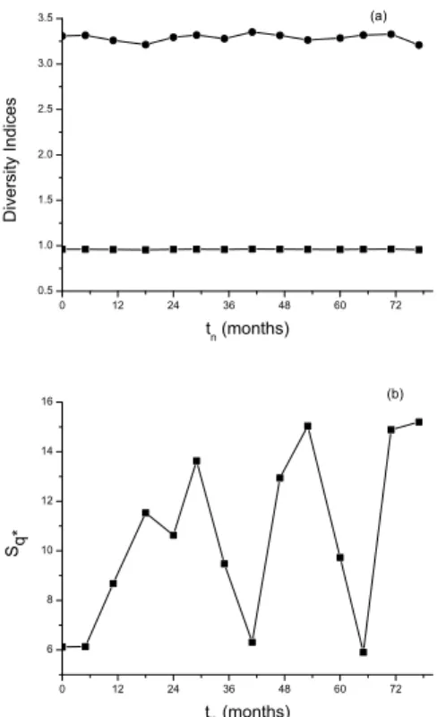
In Fig. 4, the diversity indices corresponding to the data of Table I are shown. The new index, Sq∗ (Fig. 4b) is shown along with the classical ones of Shannon and Simp-son (Fig. 4a). Again, it is remarkable that Sq∗ is the one that best evidences the oscillations and the marked variations along time. In fact, the Simpson index (S2) seems to remain
essentially constant (CV=0.064) whereas the Shannon index (S1) oscillates with low amplitude (CV=0.339) as compared
withSq∗(CV=8.99).
4. THE GENERALIZED KULLBACK INFORMATION GAIN
As stated before, the Shannon’s entropy can be obtained as a particular case of Eq. (5) whenq→1, thus yielding Eq. (7), which can be rewritten as
S= W
∑
i=1
Brazilian Journal of Physics, vol. 39, no. 2A, August, 2009 399
0 12 24 36 48 60 72 0.5
1.0 1.5 2.0 2.5 3.0 3.5
D
iv
e
r
s
ity
In
d
ic
e
s
t n
(months)
(a)
0 12 24 36 48 60 72 6
8 10 12 14 16
S
q
*
t n
(months)
(b)
FIG. 4: Diversity indices versustnfor the data of Table I: (a) the
classical indicesS1=H(Shannon, circles) andS2=D(Simpson,
squares) and (b) the new index,Sq∗.
whereIi=−lnpi, which is the information content of
out-comei. The change of information,∆Ii, between two sets of
measurements can be defined as
∆Ii=− lnp′i−lnpi, (10)
wherep′idenote the first set of measurements andpithe new
set of measurements. The so-called Kullback-Leibler infor-mation gain orrelative entropyis defined as [17]:
K(p,p′) = W
∑
i=1 pi∆Ii=
W
∑
i=1 piln
pi
p′i. (11) Similarly, it is possible to show that a generalized Kullback-Leibler measure follows naturally from the standard deviation of the Kullback entropy by employing the nonextensive for-malism. One obtains [17]:
Kq(p,p′) = W
∑
i=1 pqi 1−q
p1i−q−p′1i−q
= W
∑
i=1 pi
1−q "
1−
p
i
p′
i
q−1#
. (12)
Whenq→1, we get Eq. (11); forq=0,Kq(p) =0. It is
pos-sible also to introduce a distance connected with Simpson’s measure (q=2):
K2(p,p′) =1−
W
∑
i=1 p2i p′
i
. (13)
In ecology, α−diversity has been defined as the species diversity within community plots [28]. Thus, the analy-sis presented in previous section concerns specifically with α−diversity. The β−diversity is, however, defined as the amount of turnover in species composition from one loca-tion to another [29]. To investigateβ−diversity some indices have been proposed. Among them, we mention the qualitative Sorensen’s index, defined as
Cs=
2N SA+SB
, (14) whereNis the number of species found in both sites andSA
andSBare the number of species found in sitesAandB,
re-spectively. The other index is the quantitative Morita-Horn index:
CmH=
2∑iNiANiB
(∑iNiA2/NA2+∑iNiB2/NB2)NANB
, (15)
whereNAandNBare the total number of individuals andNiA,
NiBare the number of individuals of theith species in sites
AandB, respectively. These are similarity indices, i.e., they can be used to quantify community changes due to natural succession or environmental perturbations [30].
In another direction, dissimilarity measures between com-munities have been proposed [29]. In particular, T´othm´er´esz suggested summarizingβ−diversity using the distribution of plot-to-plot dissimilarities within a vegetation sample instead of scalars [31]. Some years before, Wilson and Mohler [32] proposed to measure compositional change along gradients with data on species relative abundance, by means of the “gradient rescaling method”. By expanding on an idea of T´othm´er´esz [31], Ricotta and Avena [29] proposed to characterize β−diversity for data on species relative abun-dances based on the distribution of Kullback’s information-theoretical distance of single plots from the pooled sample.
0.0 0.5 1.0 1.5 2.0 2.5 3.0 -5
0 5 10 15 20 25 30 35
l
n
K
q
(
p
,p
'
)
q
0 12 24 36 48 60 72
0 8 16
l
n
K
q
(
p
,p
'
)
t n
(months)
400 H. B. A. Evangelista et al.
As a natural extension of this idea, in this paper we propose to quantitatively investigate some aspects of theβ−diversity by using the generalized Kullback-Leibler distance, Eq. (12), introduced above. To illustrate the usefulness of this ap-proach, we applied this measure to the dataset presented in Sec. 3.1. We used two close arms of the Itaipu Reservoir just to emphasize the power ofKqto enhance the
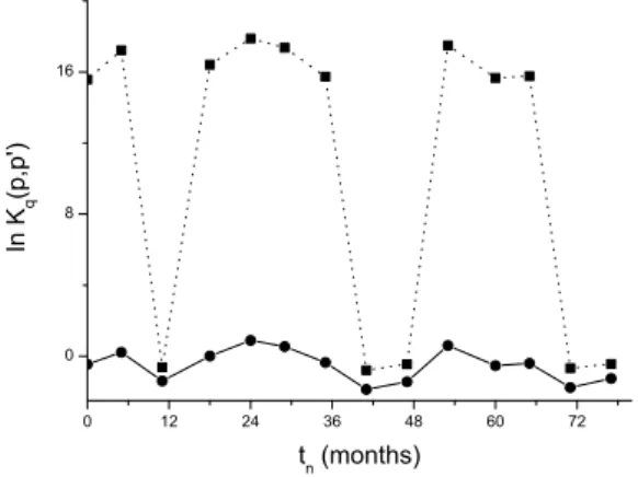
dissimilar-ities among these two (in principle) similar commundissimilar-ities (as shown in Fig. 5). In Fig. 6, the logarithm of the Kullback-Leibler distance correspondent to the Shannon and Simpson indices is shown.
0.0 0.5 1.0 1.5 2.0 2.5 3.0 -5
0 5 10 15 20 25
l
n
K
q
(
p
,p
'
)
q
0 12 24 36 48 60 72
0 8 16
l
n
K
q
(
p
,p
'
)
t n
(months)
FIG. 6: Logarithm of the Kullback-Leibler distance vs. time for Shannonq→1 (circles) and Simpsonq=2 (squares) limits.
Both indices have the same overall trend. However, the distance connected withq=2 (Simpson) enhanced the dif-ferences between the two systems. On the other hand, it is clear that the similarity between the two sites is low for Jan-uary 2002, JanJan-uary 2005, and JanJan-uary 2007. This is the sum-mer period, in which the two systems present similar diver-sity. However, in the winter, represented by the months June 2001, July 2003, and July 2005, the values ofK2(p,p′)are high, indicating that the species found in these arms are dif-ferent. These preliminary results confirm the potentiality of a generalized distance to be associated with theβ−diversity
investigations in ecology.
5. CONCLUDING REMARKS
As we have emphasized above, the idea of a family of di-versity indices is not novice in ecology, but it has not been explored in all its potentialities. After reviewing the main families proposed in this endeavor, we used a family of in-dices constructed in the framework of the Tsallis’s entropy formalism to investigate diversity of aquatic macrophytes in two arms of the Itaipu Reservoir. To accomplish this task, we used the new indices linked with this formalism. In particular, we used an index connected with the special value ofq=q∗, the parameter characterizing this family of entropy indices, whose meaning still deserves investigation. We found that the indices associated toq∗, i.e., the value for which the evenness presented its maximum deviation from the perfect equitabil-ity, can be particularly useful as an additional information to exploreα−diversity in ecological samples. In addition, we also discussed the possible role of a Kullback-Leibler dis-tance in investigations ofβ−diversity. In this sense, this paper represents a step further to carry on a detailed investigation of a broad aspect of diversity, at least for two fundamental rea-sons: i) it demonstrates the applicability of an unified tool to describeα−diversity by means of a set of unified parameters, embodying diversity from richness to dominance and species rarity; ii) it permits us to face aspects ofβ−diversity in the same framework and with the same mathematical tools used for α−diversity. We are then convinced that this approach, based on a nonextensive formalism, can be relevant not only in the framework of statistical physics but will also find broad applications in ecological systems.
Acknowledgments
Many thanks are due to the Brazilian agencies, CNPq and Capes, for partial financial help. H. B. A. Evangelista thanks PDTA/PTI Parque Tecnol´ogico de Itaipu for a fellowship.
[1] E. O. Wilson and F. M. Peter (eds),Biodiversity(National Aca-demic Press, Washington DC, 1988).
[2] G. Moorel and E. O. Wilson, Nature405, 254-256 (2000). [3] A. E. Magurran, Ecological diversity and its measurement
(Princeton University Press, Princeton, 1988). [4] C. E. Shannon, Bell Syst. Technol. J.27, 379 (1948).
[5] C. E. Shannon and E. W. Weaver,The mathematical theory of communication(University of Illinois, 1949).
[6] E. H. Simpson, Nature163, 688 (1949).
[7] A. Purvis and A. Hector, Nature405, 212-219 (2000). [8] G. L¨ovei, Community Ecology6, 245, 2005. [9] C. J. Keylock, Oikos109, 203 (2005). [10] L. Jost, Oikos 113, 363 (2006).
[11] P. A. Chambers, P. Lacoul, K. J. Murphy, and S. M. Thomaz,
Hydrobiologia595, 9 (2008).
[12] R. G. Wetzel,Limnology(Saunders College Publishing House, Philadelphia, 1983).
[13] C. M. Duarte, D. Planas, and J. Pa˜nuelas,Macrophytes: taking control of an ancestral home, in R. Margalef, (ed). Limnol-ogy now: a paradigm of planetary problems(Elsevier Science, Amsterdam, 1994).
[14] F. Esteves,Fundamentos de Limnologia(Interciˆencia, FINEP, Rio de Janeiro, Brasil, 1998).
[15] R. S. Mendes, L. R. Evangelista, A. A. Agostinho, S. M. Thomaz, and L. C. Gomes, Ecography31, 450 (2008). [16] G. P. Patil and C. Taillie, J. Am. Stat. Soc.77, 548 (1982). [17] L. Borland, A. R. Plastino, and C. Tsallis, J. Math. Phys.39,
6490 (1998).
[18] R. Gorelick, Ecography29, 525 (2006). [19] B. T´othm´er´esz, J. Veg. Sci.6, 283 (1995).
[20] A. R´enyi, On measures of entropy and information. In: 4th Berkeley Symposium on Mathematical Statistics and Probabil-ity(Berkeley, USA, 1961) edited by J. Neyman.
Brazilian Journal of Physics, vol. 39, no. 2A, August, 2009 401
[22] Z. Dar´oczy, Inform. Control.16, 36 (1970).
[23] J. Acz´el and Z. Dar´oczy,On Measures of Information and their Characterizations(Academic Press, New York, 1975). [24] G. P. Patil and C. Taillie,An overview of diversity. In:
Ecologi-cal Diversity in Theory and Practice(International Cooperative Publishing House, Fairland, MD, 1979), edited by J. F. Grassle, G. P. Patil, W. Smith, and C. Taillie.
[25] C. Tsallis, J. Stat. Phys.52, 479 (1988).
[26] C. Tsallis, R. S. Mendes, and A. R. Plastino, Physica A261,
534 (1998).
[27] C. Tsallis, Braz. J. Phys.39, 337 (2009).
[28] R. H. Whittaker, Ecological Monographs30, 279 (1960). [29] C. Ricotta and G. Avena, Plant Biosystems137, 57 (2003). [30] A. Ludovisi and M. I. Taticchi, Ecological Modelling192, 299
(2006).