Modeling of Low-altitude Quasi-trapped Proton Fluxes
at the Equatorial Inner Magnetosphere
A.A. Gusev,
1,3G.I. Pugacheva,
2U.B. Jayanthi
1, and N. Schuch
2 1Instituto Nacional de Pesquisas Espaciais/INPE, 122-970, S ˜ao Jos´e dos Campus, SP, Brazil
2
Southern Regional Space Research Center; INPE, Santa Maria, Brazil
3
Space Research Institute/IKI, Russian Academy of Sciences, Moscow, Russia
Received on 15 January, 2003.
A secondary proton radiation belt can be observed in the equatorial region between the upper atmosphere and the interior edge of the main radiation belt. It is thought that the protons appear there in a result of ionization of energetic neutral hydrogen atoms coming from the internal area of the traditional radiation belt where they were born in charge exchange collisions of the trapped protons with the cold hydrogen of the gecorona. The process of formation of this secondary belt is numerically simulated in this paper assuming this charge exchange−
re-ionization mechanism. Standard models of the trapped radiation, of the atmosphere and geocorona were used to simulate the source and the exospheric media. Experimental data were used for charge transfer cross sections. Result of simulation agrees very good with the experimental observation.
1
Introduction
An experiment APEX - Monitoring of Alpha, Proton and Electron fluxes in the inner magnetosphere is being devel-oped for the French-Brazilian Microsatellite (FBM) to be deployed in 2003. The satellite orbit with an inclination of 6-10◦and a height of≈700kmwill permit continuous mon-itoring of ion and electron fluxes essentially in the equatorial region of the innermost magnetosphere. The studies will be focused on the dynamical phenomena like fast radial diffu-sion and precipitation of the fluxes and their dependence on solar, magnetospheric and atmospheric conditions.
In the present work we consider the nature and character-istic of energetic proton environment in the equatorial region under the main radiation belt where the orbit of the FBM will pass. These protons are considered now also as a useful tool for observation of global magnetospheric dynamics.
The presence of a secondary radiation belt consisting of energetic protons and located in the interface region be-neath the classic radiation belt and above the terrestrial at-mosphere was established by Moritz [1] and Hovestadt [2]. They observed protons in the energy range of 0.25-1.65 M eV between the altitudes from 400 to 1000 km. Miz-era and Blake [3] extended observation to lower energies measuring a spectrum of 12.5-500keV protons in the 400-470kmaltitude range. Low-altitude rocket [4] and satellite measurements [1] indicate that the protons are concentrated at 90◦pitch angle with a magnitude independent of altitudes
above ∼300 km. More recently, Guzik et al. [5] discov-ered a strong altitude dependence in the flux of equatorial protons with energies from 0.6 to 9M eV at lower altitudes between 170 and 290 km. We [6] examined the integral proton fluxes in the energy range 0.64-35M eV atLvalues from 1.05 to 1.15 over a 3-year period and observed abrupt
flux enhancements of up to three orders of magnitude lasting for 1-3 days, and flux decreases of two orders of magnitude lasting a few monthes.
The observations reported were performed at low alti-tudes where geomagnetic drift shells are unclosed. Due to that we can formally regard the protons as quasi-trapped. In reality their lifetime is determined by charge exchange losses that is much shorter than the drift period. Due to that the fact that the drift shells are unclosed does not affect the flux magnitude of the protons, which is determined essen-tially by the same factors as inside the traditional radiation belt at closed drift lines.
Simple solid state detectors used mainly for detection of the protons inkeV −M eV range in those experiments can only measure a sum of neutral and re-ionized fluxes. The neutral/re-ionized flux ratio strongly depends on the ion en-ergy decreasing from∼10 at 10keV to∼0.1 at 100keV. To select exactly neutrals one needs to eliminate proton back-ground. It is usually done with constant magnets (see for ex-ample [4] ), that permits latitude-longitude mapping of the proton source. Contrary to that the simple telescopes mea-sure a quasi-trapped flux that reflects the neutral flux aver-aged over a trajectory of Larmour rotation of the protons in the geomagnetic field.
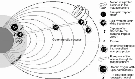
A permanent, intense source needed to reproduce this population is identified as a charge exchange process of pro-tons captured in the radiation belt and ring current region [1] as is illustrated in Fig. 1: Source trapped protonsH+
con-fined in the magnetosphere undergoes a charge exchange in-teraction with relatively cold (∼ 1000◦K) ambient neutral
atom A0
e.g.H+
+ A0→H0 + A+
(reaction1in Fig. ). Af-ter neutralization these protons appear as a fast non-thermal hydrogen neutral atomsH0
neutral they are not affected or confined by the geomagnetic field and can travel in any direction. If they head earthward, there is a chance that they will collide with atmospheric neu-tral atoms and lose the electron in reaction of re-ionization H0+ A0 →
H++ A0
+ e−. (reaction2in Fig. 1)
appear-ing now as positive ion ofH+
i.e. proton. If the angle
be-tween velocity of the proton and geomagnetic line direction is sufficiently close to 90◦the proton can be trapped i.e. can perform geomagnetic drift along a line of the geomagnetic equator belonging to a definiteL-shell. (Geomagnetic equa-tor is defined as a plane crossing geomagnetic field lines in the point of minimum strength of the geomagnetic field.)
Motion of a proton confined in the magnetosphere
Energetic trapped proton
Cold hydrogrn atom of the geocorona
Capture of an electron by the energrtic trapped proton
Electron
An energetic neutral i.e. neutralized energetic proton
Free pass of the neutral through the magnetosphere
Atomic oxygen of the upper atmosphere
Re-ionization of the energetic neutral
Figure 1. A scheme of formation of quasi-trapped proton population beneath the radiation belt. The geomagnetic field is approximated with field of a tilt shifted dipole. Geomagnetic equator is defined as a plane crossing geomagnetic field lines in the point of minimum strength of the geomagnetic field.
The mechanism described above provides a direct link between the radiation belt and the upper atmosphere at mid-latitudes and low-mid-latitudes. Because of their origin the char-acteristics of the neutral and quasi-trapped proton fluxes are closely related with those of the radiation belt proton popu-lation. It permits permanent monitoring the general dynam-ics of the ring current region and traditional proton radiation belt [6,7] where direct measurements are still fragmental and rather complicated due to presence of intensive destructive radiation.
A noticeable variations of neutral and/or quasi-trapped fluxes correlated with geomagnetic storms were reported by Moritz [1], Mizera and Blake [3], Voss et al.[4], and Greenspan et al. [7]. Orsini et al. [8] simulated hy-drogen and oxygen neutral fluxes basing on the data of AMPTEE/CCE measurements [9] and found that the neutral flux magnitude depends on the level of geomagnetic activity. The transport of the neutral particles between the inner radiation belt and the upper atmosphere through the charge exchange and the following free flight across geomagnetic field lines was used for explanation of the observation of mid and low latitude precipitations [10-13]. Some estima-tions result to a flux of precipitating neutral hydrogen of 10 keV energy up to2·1051/cm2s sr keV
during magnetic storm [14]. The penetrating neutral particles deposit consid-erable energy to the thermosphere heating the atmosphere. Intensive precipitation of H ions ofM eV energy range were observed by Gusev et al. [6] when magnitude of
precipitat-ing fluxes exceeded1041/cm2s sr
in energy range 0.64-35 M eV.
The goal of the present work is simulation of quasi-trapped proton fluxes in the assumption that they are pro-duced in charge exchange−re-ionization process using the standard model of radiation belt. It will permit both to check the hypothesis of their origin and the radiation belt model it-self. Until now no comparison of the physical model and experimental results has been done. This work is a part of the project of experimental study of energetic proton popu-lation in the innermost region of the magnetosphere (APEX) which will be performed on board a French-Brazilian satel-lite.
2
Parameters of the model
In the present work we only consider neutrals born with ve-locity vectors placed in the plane of the geomagnetic equator and directed to the center of the Earth. It means that we con-sider only the neutrals born by the trapped protons at the top of a geomagnetic field line with velocity vector placed in the meridian plane perpendicular to field line i.e. possessing a pitch angle of 90◦.
dFN(E, x)
dx =jT P(E, x)P(E, x)−FN(E, x)D(E, x) (1) The first term in the right part of the equation describes production of the neutrals in the charge exchange reaction of trapped protons with exospheric cold atoms:
• jT P(E, x)is a directed flux of the trapped protons in 1/cm2
s sr M eV, • P(E, x) =X
i
σi10(E)n
i(x) 1/cm ,
• σi
10(E) cm 2
is a cross section of electron capture from a cold neutral specie iof the exosphere or at-mosphere by energetic proton of energyE,
• ni(x) 1/cm3
is a density of neutral atoms of speciei. The second term describes the losses of the energetic neutrals:
• D(E, x) =X i
σi01(E)n i(x)
1/cm,
• σi
01(E)nicm 2
is a cross section of loss of electron by energetic neutral in collision with a neutral atom of specieiof the exosphere or the upper atmosphere.
We take into account atomic and molecular hydrogen, helium, nitrogen and oxygen as main species constituting the atmosphere and exosphere.
To calculate a flux of energetic neutrals in a point of ob-servation one needs to integrate the equation 1 along a path of view from the outer magnetospheric boundary to the point of observation.
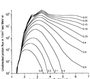
Figure 2 presents the intensity of the source proton fluxes trapped in the plane of the geomagnetic equator. The unidirected flux magnitudes were derived from the standard model of the trapped radiation AP8 (see Acknowledgement) describing distribution of global (i.e. coming from all the direction of the 4π solid angle) energetic proton fluxes in the magnetosphere of the Earth. The model contents a 3-dimensional table of magnitudes of the integral global fluxes J(> E, L, BP/B0)in1/cm2sec
in points characterized by proton energyE,L-shell number (i.e. distance from the ge-omagnetic dipole center of the top of the gege-omagnetic field line passing through the point ) and a ratioBP/B0of mag-netic field strengthBP in the given point to magnetic field strengthB0at the top of the same field line. One more part of the model is a FORTRAN code for access and interpo-lation of the data of the table. To convert global fluxes to unidirected onesj⊥((> E, L, BP/B0)perpendicular to the
magnetic field line in the point with magnetic strengthBPa following expression from Roederer [15] was used
⌋
j⊥(> E, L, Bp/B0) =
Bp3/2 2π2
B0
Z
Bp d dB
·
J(> E, L, Bp/B0) Bp
¸
dB (B−Bp)1/2
⌈
Figure 2. Intensity of the unidirected differential proton fluxes
jT P(E, L)trapped in the equatorial plane. The numbers next to
the curves mark proton energy inM eV.
Integration is performed along the magnetic field line from the pointBp to the point B0. A problem of a sin-gularity in the pointB = Bp was resolved by decreasing the integration step in the singularity vicinity until reaching a desirable convergence.
The procedure was performed for the each point of the AP8 table and a global flux value in the point was substi-tuted with a value of the related unidirected flux. It permits to implement the same FORTRAN code of access and inter-polation both for extracting and interinter-polation the global and the unidirected fluxes. Thus this new table can be considered as a model of the unidirected trapped proton fluxes.
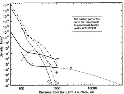
Figure 3. Atmospheric and exospheric densities according MSISE-90 model and Chamberlen geocoronal model.
Figure 4. Charge transfer cross section for hydrogen ions according to Allison, [1958]. σ10- charge exchange cross section i.e. that of
electron capture by energetic proton;σ01- ionization cross section i.e. that of loss of electron by an energetic neutral.
Rairden et al. [17] according a spherically symmetric geo-coronal model of Chamberlen [18]. (Geocorona is a tenuous cloud of exospheric neutral hydrogen enveloping the Earth. It can be observed as a faint glow around our planet, pro-duced in resonant scattering of solar Lyman alpha radiation.) Figure 4 shows energy dependences of charge transfer cross section for the most important atomic atmospheric constituents measured by Allison [19]. To obtain the molec-ular cross sections for the energies>1keV the atomic ones must be multiplied by the factor of 2 [20].
The only neutral specie present in significant numbers in the Earth’s magnetosphere at the altitudes of the confine-ment region is atomic hydrogen. Due to that the reactionH+ + H0 →H0
+ H+
is considered as a main source of ener-geticH0. On the other hand, the same mechanism of charge exchange is an important mechanism of losses of ions con-stituting the classical radiation belt (see for example [21] ).
One can see that charge exchange cross section σ10
rapidly decreases with the energy for proton energy exceed-ing 10keV. Due to that the resulting spectrum of the neu-trals is significantly steeper than the parent trapped proton spectrum.
neutraliza-tion. No new protons are produced there because the parent neutral flux is exhausted after passage through the above at-mospheric matter. The other part of the re-ionized protons trapped at higherL-shell can perform noticeable number of turns around the Earth until loss their energy in Coulomb scattering or suffer neutralization collisions in the residual atmosphere. But there they can not be distinguished from the parent protons of the radiation belt.
The magnitude of the re-ionized proton flux during the geomagnetic capture is determined by the balance between the source (i.e. ionization of the neutral flux) and losses due to neutralization and Coulomb scattering. Fig. 5 demon-strate mean characteristic times of the processes involved.
Figure 5. Character times of the processes involved in formation of the neutral and quasi-trapped proton fluxes: re-ionization (ion-ization), neutralization (charge exchange), Coulomb scattering (en-ergy losses). Lifetime until Coulomb scattering is defined as time until losses of 30% of the initial energy of the proton.
One can see that lifetime until Coulomb scattering ex-ceeds that until neutralization by about one order of mag-nitude at practically all the altitudes. However a real life-time can be different because the altitude of the geomag-netic equator along which the proton drifts also varies. If the proton drifts sufficiently rapid its lifetime will be deter-mined by the losses at the smallest altitude of the geomag-netic equator, where the atmospheric density is higher. On the unclosed drift trajectories i.e. on those with the mini-mal altitude< 100 km, the proton lifetime is determined by the time which the proton spends at higher altitudes. It is approximately equal to the proton drift period around the Earth shown also in Fig. 5. It is also one order of magnitude higher compared to the neutralization lifetime for the alti-tudes<1000km. At higher altitudes the drift motion does not result to particle losses because of small exospheric den-sity. Due to that the corresponding lifetime is also incom-paratively higher than those of the other processes. It means that a quasi-trapped proton dies close to the point where it was produced in re-ionization collision.
In reality the drift period is determined not by a local altitude as the Fig. 5 shows, but by anL-shell crossing a given altitude that depends on a longitude. Thus some range ∆Lof Lrelates with a selected altitude. It is determined by a distance of ≈ 5·102
km between the centers of the
Earth and the geomagnetic dipole.∆L= 5·102
/REarth= 5·103
/6371.2≈0.08. Because a drift period is proportional to1/Land∆Lis sufficiently small a corresponding relative drift period range is less than 0.08 forL >1, i.e. does not practically differ from those shown at Fig. 5.
Thus the quasi-trapped proton lifetime is determined ex-clusively by the lifetime until charge exchange i.e. neu-tralization. In this case the number of emerging protons FN(E, x)×D(E, x) is equal to the number of the pro-tons vanishing due to neutralizationFP(E, x)×P(E, x) : FN(E, x)D(E, x) =FP(E, x)P(E, x). As a result
FP(E, x) =FN(E, x)D(E, x)/P(E, x) (2) Depending on the energy theD/P ratio can be both less and more than 1. Due to that the trapped proton flux can be both higher and lower in comparison with the parent neutral flux. TheD/P ratio is also shown in the Figure 4. For the energies higher than 640keV the re-ionized flux is at least 1000 times higher than the neutral one i.e. the summarized flux of neutral and positive H ions consists practically only of re-ionized protons. That was experimentally confirmed by the measurements on board the OHZORA satellite [6].
3
Results
Differential equation (1) describing the charge exchange−re-ionization process with the parameters de-scribed above was simulated numerically using the Runge-Kutta method of the fourth order.
Figure 6 presents the radial dependence of the neutral fluxes for various energies of atoms. One can see that the flux saturates after theL ≈2, remaining constant down to at leastL ≈ 1.05 and after that rapidly decreases due to losses in the upper atmosphere. This result is in qualitative agreement with the observed altitude dependence of the flux at low altitudes [5].
Figure 6. Radial dependence of the flux of the neutrals generated by the protons of the radiation belt. Numbers next the curves marks energy of neutrals inkeV.
The minimal altitude of the geomagnetic equator line of L≈2is about5·103
is≈300km. Thus the processes of accumulation and losses of the neutral flux are very well separated spatially. Due to that the equation (1) could be also separated for two different equation: the first describing neutral flux accumulation due to charge-exchange atL >2and the second one describing neutral flux losses at the altitudes<300km.
Figure 7. The spectra of the hydrogen neutrals at various altitudes. The numbers next to the curves marks the altitude above the Earth’s surface in kilometers.
Figure 7 shows spectra of the neutrals at various alti-tudes. The results of the simulation above 1000 km is com-pared with the simulation of Orsini et al [8] based on the experimental data of the AMPTE/CCE CHEM experiment [9]. For the energies<50keV the result of our simulation is significantly lower in comparison with that of Orsini. The reason of that is that the AMPTE/CCE CHEM experiment detected significantly higher fluxes of the<50keV trapped protons than those constituting the AP-8 model.
Altitude dependences of relative input produced by the trapped protons to the flux of the neutrals of various energies are shown in Fig. 8. Comparing it with the Fig. 2 one can note that the effectiveness of the trapped proton source for neutral production decreases with altitude due to decreasing density of the target exospheric hydrogen. Thus the neutral flux is mainly formatted by the protons of the more inner (L <3) area of the magnetosphere.
Figure 8. Altitude dependence of relative input produced by the trapped proton fluxes of various energies.
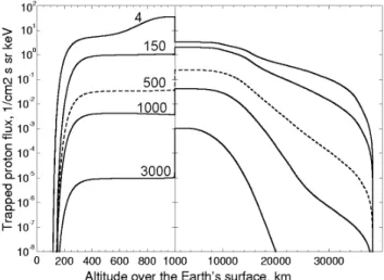
Figure 9 shows a flux of the re-ionized hydrogen ions calculated according to the equation 2. An abrupt changes in the curves at the altitude of 1000kmis a result of to the limitations of the atmospheric model used, which gives the gas concentrations only up to 1000km(see Fig. 3). The geocorona model used for the higher altitudes contains no date for the elements heavier than hydrogen. Due to that the result from 1000kmup to∼4000kmis not quite correct.
Figure 9. Dependence of the intensity of the re-ionized hydrogen ions (i.e. protons) versus altitude. The numbers next to the curves marks the ion energies. An abrupt bound of the simulated flux at the altitude of 1000kmis caused by incompleteness of the exo-spheric model used for the altitudes exceeding 1000km.
observed in that region where the intensity of the diffusive source of the inner radiation belt is already too low com-pared to the neutralization losses.
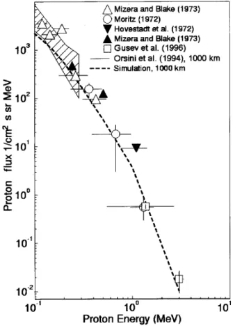
The results of the simulation are compared with experi-mental data in Fig. 10. The simulated flux agrees very well with experimental results including Orsini et al., [8]. To get the proton flux the neutral spectrum obtained in the latter in-side the radiation belt was multiplied by the factorD/P for the altitude of 1000km.
Figure 10. Comparison of the simulated result with experimental data.
4
Conclusion
We have numerically simulated the fluxes of the energetic neutral hydrogen atoms and quasi-trapped protons assum-ing their origin in charge-transfer reactions of the protons of the traditional radiation belt with constituencies of the exo-sphere and atmoexo-sphere. Standard models describing proton fluxes of the radiation belts, the atmospheric composition and the geocorona were used. It is shown that these pro-tons occupy a vast region of the magnetosphere comparable with that populated with the protons of the traditional radia-tion belt. The shape and the absolute values of the simulated quasi-trapped proton spectra agree well with all the set of the experimental results. That is one more confirmation of cor-rectness of the hypothesis of their origin and adequateness of the current atmospheric and magnetospheric models. The results presented here indicate to a potential of the quasi-trapped proton observations for monitoring global dynamics of the inner atmosphere.
Acknowledgments
This work has been supported by grants from CNPq (A.A. Gusev) and FAPERGS (G.I. Pugacheva). The model AP8 was obtained from the web pages of NASA’s National Space Science Data Center.
References
[1] J. Moritz, Z. Geophys.38, 701 (1972).
[2] D. Hovestadt, B. Hausler, and M, Scholer, Phys. Rev. Lett.
28, 1340 (1972).
[3] P. F. Mizera, and J. B. Blake, J. Geophys. Res, 78, 1058 (1973).
[4] H. D. Voss and L. G. Smith, COSPAR Adv. Space Explor.8, 131 (1979).
[5] T. G. Guzik, M. A. Miah, J. W.Mitchel, and J.P. Wefel, J. Geophys. Res,94, 145 (1989).
[6] A. A. Gusev, T. Kohno, W. N. Spjeldvik, I. M. Martin, G. I. Pugacheva, and Turtelli Jr., J. Geophys. Res, 101, 19659 (1996).
[7] M. E. Greenspan, G. M. Mason, and J. E. Mazur, J. Geophys. Res,104, 19911 (1999).
[8] S. Orsini, I.A. Daglis, M. Candidi, K.C. Hsieh, S. Livi, and Wilken, J. Geophys.Res,99, 13489 (1994).
[9] G. Gloeckler, F. M. Ipavich, W. Studemann., B. Wilken, D. C. Hamilton, G. Kremser, D. Hovestadt, F. Gliem, R. A. Lundgren, W. Rieck, E. O. Tums, J. C. Cain, L. S. Masung, W. Weiss, and P. Winterhof charge-energy-mass (CHEM) spectrometer for 0.3-300 keV/e ions on the AMPTE/CCE, IEEE Transactions on geoscience and remote sensing, 23, 234 (1985).
[10] B. A. Tinsley, J. Atmos. Terr. Phys. 43, 617 (1981).
[11] B. A. Tinsley, R. P. Rhorbaugh, H. Rassoul, E. S. Barker, A. L. Cochran, W. D. Cochran, B. J. Wills, D. W. Wills, and D. Slater, Geophys. Res. Lett.11, 572 (1984).
[12] B.A. Tinsley, R. P. Rhorbaugh, H. Rassoul, Y. Sahai, N.R. Teixeira, and D. Slater, J. Geophys. Res.91, 11257 (1986a). [13] B. A. Tinsley, R. R. Hodges, Jr., and R. P. Rhorbaugh, H.
Rassoul, J. Geophys. Res.91, 13631 (1996b).
[14] W. Bernstein, G.T. Inouye, N.L. Sanders, and R. L. Wax, J. Geophys. Res.74, 3601 (1969).
[15] Roederer J. G.,Dynamics of geomagnetically trapped radia-tion, Springer-Verlag, Heidelberg-New York, (1970). [16] A. E. Hedin, J. Geophys. Res.96, 1159 (1991).
[17] R. L. Rairden., L. A. Frank, and J. D. Craven, J. Geophys. Res,91, 13613 (1986).
[18] J. W. Chamberlen, Planet Space Sci,11, 901 (1963). [19] S. K. Allison, Rev. Mod. Phys.30, 1137 (1958).
[20] K. L. Riesselman, W. Anderson, L. Durand, and C. J. Ander-son, Phys. Rev. A,43, 5934 (1991).