An inkling of the relation between the monofractality of temperatures and pressure anomalies

(1)

NPGD

2, 1339–1353, 2015

Monofractality of temperatures

vs. pressure anomalies

A. Deliège and S. Nicolay

Title Page

Abstract Introduction

Conclusions References

Tables Figures

◭ ◮

Back Close

Full Screen / Esc

Printer-friendly Version Interactive Discussion

Discussion

P

a

per

|

Discussion

P

a

per

|

Discussion

P

a

per

|

Discussion

P

a

per

|

Nonlin. Processes Geophys. Discuss., 2, 1339–1353, 2015 www.nonlin-processes-geophys-discuss.net/2/1339/2015/ doi:10.5194/npgd-2-1339-2015

This discussion paper is/has been under review for the journal Nonlinear Processes in Geophysics (NPG). Please refer to the corresponding final paper in NPG if available.

An inkling of the relation between the

monofractality of temperatures and

pressure anomalies

A. Deliège and S. Nicolay

University of Liège, Institut de Mathématiques, Quartier Polytech 1, Allée de la Découverte 12, 4000 Liège, Belgium

Received: 28 April 2015 – Accepted: 26 June 2015 – Published: 18 August 2015 Correspondence to: A. Deliège ([email protected])

(2)

NPGD

2, 1339–1353, 2015

Title Page

Tables Figures

◭ ◮

Back Close

Full Screen / Esc

Discussion

P

a

per

|

Discussion

P

a

per

|

Discussion

P

a

per

|

Discussion

P

a

per

|

Abstract

We use the discrete “wavelet transform microscope” to study the monofractal nature of surface air temperature signals of weather stations spread across Europe. This method reveals that the information obtained in this way is richer than previous works studying long range correlations in meteorological stations: the approach presented

5

here allows to bind the Hölder exponents with the standard deviation of surface pressure anomalies, while such a link does not appear with methods previously carried out.

1 Introduction

Fractals have been extensively used in geosciences (see e.g. Arneodo et al., 2002;

10

Blenkinsop et al., 2000; Lovejoy and Schertzer, 1995, 2013; Schertzer and Lovejoy, 1991; Schertzer et al., 2002; Tessier et al., 1993). The aim of this paper is to show that the monofractal nature of raw temperature signals is related to surface pressure anomalies. For that purpose, we first present the wavelet leaders method (WLM) as a tool for providing a multifractal formalism, which is a more recent version of the

15

wavelet transform modulus maxima used in Arneodo et al. (2002, 1995). This method has already proven to be well-suited to study fractal objects (Abry et al., 2010; Jaffard, 2004; Jaffard and Nicolay, 2009; Lashermes et al., 2008; Wendt et al., 2009). We then use this wavelet-based approach to obtain results about the monofractality of the surface air temperature signals from a mathematical point of view. Finally, we show

20

that the fluctuation of the monofractal exponent observed from one station to another is bonded to surface pressure anomalies. Such a relation is not observed with methods usually associated with monofractal studies previously used on these signals (Bunde and Havlin, 2002). A possible explanation could be found in the fact that the WLM can be applied to the “raw signal”.

25

(3)

NPGD

2, 1339–1353, 2015

Title Page

Tables Figures

◭ ◮

Back Close

Full Screen / Esc

Discussion

P

a

per

|

Discussion

P

a

per

|

Discussion

P

a

per

|

Discussion

P

a

per

|

2 On the monofractal nature of temperature signals

Let us first recall the WLM. The discrete wavelet transform (WT) allows to decompose a signal using a single oscillating windowψcalled a wavelet (Daubechies, 1992; Mallat, 1999; Meyer, 1992). The WT of a functionf is defined as

Wψ[f](j,k)=2−j Z

f(x)ψ(2−jx+k)dx,

5

wherek is the space parameter andj the scale parameter (both take integer values). WT is well adapted to study the irregularities off, even if they are masked by a smooth behavior. Iff has, at a given pointx0, a local Hölder exponenth(x0), in the sense that

|f(x)−Px₀(x)| ∼ |x−x0| h(x₀)

around x0, where Px₀ is a polynomial, then with the right choice ofψ, one hasW_ψ[f](j,k)∼2−j h(x0)_{for the indices}_k _{such that 2}−j_x_−k_{is close to}

10

x0(Jaffard, 2004; Jaffard and Nicolay, 2009). The WLM is somehow a transposition of the wavelet transform modulus maxima (WTMM) to the discrete setting with a stronger theoretical background (Arneodo et al., 2002, 1995; Jaffard, 2004; Jaffard et al., 2006; Jaffard and Nicolay, 2009). Mimicking the box-counting technique, one investigates the scaling behavior of the partition function

15

S(q,j)₌2jX k

(sup j′_≥_j|Wψ

[f](j′,k)|)q,

through the function

ω(q)=lim_j_→+∞log(S(q,j)) log 2−j ,

whereqis a real parameter. In this framework, performing a Legendre transform of ω

gives a good approximation of the spectrum of singularities, defined as the Hausdor_ff

20

(4)

NPGD

2, 1339–1353, 2015

Title Page

Tables Figures

◭ ◮

Back Close

Full Screen / Esc

Discussion

P

a

per

|

Discussion

P

a

per

|

Discussion

P

a

per

|

Discussion

P

a

per

|

spectrum of singularities is the function that “counts”, for a given Hölder exponenth, the number of points havinghas Hölder exponent. Monofractal functions, i.e. functions with a constant Hölder exponent h(x0)=H are characterized by a linear function ω:

H=∂ω/∂q, which is equivalent to a spectrum of singularities reduced to the point (H, 1). On the contrary, a nonlinear ω curve is the signature of functions displaying

5

a multifractal behavior; in this case,his not constant anymore and thus may fluctuate from one point to another. Let us note that the wavelet used in this work is the second order Daubechies wavelet (Daubechies, 1992), but the results remain unchanged with higher orders.

In order to confirm that the analyzed signals are monofractal, we used the “surrogate

10

data method” (see Small et al., 2001; Theiler et al., 1992, for details). We first perform a Fourier transform of the data. Then, we randomize the Fourier phases but preserve the amplitudes and finally perform an inverse Fourier transform to create the surrogate series. Such a surrogate series has thus the same Fourier spectrum as the original data.

15

Since the Fourier spectrum is preserved with the surrogate procedure, the spectrum of singularities of a monofractal signal is not a_ffected either (Daubechies, 1992; Mallat, 1999). On the other hand, if the signal is multifractal, the regularity from one point to another is modified in the surrogate data and there is thus no reason for the spectrum of singularities to be preserved. In order to illustrate this fact, we performed a test on

20

two functions. The first is the well-known Weierstraß function defined as

f(x)=

+∞

X

j=1

2−jcos(4jx).

This function is monofractal with Hölder exponent 0.5 (see Nicolay, 2006, for details). The second one is the Lebesgue–Davenport function defined as

f(x)=1

2+

+∞

X

n=0

a_n{2nx}

25

(5)

NPGD

2, 1339–1353, 2015

Title Page

Tables Figures

◭ ◮

Back Close

Full Screen / Esc

Discussion

P

a

per

|

Discussion

P

a

per

|

Discussion

P

a

per

|

Discussion

P

a

per

|

witha_2n=2−nanda_2n₊1=−2− n−1

and where{x}is the sawtooth wave:{x}=x− ⌊x⌋ −

0.5 ifx is not an integer and {x}=0 else. It can be shown (see Jaffard and Nicolay, 2009, 2010) that the Lebesgue–Davenport function is multifractal with a spectrum of singularities given byd(h)=2hwith 0≤h≤0.5. The regularity of these two functions was studied with the WLM and the results are represented in Fig. 1. One can clearly

5

see that the spectrum of singularities of a monofractal function is blind to the surrogate procedure, whereas a multifractal function and its surrogate display completely different spectra.

We applied the WLM on daily mean surface air temperature data collected from the European Climate Assessment and Dataset (http://ecad.eu) and computed as the

10

mean between the daily minimum and daily maximum temperatures. In order to get homogeneous signals, we limited our study to temperature series with at least 50 years of data between 1951 and 2003 spread across Europe between 36◦ (Southern Spain, Italy, Greece) and 55◦ of latitude (Northern Ireland, Germany) and −10◦ (Western Ireland, Portugal) and 40◦of longitude (Eastern Ukraine). By doing so, we were able to

15

select 115 weather stations uniformly dispersed across the selected area (see Fig. 2). For the purpose of reducing the noise, the data f(t) were replaced by their temperature profilesPt

u=1f(u).

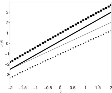
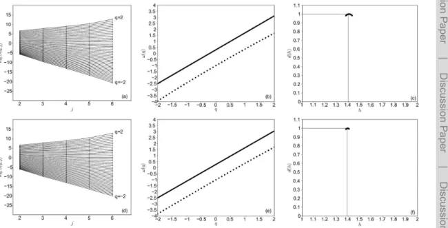
As shown in Fig. 3, one can see that the air temperature signal of Rome displays a monofractal nature: the function ω is clearly linear (coefficient of determination

20

R2>0.995). Also, the associated spectrum of singularities is blind to the surrogate procedure, which confirms the monofractal nature of the signal (see Fig. 4).

Such an observation holds for all the stations, which indicates that air temperature signals are monofractal. However, the value of the Hölder exponent varies from one station to another as illustrated in Fig. 3 with the stations of Rome and Armagh

25

(6)

NPGD

2, 1339–1353, 2015

Title Page

Tables Figures

◭ ◮

Back Close

Full Screen / Esc

Discussion

P

a

per

|

Discussion

P

a

per

|

Discussion

P

a

per

|

Discussion

P

a

per

|

These usual values (about 0.65) are recovered when the seasonal trends are removed (data not shown). Let us also remark that other methods (Sν, see Kleyntssens et al., 2015, WTMM, see Arneodo et al., 2002, 1995) based on the raw data give similar results.

Studies about LRC in air temperature data have been carried out using the DFA

5

(detrended fluctuation analysis, see e.g. Bunde and Havlin, 2002; Koscielny-Bunde et al., 1998). From a methodological point of view, this method displays some similarities with the WLM. However, the DFA is concerned with LRC, not with Hölder exponents. Moreover, the DFA requires the seasonal trends to be removed whereas the WLM does not; both methods are then used with the cumulative sum of the signals.

10

Therefore, the DFA studies LRC within the summed detrended signal while the WLM allows to compute the Hölder exponent of the summed raw signal.

3 Relation with pressure anomalies: a statistical approach

A natural question arising is whether or not the observed Hölder exponents can be bond to some climate index. A natural choice is to try to link the surface

15

pressure anomalies with the Hölder exponents in the following sense: can we recover the correlation structure observed in the pressure anomalies field from the spatial repartition of the Hölder exponents? Moreover, can such a structure be recovered with the DFA? To answer these questions, the map of Europe is gridded into roughly 200 km2pixels. We compare the map of the inverses of standard deviations of surface

20

pressure anomalies from the NCEP-NCAR Reanalysis Project (http://www.esrl.noaa. gov/) with the map made of the measured Hölder exponents. From a statistical point of view, we try to show that the null hypothesis, stating that the two maps are mutually independent, can be rejected. To do so, for both maps, each pixel (corresponding to an anomaly or a Hölder exponent) is normalized in order to obtain values between 0

25

and 1. The likeness between these maps is defined as the distance between them (considered as matrices):

(7)

NPGD

2, 1339–1353, 2015

Title Page

Tables Figures

◭ ◮

Back Close

Full Screen / Esc

Discussion

P

a

per

|

Discussion

P

a

per

|

Discussion

P

a

per

|

Discussion

P

a

per

|

d=

s X

i,j

(xi,j−x′_i,j)2,

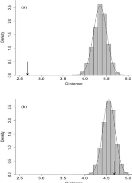
wherexi,j is a pixel of the first map,xi′,j is the corresponding pixel of the second map and where the sum is taken over all pixels. In this case, the likeness between the maps isd1=2.68. In order to check if these maps are akin, we use a standard Monte–Carlo method: the “Hölder map” is randomly shu_ffled 10 000 times. For each realization, the

5

distance with the original anomalies map is computed in order to get a distribution of these random distances. In this way, one can look whered1 lies in the distribution of the distances, and one can associate ap value to this particular distance d1. Based on the 10 000 observations, the probability 1−pto have a randomly shuffled map with a distance smaller thand1is lower than 10−

4

, which shows that the null hypothesis can

10

be rejected with a high confidence level (see Fig. 5a). In other words, the higher the standard deviation of pressure anomalies, the lower the Hölder exponents.

In order to show that the DFA method carried out in Koscielny-Bunde et al. (1998) does not display analogue correlation structures, we perform the same simulation but with a map where the Hölder exponents obtained with the WLM are replaced with the

15

values obtained with the DFA. In this case, the distanced2between this “DFA map” and the anomalies map is 4.68, and the probability that the distance between a randomly shuffled DFA map and the anomalies map be smaller thand2is 1−p=0.8. This shows that the DFA map cannot be considered as correlated to pressure anomalies (see Fig. 5b). One can thus conclude that the values obtained via the DFA have no obvious

20

(8)

NPGD

2, 1339–1353, 2015

Title Page

Tables Figures

◭ ◮

Back Close

Full Screen / Esc

Discussion

P

a

per

|

Discussion

P

a

per

|

Discussion

P

a

per

|

Discussion

P

a

per

|

4 Conclusions

As a conclusion, one can say that the Hölder exponents obtained here with the WLM reflect in some way the climate variability of the stations associated to the data: standard deviations of pressure anomalies and Hölder exponents are anti-correlated. Such a result does not appear with methods that first require the seasonal variations

5

to be removed. Future work consists in investigating the possible relation between the Hölder exponents of the stations and their climate type, which could bring new information about the regularity of temperatures.

Acknowledgements. We acknowledge the data providers in the ECA&D project. Klein Tank, A. M. G. and Coauthors, 2002. Daily dataset of 20th-century surface air temperature and

10

precipitation series for the European Climate Assessment, Int. J. of Climatol., 22, 1441–1453. Data and metadata available at http://www.ecad.eu. We also acknowledge the data providers in the NCEP/NCAR Reanalysis Project (GHCN Gridded V2 data were provided by the NOAA-OAR-ESRL PSD, Boulder, Colorado, USA, from their Web site at http://www.esrl.noaa.gov/).

References

15

Abry, P., Wendt, H., Jaffard, S., Helgason, H., Goncalves, P., Pereira, E., Charib, C., Gaucherand, P., and Doret, M.: Methodology for multifractal analysis of heart rate variability: from LF/HF ratio to wavelet leaders, in: Nonlinear Dynamic Analysis of Biomedical Signals EMBC conference (IEEE Engineering in Medicine and Biology Conferences), 31 Augst 2010–4 September 2010, Buenos Aires, 106–109, 2010. 1340

20

Arneodo, A., Bacry, E., and Muzy, J.: The thermodynamics of fractals revisited with wavelets, Physica A, 213, 232–275, 1995. 1340, 1341, 1344

Arneodo, A., Audit, B., Decoster, N., Muzy, J.-F., and Vaillant, C.: Wavelet Based Multifractal 25 Formalism: Applications to DNA Sequences, Satellite Images of the Cloud Structure, and Stock Market Data, in: The Science of Disasters: Climate Disruptions, Heart Attacks, and

25

Market Crashes, Springer, Berlin, Germany, 27–105, 2002. 1340, 1341, 1344

Blenkinsop, T., Kruhl, J., and Kupkova, M.: Fractals and Dynamic Systems in Geoscience, Birkhauser, Basel, Switzerland, 2000. 1340

(9)

NPGD

2, 1339–1353, 2015

Title Page

Tables Figures

◭ ◮

Back Close

Full Screen / Esc

Discussion

P

a

per

|

Discussion

P

a

per

|

Discussion

P

a

per

|

Discussion

P

a

per

|

Bunde, A. and Havlin, S.: Power-law persistence in the atmosphere and in the oceans, Physica A, 314, 15–24, 2002. 1340, 1344

Daubechies, I.: Ten Lectures on Wavelets, SIAM, Philadelphia, USA, 1992. 1341, 1342, 1345 Jaffard, S.: Wavelet techniques in multifractal analysis, P. Symp. Pure Math., 72, 91–152, 2004.

1340, 1341

5

Jaffard, S. and Nicolay, S.: Pointwise smoothness of space-filling functions, Appl. Comput. Harmon. A., 26, 181–199, 2009. 1340, 1341, 1343

Jaffard, S. and Nicolay, S.: Space-filling functions and Davenport series, in: Recent Developments in Fractals and Related Fields, Birkhauser, New York, USA, 19–34, 2010. 1343

10

Jaffard, S., Lashermes, B., and Abry, P.: Wavelet leaders in multifractal analysis, in: Wavelet Analysis and Applications, Birkauser, Basel, Switzerland, 201–246, 2006. 1341

Kleyntssens, T., Esser, C., and Nicolay, S.: A multifractal formalism based on theSν spaces: from theory to practice, in review, 2015. 1344

Koscielny-Bunde, E., Bunde, A., Havlin, S., Roman, H., Goldreich, Y., and Schellnhuber, H.-J.:

15

Indication of a universal persistence law governing atmospheric variability, Phys. Rev. Lett., 81, 729–732, 1998. 1343, 1344, 1345

Lashermes, B., Roux, S., Abry, P., and Jaffard, S.: Comprehensive multifractal analysis of turbulent velocity using wavelet leaders, Eur. Phys. J. B, 61, 201–215, 2008. 1340

Lovejoy, S. and Schertzer, D.: Multifractals and rain, in: New Uncertainty Concepts in Hydrology

20

and Water Resources, Cambridge University Press, New York, USA, 61–103, 1995. 1340 Lovejoy, S. and Schertzer, D.: The Weather and Climate: Emergent Laws and Multifractal

Cascades, Cambridge University Press, Cambridge, UK, 2013. 1340

Mallat, S.: A Wavelet Tour of Signal Processing, Academic Press, New York, USA, 1999. 1341, 1342

25

Meyer, Y.: Wavelets and Operators, Cambridge University Press, Cambridge, UK, 1992. 1341 Nicolay, S.: Analyse de Sequences ADN par la Transformee en ondelettes: extraction

d’informations structurelles, dynamiques et fonctionnelles, PhD thesis, Universite de Liege and Ecole Normale Superieure de Lyon, 2006. 1342

Schertzer, D. and Lovejoy, S.: Non-Linear Variability in Geophysics: Scaling and fractals,

30

(10)

NPGD

2, 1339–1353, 2015

Title Page

Tables Figures

◭ ◮

Back Close

Full Screen / Esc

Discussion

P

a

per

|

Discussion

P

a

per

|

Discussion

P

a

per

|

Discussion

P

a

per

|

Schertzer, D., Lovejoy, S., and Hubert, P.: An Introduction to Stochastic Multifractal Fields, in: ISFMA Symposium on Environmental Science and Engineering with related Mathematical Problems, edited by: Ern, A. and Liu, W., Beijing, China, 106–179, 2002. 1340

Small, M., Judd, K., and Mees, A.: Testing time series for nonlinearity, Stat. Comput., 11, 257– 268, 2001. 1342

5

Tessier, Y., Lovejoy, S., and Schertzer, D.: Universal multifractals: theory and observations for rain and clouds, J. Appl. Meteorol., 32, 223–250, 1993. 1340

Theiler, J., Eubank, S., Longtin, A., Galdrikian, B., and Farmer, J. D.: Testing for nonlinearity in time series: the method of surrogate data, Physica D, 58, 77–94, 1992. 1342

Wendt, H., Abry, P., Jaffard, S., Ji, H., and Shen, Z.: Wavelet leader multifractal analysis for

10

texture classification, in: Proc IEEE conf. ICIP, 7–10 November 2009, Cairo, Egypt, 3829– 3832, 2009. 1340

(11)

NPGD

2, 1339–1353, 2015

Title Page

Tables Figures

◭ ◮

Back Close

Full Screen / Esc

Discussion

P

a

per

|

Discussion

P

a

per

|

Discussion

P

a

per

|

Discussion

P

a

per

|

Figure 1. First column: (a) Weierstraß function, (d) a surrogate of the Weierstraß function,

(12)

NPGD

2, 1339–1353, 2015

Title Page

Tables Figures

◭ ◮

Back Close

Full Screen / Esc

Discussion

P

a

per

|

Discussion

P

a

per

|

Discussion

P

a

per

|

Discussion

P

a

per

|

Figure 2.Localization of the studied weather stations across Europe.

(13)

NPGD

2, 1339–1353, 2015

Title Page

Tables Figures

◭ ◮

Back Close

Full Screen / Esc

Discussion

P

a

per

|

Discussion

P

a

per

|

Discussion

P

a

per

|

Discussion

P

a

per

|

0

−2 −1.5 −1 −0.5 0.5 1 1.5 2

−3 −2 −1 0 1 2 3

(14)

NPGD

2, 1339–1353, 2015

Title Page

Tables Figures

◭ ◮

Back Close

Full Screen / Esc

Discussion

P

a

per

|

Discussion

P

a

per

|

Discussion

P

a

per

|

Discussion

P

a

per

|

Figure 4. (a)The function logS(q,j) vs.j for qranging from−2 to 2 (from bottom to top) by step of 0.1 for Rome. For a fixedq, the slope of the linear regression over logS(q,j) gives the value ofω(q) (seeb).(b) Function ωfor Rome (dots). The thick straight line represents the linear regression line ofωand shows thatωis clearly linear, which implies that the signal is monofractal with Hölder exponent given by the slope of the regression line: 1.4.(c)Associated spectrum of singularities. Graphs(d–f)represent the corresponding figures for the surrogate signal. One can clearly see that the spectrum of singularities is not affected by the surrogate procedure, which confirms that the signal is monofractal.

(15)

NPGD

2, 1339–1353, 2015

Title Page

Tables Figures

◭ ◮

Back Close

Full Screen / Esc

Discussion

P

a

per

|

Discussion

P

a

per

|

Discussion

P

a

per

|

Discussion

P

a

per

|

Figure 5. (a) (resp. b): histogram of the distances between the randomly shuffled Hölder maps (resp. randomly shuffled DFA maps) and the inverses of standard deviations of pressure anomalies map. The curves represent the theoretical Gaussian distributions based on the mean and the standard deviation of the measured distances. The arrow indicates the distancesd₁