Article
J. Braz. Chem. Soc., Vol. 25, No. 2, 208-218, 2014. Printed in Brazil - ©2014 Sociedade Brasileira de Química 0103 - 5053 $6.00+0.00
A
*e-mail: [email protected]
Application of a Multivariate Exploratory Analysis Technique in the
Study of Dissolved Organic Matter and Metal Ions in Waters from the
Eastern Quadrilátero Ferrífero, Brazil
Erik S. J. Gontijo,*, a Francysmary S. D. Oliveira,a Mariana L. Fernandes,a
Gilmare A. da Silva,b Hubert M. P. Roesera and Kurt Friesec
aDepartment of Environmental Engineering and bDepartment of Chemistry, Federal University of Ouro Preto (UFOP), Morro do Cruzeiro, S/N, 35400-000 Ouro Preto-MG, Brazil
cUFZ - Department Lake Research, Helmholtz-Centre for Environmental Research, Brückstraße 3a, 39114 Magdeburg, Germany
Amostras de água foram coletadas em 10 pontos em trechos do leste do Quadrilátero Ferrífero (QF), que é uma região mineira situada no sudeste do Brasil. Os objetivos deste estudo foram encontrar possíveis relações entre carbono orgânico dissolvido (COD), metais e outros parâmetros físico-químicos medidos utilizando a rede neural de Kohonen como ferramenta para analisar esses
dados geoquímicos multivariados na área estudada. As análises físico-químicas foram feitas in situ
e em laboratório, onde as concentrações de COD e vários íons metálicos foram determinadas. A rede de Kohonen permitiu a visualização e interpretação mais amigáveis dos dados, além de definir relações entre eles. Assim, para os dados analisados, foi verificada relação entre COD e Fe e um possível efeito da sazonalidade na distribuição das amostras. Possíveis evidências litológicas puderam ser detectadas pela análise exploratória, especialmente se considerados os elementos Ca, Mg, Mn e Sr.
Water samples were collected at 10 points in parts of the eastern Quadrilátero Ferrífero (QF), located in a mining region in the southeast of Brazil. The aims of this study were to find possible relationships among dissolved organic carbon (DOC), metals and other parameters measured in the region studied and evaluate the Kohonen neural network as a tool to analyse this geochemical
multivariate data set. Physico-chemical analyses were performed in situ and in the laboratory,
where concentrations of DOC and a suite of metal ions were determined. The Kohonen neural network allowed an easier visualisation and interpretation of the results and helped to define the relationships among them. In this way, a relationship between DOC and Fe and a possible effect of seasonality on the distribution of the samples were indicated. Signs of lithology were detected in the analyses, especially considering the elements Ca, Mg, Mn and Sr.
Keywords: Quadrilátero Ferrífero - Brazil, dissolved organic carbon, Kohonen neural network, environmental geochemistry
Introduction
The Quadrilátero Ferrífero (QF) is a geological structure in the southeast of Brazil that is worldwide known for its mineral deposits.1 It covers an area of approximately
7000 km2 in the Brazilian state of Minas Gerais and
constitutes a southern extension of the Espinhaço Mountain Range, in the south-eastern part of the São Francisco Craton.1,2 In this region, iron and gold are the dominant
products in the mining area, along with aluminium and topaz. It is remarkable that the QF has become the most important gold producer in the late seventeenth century, with a total production that probably exceeded 1300 t in history.3,4
metasediments, which tends to release major elements such as Na, K, Ca, Mg, Mn and Fe, and trace elements such as Ni, Cr, Co and V. The Minas Supergroup comprises Proterozoic metasediments, which are source of Fe, Mn, Ca and Mg. The Itacolomi Group consists predominantly of quartzitic rocks.1,2
One of the consequences of mining and associated activities is the alteration of the elements cycle in the environment, which influences the availability of metals to organisms. This is exactly what occurs along the Quadrilátero Ferrífero, where the exploitation of iron ore, for instance, acts as an important source of major elements such as Fe and Mn, and trace metals. In addition, it is important to consider that gold mining can release As and Cu, which are present in minerals such as iron sulfides (pyrite, FeS2), copper sulfides (chalcopyrite, CuFeS2) and
arsenic sulfides (arsenopyrite, FeAsS), often in paragenesis with gold.2,5
In the aquatic environment, the dissolved organic carbon (DOC) is considered a regulator of biotic and abiotic processes. It is operationally defined as the fraction of organic material that passes through a 0.45 µm filter.6
The dissolved organic matter is a vital resource that will affect food webs either directly, by its use via organisms, or indirectly via mechanisms such as turbidity, pH and contaminant transportation.6,7 The DOC has the ability to
decrease the toxicity of many metals while it reduces the availability of these elements to organisms by means of chemical bonds. This has particular importance given that the QF is a region rich in minerals and suffers from the impacts caused by mining. The variety of minerals is able to release a range of elements in the water bodies where they interact with dissolved organic matter, especially humic substances (HS), which constitute about 80% of the DOC in natural waters.8 Considering that the concentration of
dissolved metal ions and organic material can influence the formation of metal-HS complexes, it is important to identify possible interactions between these chemicals and the organic material.9
Due to the large number of variables generally analysed in environmental geochemistry studies, techniques of exploratory data analysis have been shown to be effective in identifying patterns in a group of data, facilitating the interpretation of results.10 An example of a tool developed
for multivariate exploratory analysis is the Kohonen neural network (Self-Organising Maps, SOM), which is an artificial intelligence technique that has the ability to project high dimensional data in a space of lower dimension, without loss of the original information. It was developed by Teuvo Kohonen (Finland) and has a close relationship with the organisation of the cerebral cortex.11
An important advantage of this tool is the ease of viewing and interpreting the data.12 To summarise, the Kohonen
neural network comprises self-organising maps, which are formed by neurons arranged in a two-dimensional array. In fact, this is one of the main advantages of the Kohonen neural network, explicitly, the possibility of getting all data information (relationship between samples, variables and the influence of variables in samples) in a two-dimensional array. In addition, this characteristic is also one of the main advantages of this method compared with other exploratory approaches, such as Principal Component Analysis (PCA), where in most cases it is necessary to work with multidimensional spaces (more than two-dimensional arrays) provided by the principal components (PC). Kohonen structures with higher dimensions are also possible, but are less common.11-13
In the Kohonen neural network, it is assumed that all the samples placed at the same neuron are similar to each other according to the aspect analysed. Another important attribute of this technique is the formation of clusters of samples that are considered to possess the same characteristics, because of its location in nearby neurons (neighbouring neurons).12
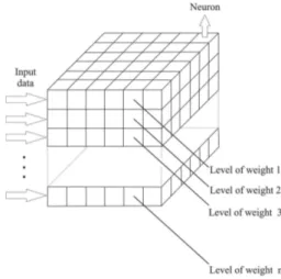
A picture representing the typical architecture of the Kohonen neural network is shown in Figure 1, where the neurons are represented by columns, or tubes arranged inside a box. In this type of representation, if a specific input data has n samples, n input vectors x will be obtained. These vectors x may be absorbance values of a spectrum, peaks of a chromatogram or intensity values of different physico-chemical parameters of the water quality. It is important to note that the dimensionality of the vector is dependent upon the number of variables in the data, which means that the amount of weights of each neuron (w) will correspond to the number of vector elements of the input data.12
Figure 1. Representation of the typical architecture of the Kohonen
The Kohonen network was not performed before in the study of metal ions and DOC in surface waters of Quadrilátero Ferrífero. Furthermore, this kind of study in the specific evaluated area was not found in scientific literature yet. Considering similar studies worldwide, it is possible to find successful applications of the SOM technique in multivariate data analysis.13,14 Notably, the
Kohonen network has also been successfully used in fields ranging from ecology until the evaluation of the performance of a wastewater treatment plan.15-17
The present work was an initial study that aimed to investigate the levels of dissolved organic matter in some brown-coloured water bodies and its probable relationships with metal ions and other parameters measured in the eastern part of the QF. The application of a multivariate exploratory analysis for this kind of study in the region is an innovative to visualise the results and the relationships among samples and its variables in an easy and effective way
Experimental
Sampling and preliminary analyses
Ten sampling points were selected in upper Rio Doce River Basin based on the accessibility and on visual inspection of some water bodies. Areas with brown-coloured waters were preferable in this process because they could indicate higher levels of dissolved organic matter. The study area comprised parts of the eastern QF and is shown on the map in Figure S1 (Supplementary Information). The physico-chemical parameters pH, temperature (T), total dissolved solids (TDS), redox potential (ORP), resistivity (Resis), conductivity (Cond) and turbidity (Turb) were evaluated in situ using a multiparameter equipment (Ultrameter II, Myron L Company) and a turbidimeter (DM-TU Digimed) previously calibrated.
It is important to note that in the studied area, Cwa and Cwb climates occur.18,19 Both climates are characterised by
a dry winter. In the area where the Cwa climate occurs, the dry period is between April and September and the rainiest months are November and December. The areas where the Cwb climate occurs, the dry season is between May and August and the rainfalls are concentrated mainly between November and February. For this reason, more than one sampling at different times was performed for some points in order to evaluate possible influences of seasonality. However, there was a problem in one sampling of point 1 because the swamp was totally dry in one winter field trip. Consequently, it was not possible to collect water for analyses at that time. From the data available in the
literature,18,19 the dry season in this work was considered
between April and September and the rainy season between October and March.
About 1 L of water was collected in accessible areas close to the water bodies (banks or on bridges) for the determination of sulfate, chloride (Cl) and alkalinity (Alc). The samples were kept refrigerated until laboratory analyses. The methodology used was based on standard methods proposed by the American Public Health Association (APHA).20 About 40 mL of water was collected
for analyses of metals and about 20 mL for analyses of DOC. These samples were filtered through membranes of 0.45 µm and kept refrigerated at 4 ºC until analysis in the laboratory. As described by Grasshoff, Kremling and Ehrhardt,21 the storage of samples in plastic containers
can cause interference in the results of carbon analyses. Therefore, it was chosen to keep the waters collected in amber glass bottles to avoid any changes by means of light in the humic material. After filtering the samples for analysis of metals, they were acidified by adding 3-4 drops of concentrated HNO3 to keep the metals in solution. All
reagents used in this work were of analytical grade.
Metal analyses
The analyses of metals were performed in the Laboratory of Environmental Geochemistry (LGqA) at Federal University of Ouro Preto (UFOP). The metals were analysed by inductively coupled plasma optical emission spectrometry (ICP-OES Spectro / Ciros model CCD) in radial mode. Output power of the generator was 1250 W, the pumping rate was 2 mL min−1, the gas flow of the
plasma was 12 L min−1 and the gas flow of the nebulizer
was 0.90 L min−1. In all cases, argon was used as gas.
The calibration was performed in all cases using standard stock solutions with analytical purity grade and was evaluated by means of international reference material NIST 1643c. The elements determined were the major metals Al, Ca, Fe, K, Mg, Mn, Na and Ti; and the trace metals As, Ba, Be, Cd, Co, Cr, Cu, Li, Mo, Ni, P, Pb, S, Sc, Sr, V, Y and Zn.
DOC analyses
determination of the TDC, the samples were introduced into a combustion tube, which was filled with an oxidation catalyst and heated to 680 ºC. Thereby, all components of the TDC are converted into CO2, which is detected by a
cell of non-dispersive infrared (NDIR) in the end of the procedure.
The DIC was measured by the same equipment after acidification of the samples using HCl to a pH less than 3. At this point, all the carbonates were converted to CO2. At
the end of the process, all CO2 was volatilised by bubbling
air or nitrogen gas and detected by the NDIR cell.
Multivariate analyses
The technique used for exploratory analysis in this work was the Kohonen neural network. The aim of this method was to reduce the number of dimensions to be analysed and preserve the relevant original information in order to facilitate the observation and interpretation of the results. Some of the metal contents determined had to be excluded from Kohonen analysis because their values were below the limit of quantification (LOQ). Therefore, the data set was organised into a matrix of 16 samples (16 lines) and 19 variables (19 columns). The samples represent the sampling points and the variables represent pH, DOC, Cond, Alc, ORP, T, Turb, Resis, TDS, Cl, Ba, Ca, Fe, K, Mg, Mn, Na, S and Sr values.
Before processing the data by the SOM algorithm, the entire data set was autoscaled for all variables, which means that the variance of the variables were normalised and the averages calculated to zero. The scaling of the variables is of vital importance in the application of Kohonen network, because its algorithm uses the Euclidean metric to measure distances between vectors. If a variable has values ranging between 0 and 1000 and another variable has values ranging between 0 and 1, for instance, the first will virtually dominate the organisation of the map because of the large impact on the measurement of distances. Hence, in most cases it is recommended that the variables are equally important. The pre-processing of data ensures that all variables have the same level of importance, allowing users to assess the significance of all variables in the samples. Since the variables investigated in this work refer to different physical and chemical measurements, the scaling of the data becomes obligatory.12
The Kohonen maps were created and initialised linearly. In this process, the eigenvalues and eigenvectors of the data were calculated. Then, the weight vectors of the map have been initialised over the largest eigenvectors of the covariance matrix in agreement with the size of the map,
which is generally 2. The Kohonen neural network was trained with the data using the batch training algorithm, where the entire data set is presented to the map before any adjustment of weights is done. The neighbourhood function used in training was the Gaussian, the structure was hexagonal and shape of the map was planar.12
At the end of the process, a map was obtained that shows the grouping of the samples and the influence of the variables. The lighter colours in the neurons indicate higher values for that variable. The darker colours represent the lowest values for the same variable. It is important to mention that the neurons of the map of the variables were compared with the neurons of the map of groups of samples to evaluate which parameters are influencing a given sample. During the data training, architectures with several orders were tested (from 2 × 2 to 6 × 6) for evaluation of the groups of samples and it was chosen the architecture that had the best sample distribution in groups (which was more informative).
The software used to perform the multivariate analysis of Kohonen neural network was freely available on the internet.22
For comparison, a PCA analysis was also performed using the same set of data through the computing environment GNU Octave 3.6.4, freely available on the internet at page http://www.gnu.org/software/octave/; before data processing, the entire data set was autoscaled for all variables.
Results and Discussion
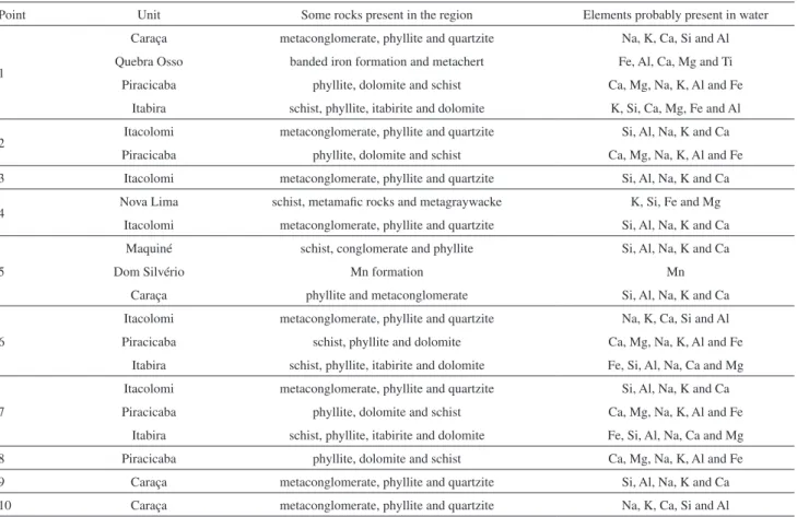
The location of the points, season and types of water bodies where the samplings were performed are shown in Table 1. From some lithological data and maps of the region, another table (Table 2) was created. This table shows the stratigraphic units, rocks in the region of the sampling points and some elements likely present in the waters sampled. It is important to consider that the points 9 and 10 were collected in an area of environmental protection (Private Reserve of Natural Heritage of Caraça). The results of the parameters measured in the field and in the laboratory are shown in Table 3.
Table 1. Location, type of water body and period of sampling in the studied area
Point Sample Coordinates Description (location) Type of water
body Season / Month / Year Latitude Longitude
1 S1A S 20o09’43.7’’ W 43o25’54.8’’ South plateau
(near Caraça Moutain Range) Swamp
Rainy / October / 2010
S1B Rainy / March / 2011
2
S2A
S 20o15’55.7’’ W 43o28’32.7’’ East of peak of Frazão Lake
Rainy / October / 2010
S2B Rainy / March / 2011
S2C Dry / August / 2011
3 S3A S 20o27’51.8’’ W 43o35’26.0’’ Itatiaia Mountain Range Swamp Rainy / November / 2010
S3B Dry / June / 2011
4 S4A S 20o29’49.5’’ W 43o36’55.6’’ Garcia River River Rainy / November / 2010
S4B Dry / June / 2011
5 S5 S 20o13’49.7’’ W 43o25’06.5’’ Ouro Fino Stream (near the village of
Bento Rodrigues) Stream Rainy / December / 2010
6 S6 S 20o16’33.9’’ W 43o25’51.3’’ Gualaxo do Norte River River Rainy / December / 2010
7 S7 S 20o16’50.0’’ W 43o26’25.5’’ Stream that flows into the Gualaxo do
Norte River Stream Rainy / December / 2010
8 S8 S 20o09’43.5’’ W 43o25’11.5’’ Brumado Stream Stream Rainy / March / 2011
9 S9A S 20o06’22.1’’ W 43o28’27.2’’ Cascatinha (Caraça Mountain Range) Stream Dry / May / 2011
S9B Dry / August / 2011
10 S10 S 20o05’52.9’’ W 43o29’23.4’’ Caraça Stream (Caraça Mountain Range) Stream Dry / May / 2011
Table 2. Stratigraphic units and lithology of the studied area; geological data from Dorr, Alkmim and Marshak23,24
Point Unit Some rocks present in the region Elements probably present in water
1
Caraça metaconglomerate, phyllite and quartzite Na, K, Ca, Si and Al
Quebra Osso banded iron formation and metachert Fe, Al, Ca, Mg and Ti
Piracicaba phyllite, dolomite and schist Ca, Mg, Na, K, Al and Fe
Itabira schist, phyllite, itabirite and dolomite K, Si, Ca, Mg, Fe and Al
2 Itacolomi metaconglomerate, phyllite and quartzite Si, Al, Na, K and Ca
Piracicaba phyllite, dolomite and schist Ca, Mg, Na, K, Al and Fe
3 Itacolomi metaconglomerate, phyllite and quartzite Si, Al, Na, K and Ca
4 Nova Lima schist, metamafic rocks and metagraywacke K, Si, Fe and Mg
Itacolomi metaconglomerate, phyllite and quartzite Si, Al, Na, K and Ca
5
Maquiné schist, conglomerate and phyllite Si, Al, Na, K and Ca
Dom Silvério Mn formation Mn
Caraça phyllite and metaconglomerate Si, Al, Na, K and Ca
6
Itacolomi metaconglomerate, phyllite and quartzite Na, K, Ca, Si and Al
Piracicaba schist, phyllite and dolomite Ca, Mg, Na, K, Al and Fe
Itabira schist, phyllite, itabirite and dolomite Fe, Si, Al, Na, Ca and Mg
7
Itacolomi metaconglomerate, phyllite and quartzite Si, Al, Na, K and Ca
Piracicaba phyllite, dolomite and schist Ca, Mg, Na, K, Al and Fe
Itabira schist, phyllite, itabirite and dolomite Fe, Si, Al, Na, Ca and Mg
8 Piracicaba phyllite, dolomite and schist Ca, Mg, Na, K, Al and Fe
9 Caraça metaconglomerate, phyllite and quartzite Si, Al, Na, K and Ca
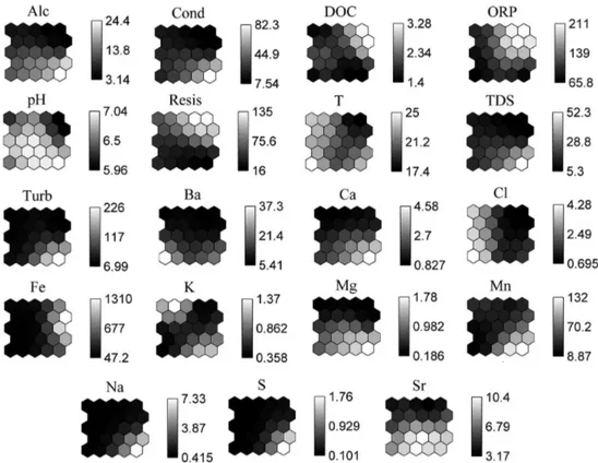
neuron or at neighbouring neurons form groups with similar characteristics. The map of the variables is shown in Figure 3, where the grayscale bars beside the maps indicate the intensity of each parameter evaluated. The lighter colours in these bars mean higher values and a higher importance in the formation of the groups for each variable.
It can be noted from Figure 2 and Figure 3 that K, temperature and Cl were the parameters responsible for making the samples S1B, S3A and S5 get closer and, therefore, form group I. These parameters were important because they had higher values for the samples of group I considering the data obtained in this exploratory study.
Although Cl was not measured for the sample S3A, the SOM algorithm estimates missing values during its training process. In this way, it is possible to infer about the behaviour of missing values.25
Potassium is a lithophile element that participates in the formation of silicates, feldspars and micas (biotite and muscovite), which are mineral constituents of rocks as gneisses and schist’s. Muscovite and biotite (that have K in their structure) are still part of the composition of quartzite rocks. Consequently, evaluating the lithotype of the region studied (Table 2) it can be noticed that the presence of K in the analyses is an indication of lithological contribution of this element for the waters in the studied area. The higher values detected for this element in group I may be explained by the fact that sampling of the samples S1B, S3A and S5 were performed in the rainy season (Table 1), where K is more leached by high precipitation.
In the environment, Cl can originate both from the weathering of rocks and by man’s influence via sewage discharges.26 In all samples, the concentrations of Cl were
very low, ranging from 0.50 mg L−1 to 4.66 mg L−1. As the
rocks of the region do not have Cl in their composition, probably the source of Cl can be atmospheric and/or from plants and animals (biogenic origin). It is important to note that the samples S1B and S8 may have some anthropogenic influence due to the proximity of a village (Santa Rita Durão). The breeding could influence the sample S2B because this type of activity is common in the region and
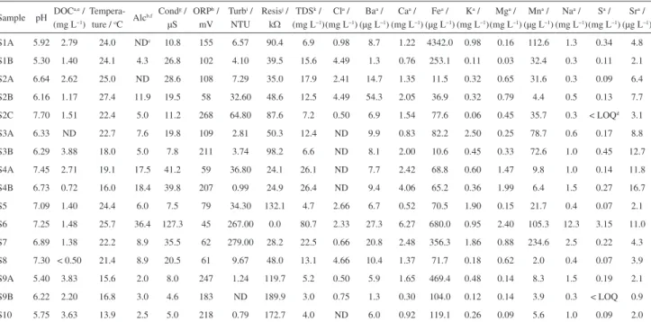
Table 3. Results of the physico-chemical parameters and metals analysed in natural waters of the upper Rio Doce River basin (Quadrilátero Ferrífero)
Sample pH DOC
a,e /
(mg L−1)
Tempera-ture / oC Alc
b,f Cond g /
µS ORPh /
mV Turbi /
NTU Resisj /
kΩ TDSk /
(mg L−1)
Cla /
(mg L−1)
Baa /
(µg L−1)
Caa /
(mg L−1)
Fea /
(µg L−1)
Ka /
(mg L−1)
Mga /
(mg L−1)
Mna /
(µg L−1)
Naa /
(mg L−1)
Sa /
(mg L−1)
Sra /
(µg L−1)
S1A 5.92 2.79 24.0 NDc 10.8 155 6.57 90.4 6.9 0.98 8.7 1.22 4342.0 0.98 0.16 112.6 1.3 0.34 4.8
S1B 5.30 1.40 24.1 4.3 26.8 102 4.10 39.5 15.6 4.49 1.3 0.76 253.1 0.11 0.03 32.4 0.3 0.11 2.1 S2A 6.64 2.62 25.0 ND 28.6 108 7.29 35.0 17.9 2.41 14.7 1.35 11.5 0.32 0.65 31.6 0.3 0.09 6.4 S2B 6.16 1.17 27.4 11.9 19.5 58 32.60 48.6 12.5 4.49 54.3 2.05 36.9 0.32 0.79 4.4 0.5 0.13 7.7 S2C 7.70 1.51 22.4 5.0 11.2 268 64.80 87.6 7.2 0.50 6.9 1.54 77.6 0.06 0.45 35.7 0.3 < LOQd 3.1
S3A 6.33 ND 22.7 7.6 19.8 109 2.81 50.3 12.4 ND 9.9 0.83 82.2 2.50 0.25 78.7 0.6 0.17 8.8 S3B 6.29 3.88 18.0 5.0 7.8 211 3.74 98.2 6.6 ND 8.1 2.00 10.6 0.45 0.33 72.6 1.0 0.45 12.7 S4A 7.45 2.71 19.1 17.5 41.2 59 36.80 24.1 26.1 ND 7.7 2.42 68.8 0.60 1.47 9.8 1.0 0.14 11.8 S4B 6.73 0.72 16.0 18.4 39.8 207 0.99 24.9 26.4 ND 9.4 4.06 65.2 0.36 1.99 6.4 1.5 0.27 16.7 S5 7.09 1.40 24.4 6.0 7.5 79 34.30 132.1 4.7 2.66 6.7 0.52 70.5 1.90 0.15 21.7 0.4 0.07 2.1 S6 7.25 1.48 25.7 36.4 127.3 45 267.00 0.0 80.7 2.33 27.3 6.27 680.0 0.95 2.40 105.3 12.3 3.15 11.0 S7 6.89 1.38 22.2 8.9 35.5 62 279.00 28.2 22.5 0.66 20.8 2.48 356.3 1.86 0.88 234.6 2.5 0.22 4.3 S8 7.30 < 0.50 21.4 8.9 20.5 61 9.67 48.0 13.1 4.66 10.4 1.37 71.7 0.18 0.62 2.0 0.4 0.07 3.9 S9A 5.40 3.83 15.6 2.0 8.0 247 1.24 119.7 5.2 0.50 5.9 1.65 469.4 0.48 0.14 8.3 1.5 0.19 2.1 S9B 6.22 2.20 16.8 3.0 4.6 183 ND 189.9 3.0 0.75 1.3 0.30 104.0 0.12 0.14 3.9 0.3 < LOQ 0.9 S10 5.75 3.63 13.9 2.5 5.0 218 0.79 172.7 4.0 ND 6.0 0.92 119.1 0.26 0.09 5.6 1.0 0.09 2.0
aStandard deviation calculated by replicate analyses was less than 10%; bGiven in mg CaCO
3 L−1; cND: Not determined; dLOQ: Limit of quantification; eDOC: dissolved organic
carbon; fAlc: alkalinity; gCond: conductivity; hORP: redox potential; iTurb: turbidity; jResis: resistivity; kTDS: total dissolved solids.
Figure 2. Map of groups of samples (natural waters) obtained by Kohonen
it could be seen during the field trips. These three points were the ones with the highest concentrations of Cl, with values above 4 mg L−1.
The summer in the southern hemisphere (December to March) corresponds to the period where higher volumes of precipitation are recorded considering the studied area.19
Consequently, Cl and K can be more leached by water from rainfalls and showed higher concentrations. This explains higher values in group I along with temperature. The second sampling of point 3 (S3B) plots in group II because the sampling was done in the dry season (June 2011, Table 1). From Figure 3, it can be noticed that the variables DOC and Fe indicated higher concentrations at neurons in the same location. These higher values influenced the positions of the samples in group II and suggest that Fe has positive relationship with DOC considering the samples analysed in this paper. This observation could indicate a complexation between these variables, since Fe can effectively bind organic matter, especially humic substances.27,28 Although
a mining region, some elements that were expected to be present in larger quantities were found below the LOQ (e.g., As and Cu, with LOQ values of 57.7 µg L−1 and
4 µg L−1, respectively). An explanation for this fact could
be that the waters were collected in areas of environmental protection (as in the case of points 9 and 10) without any evident anthropogenic influence. Consequently, it was not
possible to indicate if there are relationships among these elements and dissolved organic matter in the samples using the Kohonen neural network.
The values for DOC in the samples ranged from 0.72 mg L−1 to 3.88 mg L−1. The highest values for DOC
were detected in a swamp (sample S3B) and in a stream (sample S9A), located in Itatiaia Mountain Range and Caraça Mountain Range, respectively. The lowest value was detected in Brumado Stream (sample S8).
During the second sampling in Caraça (sample S9B) the concentration of DOC obtained was only 2.2 mg L−1,
much lower compared to the first sampling, where it was 3.83 mg L−1. A possible explanation for this observation
could be the sampling at the end of the dry season after more than 4 months with low average volumes of precipitation, around 36 and 42 mm month−1.19 As a result, the water level
in aquifers and the amount of water in soils probably were low at that time (base-flow situation). Therefore, a smaller amount of humic material was transported by the direct reaction of rainfalls into the water bodies of the region (surface and interflow). Therefore, the DOC concentration was lower, especially if considering that the main source of the DOC at that time was probably the groundwater, which has lower concentrations of dissolved organic matter compared to the top-most soils.29 On the other hand, the first
sampling was performed at the end of the rainiest months
Figure 3. Maps of the distribution of individual variables obtained by Kohonen neural network. The colour bars indicate the intensity of the measured
with volumes of precipitation exceeding 210 mm month−1,
mainly between November and February.19 Consequently,
the amount of water available was higher and a greater concentration of humic material was leached into streams due to a higher volume of water at that time. It is important to consider that in base-flow situations, the concentration of DOC decreases and other factors may also have influenced the results.29
Looking at point 1 (samples S1A and S1B) it can be seen (Table 3) that the levels of dissolved organic matter were higher (sample S1A) in the beginning of the rainy season compared to the values at the end of the rainy season (sample S1B). A hypothesis to explain this behaviour could be the effect of dilution after the water body dries out in the dry season, as seen in the third field trip to this point. In this way, a large amount of DOC probably is carried into the swamp during first rainfalls (in the beginning of the rainy season). This organic matter could be originated from the degradation of living organisms in the dry winter period. After the rainiest months between November and February, the DOC concentration decreases by dilution effect. In addition, the organic matter from the dry season was already almost completely decomposed at that time. This would explain the decrease of DOC at point 1 in the end of the rainy season. At this point it is important to consider that Steinberg29 describes that in the onset of the
rainy season the concentration of DOC rises rapidly with the discharge.25
Group II was formed by having higher values of DOC, Fe, Resis and ORP. At point 1 (especially for sample S1A), the presence of banded iron formations (BIF), which are covered frequently by canga (the Brazilian name for a ferruginous breccia surface formation, consisting of fragments of hematite, cemented by goethite), phyllites and schist’s explain the higher Fe contents. However, it is important to note that the content of Fe was lower in the sample S1B, what could be explained by the dilution effect as previously explained. The sample S2C was in this cluster due to a high redox value, which was the dominant factor for the composition of group II.
All samples from group III had waters more alkaline than other groups. Therefore, it was possible to affirm that the pH was the predominant variable for its formation (Sr was also important for the formation of this cluster). In addition, for being a large group there is some heterogeneity among some of its samples. The sample S6, for instance, was highlighted by a water more alkaline and containing higher concentrations of S. The highest value for this element is probably due to the presence of sulfide rocks upstream of this point. The highest alkalinity may be explained by increased concentrations of carbonate, which
is evidenced by the presence of Ca and Mg. These ions may originate from dolomite rocks, which are part of the lithology units of Piracicaba and Itabira.
Considering only the samples S6 and S7, it can be observed that they had higher concentrations of Ca, Mg and Mn (lighter colours in the bottom right neurons of these three variables in Figure 3). These values may indicate a common lithological origin, especially because Ca, Mg, and Mn are lithophile elements that participate in the formation of dolomites and schists. These kind of rocks are present upstream of these two sampling sites (S6 and S7). It is remarkable that these samples had higher values of Na, which along with Ca, Mg and Mn were responsible for increased levels of TDS. All of these five variables were responsible for the fact that samples S8 and S2A were far away from samples S6 and S7 in a same group.
The higher levels of Sr were observed in the cluster formed by the samples S4A, S4B, S6 and S7. Sr has similar chemical properties like Ca and Mg and can replace both elements within their minerals. Consequently, the presence of dolomite in the lithological groups of Itabira and Piracicaba and of phyllites and schists in the Nova Lima and Itacolomi lithological groups could explain the presence of Sr in the collected samples. For this reason, the relationship observed among Ca, Mg and Sr may be an indicative of their lithological origin.
Finally, group IV was formed due to higher concentrations of Ba found at point S2B. The highest values of this element can be explained due to the increased leaching at the rainy season, which was the period of sampling (March). The concentrations of Ba decreased considerably in the samplings performed in the dry season or during the beginning of the rainy season, as explained for other parameters before. The temperature also showed a higher value at this point, which is explained by the sampling done in the summer time.
Considering the seasons of the year, it may be noted that all samples of group I were collected in the rainy season (summer), which presented higher temperatures and higher levels of Cl and K (probably as a result of leaching), as shown by the lighter colours in Figure 3 and discussed before. Most samples in group II were collected in the dry period (winter). Hence, lower temperatures (darker colours in Figure 3) were observed in this group if it is compared to others groups. Group III is heterogeneous and samples were collected during the rainy and dry seasons. Group IV refers to the rainy period, where the sample S2B had higher temperatures and higher concentrations of Ba, as mentioned before.
samples were taken from rivers, streams and lakes and plotted within the same group.
To evaluate a possible influence of sulfate concentration on the DOC content in this exploratory study, sulfate was analysed from seven selected samples, since it is known that S is a compositional part of the humic substances (Figure 4).30 However, this study was unable to demonstrate
an influence due to the low number of analyses. As sulfate was not measured for most samples, it was not included in the SOM analysis.
Part of the sulfate in the waters of the QF comes from the oxidation of sulfides such as pyrite (FeS2), which are
abundant in rocks such as schist’s and amphibolites in the region. Among the anthropogenic sources of sulfate in surface waters, the discharge of domestic and industrial effluents and the use of coagulants in treated waters are known.26
For comparison and to validate and show the important applicability of Kohonen neural network in this study, a PCA analysis of the same data set (Table 3) was performed. The results of the PCA analysis is shown in Figure 5 and Figure 6, which represent the scores and loadings plots of PC1×PC2.
It was necessary to use 11 PC to explain 99.31% of the data set variability with the PCA approach and the first and second components explained only just 56.5% of variance (Figure 5 and Figure 6). To analyse all information in the data, it would be necessary to observe the principal components in all possible combinations, that could be in a two or three-dimensional way. This certainly would be a hard task, and would make data evaluation and, consequently, data interpretation very difficult. In this way, the Kohonen neural network exhibited the great advantage of projecting all data in a two-dimensional space without loss of information.
Figure 5 shows the samples separated in seven groups. It can be seen that the samples of the groups IV, V and VI were located in the same quadrant (left bottom). The same samples formed the group II in the Kohonen analysis (Figure 2) showing a similarity between the results of the two methods. The samples S9A, S9B and S10 are quite near in both methods indicating similarities among them. The group I in the PCA scores plot (Figure 5) is composed by the same sample (S2B) of the group IV in the Kohonen map (Figure 2).
These similarities between both methods show the ability of Kohonen network to explore the data with robustness and reliability. Figures 2 and 5 are not able to present exactly the same relationships because only little more than half of the data variability is presented with the PCA approach (Figure 5).
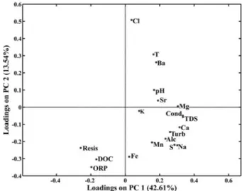
In the loadings plot (Figure 6), it can be observed that Fe and DOC are near indicating some similarity between them, although they are presented in different quadrants. The argument for the scores plot is valid here, since all variance in the data set is not represented. The
Figure 4. Concentration of sulfate in selected water samples from the
Quadrilátero Ferrífero.
Figure 5. Scores plot on PC1 and PC2 in the study of dissolved organic
matter and metal ions in waters from the eastern Quadrilátero Ferrífero, Brazil.
Figure 6. Loadings plot on PC1 and PC2 in the study of dissolved
relationships among DOC, Fe, ORP and Resis in Kohonen map (Figure 3) are also demonstrated in the loadings plot (Figure 6).
In general, the main tendencies (greater similarities or differences among samples or variables, and the influences of variables in samples) of the data set were shown by both the Kohonen neural network and the PCA methods, although the PCA was not able to present all data variance while Kohonen neural network expressed it very efficiently in a two-dimensional space.
Conclusions
The multivariate exploratory data analysis by the application of Kohonen neural network was effective in this study, especially considering an easy and friendly data interpretation, with complex nonlinear relationships. Furthermore, this technique allowed a separation of all samples into groups with similar characteristics while reducing a high dimensional space to a two-dimensional space. It was one of the main advantages of this technique when compared with PCA, which was applied to the same data set. In the latter method, it was necessary to work in a multidimensional space (11 PC) making the analysis of the results difficult. Nevertheless, both methods showed similar relationships of the data set.
A positive relationship between DOC and Fe was noted in the Kohonen neural network. This observation possibly indicates a complexation between both variables as described in the literature. A certain influence of seasonality on the distribution of samples could be noticed considering that some groups in the Kohonen map were formed as a result of their sampling date (rainy or dry period). In addition, some samples that were collected at the same point in different seasons stayed in different groups due to the effects of leaching or dilution. Some relationships among some elements in the Kohonen neural network indicated a contribution from the lithology of the studied area as it can be found by the elements Ca, Mg, Mn and Sr in the maps of the distribution of variables. Chloride may be partly also from biogenic origin since the rocks in the region studied do not have Cl in their structure.
Further studies will be necessary to measure and characterise the dissolved organic matter in the area and to fully understand its role on the cycle of elements in the QF, especially considering the impacts of mining. However, in this study it was possible to perform a screening of the evaluated area, particularly considering the concentrations of DOC and of some metal ions. In addition, the use of the Kohonen neural network for the first time with chemical data of this studied area showed that it certainly is a
promising technique that may help to analyse a variety of environmental results with complex interdependencies in an easy way.
Supplementary Information
Supplementary information (Figure S1) is available free of charge at http://jbcs.sbq.org.br as PDF file.
Acknowledgements
The authors of this paper gratefully acknowledge CAPES, CNPq, FAPEMIG, Fundação Gorceix and UFOP for financial support for this research.
References
1. Deschamps, E.; Ciminelli, V.; Lange, F.; Matschullat, J.; Raue, B.; Schmidt, H.; J. Soils Sediments2002, 2, 216. 2. Mikutta, C.; Kretzschmar, R.; Environ. Sci. Technol.2011, 45,
9550.
3. Borba, R. P.; Figueiredo, B. R.; Matschullat, J.; Environ. Geol. 2003, 44, 39.
4. Varcjao, E. V. V.; Bellato, C. R.; Fontes, M. P. F.; Mello, J. W. V.;
Environ. Monit. Assess.2011, 172, 631.
5. Pereira, A.; van Hattum, B.; Brouwer, A.; van Bodegom, P.; Rezende, C.; Salomons, W.; J. Soils Sediments2008, 8, 239. 6. McDonald, S.; Bishop, A. G.; Prenzler, P. D.; Robards, K.; Anal.
Chim. Acta2004, 527, 105.
7. Wood, C. M.; Al-Reasi, H. A.; Smith, D. S.; Aquat. Toxicol. 2011, 105, 3.
8. Ravichandran, M.; Chemosphere2004, 55, 319.
9. Castro, G. R.; Padilha, C. C. F.; Rocha, J. C.; Valente, J. P. S.; Florentino, A. O.; Padilha, P. M.; Ecletica Quim. 2005,
30, 45.
10. de Oliveira, L. C.; Sargentini Jr, E.; Rosa, A. H.; Rocha, J. C.; Simões, M. L.; Martin-Neto, L.; Silva, W. T. L.; Serudo, R. L.;
J. Braz. Chem. Soc.2007, 18, 860.
11. Rogers, J.; Object-oriented Neural Networks in C++; Academic Press: San Diego, CA, USA, 1997.
12. Garcia, J. S.; da Silva, G. A.; Arruda, M. A. Z.; Poppi, R. J.;
X-Ray Spectrom.2007, 36, 122.
13. Çinar, O.; Merdun, H.; Ecol. Res.2009, 24, 163.
14. Gamble, A.; Babbar-Sebens, M.; Environ. Monit. Assess.2012,
184, 845.
15. Çinar, O.; Process Biochem.2005, 40, 2980.
16. Lee, W. S.; Kwon, Y. S.; Yoo, J. C.; Song, M. Y.; Chon, T. S.;
Ecol. Modell. 2006, 193, 602. 17. Chon, T. S.; Ecol. Info.2011, 6, 50.
18. Kottek, M.; Grieser, J.; Beck, C.; Rudolf, B.; Rubel, F.;
19. de Sá Júnior, A.; de Carvalho, L. G.; da Silva, F. F.; Alves, M. de C.; Theor. Appl. Climatol.2012, 108, 1.
20. APHA; AWWA; WEF; Standard methods for the examination of water and wastewater, 21st ed.; American Public Health Association, American Water Works Association and Water Environment Federation: Washington, D.C., 2005.
21. Grasshoff, K.; Kremling, K.; Ehrhardt, M.; Methods of Seawater Analysis, 3rd ed.; Wiley-VCH: New York, 1999.
22. Alhoniemi, E.; Himberg, J.; Parhankangas, J.; Vesanto, J.; Laboratory of Computer and Information Science, Finland, 2000. Available at http://www.cis.hut.fi/projects/ somtoolbox/, accessed in November, 2013.
23. Dorr, J. V. N.; Physiographic, Stratigraphic and Structural Development of the Quadrilátero Ferrífero, Minas Gerais,
Brazil, U.S.G.S. Professional Paper 641-A: Washington, 1969. 24. Alkmim, F. F.; Marshak, S.; Precambrian Res.1998, 90, 29. 25. Kohonen, T.; Self-Organizing Maps, 3rd ed.; Springer: Berlin/
Heidelberg/New York, 2001.
26. Environmental Control Agency of São Paulo State (CETESB);
Significado ambiental e sanitário das variáveis de qualidade
das águas e dos sedimentos e metodologias analíticas e de
amostragem; CETESB: São Paulo, SP, Brasil, 2009.
27. Laglera, L. M.; Battaglia, G.; van den Berg, C. M. G.; Mar. Chem.2011, 127, 134.
28. Laglera, L. M.; Battaglia, G.; van den Berg, C. M. G.; Anal. Chim. Acta2007, 599, 58.
29. Steinberg, C.; Ecology of Humic Substances in Freshwaters, Springer-Verlag: Berlin, 2003.
30. Stevenson, F. J.; Humus Chemistry: Genesis, Composition and Reactions, 2nd ed.; John Wiley & Sons: New York, 1994.
Submitted: August 12, 2013