Non-singular spherical harmonic expressions of geomagnetic vector and gradient tensor fields in the local north-oriented reference frame

(1)

GMDD

7, 8477–8503, 2014

Non-singular spherical harmonic

expressions of geomagnetic fields

J. Du et al.

Title Page

Abstract Introduction

Conclusions References

Tables Figures

◭ ◮

Back Close

Full Screen / Esc

Printer-friendly Version Interactive Discussion

Discussion

P

a

per

|

Discussion

P

a

per

|

Discussion

P

a

per

|

Discussion

P

a

per

|

Geosci. Model Dev. Discuss., 7, 8477–8503, 2014 www.geosci-model-dev-discuss.net/7/8477/2014/ doi:10.5194/gmdd-7-8477-2014

This discussion paper is/has been under review for the journal Geoscientific Model Development (GMD). Please refer to the corresponding final paper in GMD if available.

Non-singular spherical harmonic

expressions of geomagnetic vector and

gradient tensor fields in the local

north-oriented reference frame

J. Du1,2,3,4, C. Chen1,3, V. Lesur2, and L. Wang1,3,4

1

Institute of Geophysics & Geomatics, China University of Geosciences, Wuhan 430074, China

2

Helmholtz Centre Potsdam, GFZ German Research Centre for Geosciences, 14473 Telegrafenberg, Germany

3

Hubei Subsurface Multi-scale Imaging Lab (SMIL), China University of Geosciences, Wuhan 430074, China

4

State Key Laboratory of Geodesy and Earth’s Dynamics, Chinese Academy of Sciences, Wuhan 430077, China

Received: 27 October 2014 – Accepted: 4 November 2014 – Published: 5 December 2014

Correspondence to: J. Du ([email protected])

(2)

GMDD

7, 8477–8503, 2014

J. Du et al.

Title Page

Tables Figures

◭ ◮

Back Close

Full Screen / Esc

Discussion

P

a

per

|

Discussion

P

a

per

|

Discussion

P

a

per

|

Discussion

P

a

per

|

Abstract

General expressions of magnetic vector (MV) and magnetic gradient tensor (MGT) in terms of the first- and second-order derivatives of spherical harmonics at different degrees and orders, are relatively complicated and singular at the poles. In this paper, we derived alternative non-singular expressions for the MV, the MGT and also the 5

higher-order partial derivatives of the magnetic field in local north-oriented reference frame. Using our newly derived formulae, the magnetic potential, vector and gradient tensor fields at an altitude of 300 km are calculated based on a global lithospheric magnetic field model GRIMM_L120 (version 0.0) and the main magnetic field model of IGRF11. The corresponding results at the poles are discussed and the validity of the 10

derived formulas is verified using the Laplace equation of the potential field.

1 Introduction

Compared to the magnetic vector and scalar measurements, magnetic gradients lead to more robust models of the lithospheric magnetic field. The ongoing ESA’sSwarm

mission, will provide measurements not only of the vector and scalar data but also 15

an estimate of their east–west gradients (e.g. Olsen et al., 2004; Friis-Christensen et al., 2006). Kotsiaros and Olsen (2012, 2014) proposed to recover the lithospheric magnetic field through Magnetic Space Gradiometry in the same way that has been done for modeling the gravitational potential field from the GOCE satellite gravity gradi-ent tensor measuremgradi-ents. Purucker et al. (2005, 2007) also reported efforts to model 20

the lithospheric magnetic field using magnetic gradient information from the Ørsted, CHAMP, SAC-C and ST-5 constellation. Their results showed that by using gradients data, the modelled lithospheric magnetic anomaly field has enhanced shorter wave-length content and has a much higher quality compared to models built from vector field data. This is because the gradients data can remove the highly time-dependant 25

(3)

GMDD

7, 8477–8503, 2014

J. Du et al.

Title Page

Tables Figures

◭ ◮

Back Close

Full Screen / Esc

Discussion

P

a

per

|

Discussion

P

a

per

|

Discussion

P

a

per

|

Discussion

P

a

per

|

contributions of the magnetosphere and ionosphere that are correlated between two side-by-side satellites.

The order-2 magnetic gradient tensor consists of spatial derivatives highlighting cer-tain structures of the magnetic field (e.g. Schmidt and Clark, 2000, 2006). It can be used to detect the hidden and small-scale magnetized sources (e.g. Pedersen and 5

Rasmussen, 1990; Harrison and Southam, 1991) and to investigate the orientation of the lineated magnetic anomalies (e.g. Blakely and Simpson, 1986). Quantitative mag-netic interpretation methods such as the analytic signal, edge detection, spatial deriva-tives, Euler deconvolution, and transforms, all set in Cartesian coordinate system (e.g. Blakely, 1995; Purucker and Whaler, 2007; Taylor et al., 2014) also require calculating 10

the higher-order derivatives of the magnetic anomaly field and need to be extended to regional and global scales to handle the curvature of the Earth and other planets. Ravat et al. (2002) and Ravat (2011) utilized the analytic signal method and the to-tal gradient to interpret the satellite-altitude magnetic anomaly data. Therefore, both the magnetic field modelling and also the geological interpretations require the calcu-15

lation for the partial derivatives of the magnetic field in form of spherical harmonics, possibly at the poles for specific systems of coordinates. Spherical harmonic analysis (SHA), established originally by Gauss (1839), is generally used to model the global magnetic lithospheric field of the Earth and other terrestrial planets (e.g. Maus et al., 2008; Langlais et al., 2009; Thébault et al., 2010; Lesur et al., 2013; Sabaka et al., 20

2013; Olsen et al., 2014). Series of spherical harmonic functions themselves made of Schmidt semi-normalized associated Legendre functions (SSALFs) (e.g. Blakely, 1995; Langel and Hinze, 1998), are fitted by least-squares to magnetic measurements, giving the spherical harmonic coefficients i.e. the Gaussian coefficients defining the model. Kotsiaros and Olsen (2012, 2014) presented the MV and the MGT using a spherical 25

(4)

GMDD

7, 8477–8503, 2014

J. Du et al.

Title Page

Tables Figures

◭ ◮

Back Close

Full Screen / Esc

Discussion

P

a

per

|

Discussion

P

a

per

|

Discussion

P

a

per

|

Discussion

P

a

per

|

airborne or shipborne magnetic data are utilized (e.g. Golynsky et al., 2013; Maus, 2010).

In this paper, following Petrovskaya and Vershkov (2006) and Eshagh (2008, 2009) for the gravitational gradient tensor in the local-north-oriented reference frame (LNORF), the non-singular expressions in terms of spherical harmonics for the MV, the 5

MGT and the higher-order derivatives of the magnetic anomaly field in the LNORF are presented. In the next section, the traditional expressions of the MV and the MGT are first stated, then some necessary propositions are proved and at last new non-singular expressions are derived. In Sect. 3, the new formulae are tested using the global litho-spheric magnetic field model GRIMM_L120 (version 0.0) (Lesur et al., 2013) and the 10

main magnetic field model of IGRF11 (Finlay et al., 2010). Finally, further applications are discussed and some conclusions are also drawn.

2 Methodology

In this section, the traditional expressions of MV and MGT are presented, and their numerical problems are stated. Then based on the mathematical derivations, new ex-15

pressions are given.

2.1 Traditional expressions

The scalar potential V of the Earth’s magnetic field in a source-free region can be expanded in the truncated series of spherical harmonics at the point P(r,θ,ϕ) (e.g. Backus et al., 1996):

20

V(r,θ,ϕ)=a

L

X

l=1

l

X

m=0

_a

r

l+1

gm_l cosmϕ+hm_l sinmϕ eP_lm(cosθ), (1)

wherea=6371.2 km is the radius of the Earth’s magnetic reference sphere; r,θand

(5)

GMDD

7, 8477–8503, 2014

J. Du et al.

Title Page

Tables Figures

◭ ◮

Back Close

Full Screen / Esc

Discussion

P

a

per

|

Discussion

P

a

per

|

Discussion

P

a

per

|

Discussion

P

a

per

|

simplification) is the SSALF of degree l and order m; L is the maximum spherical harmonic degree; g_lm and hm_l are the geomagnetic harmonic coefficients describing internal sources of the Earth.

If considered in the LNORFxP,yP,zP at the pointP(r,ϕ,θ), wherezP axis points

downward in geocentric radial direction, xP axis points to the north, and yP axis

to-5

wards the east (that is, a right-handed system). At the poles, we define that y_P axis points to the meridian of 90◦E. Therefore, the three components of the MV can be expressed as:

Bx(r,θ,ϕ)=−

1

r ∂

∂(₋θ)V(r,θ,ϕ)

=

L

X

l=1

l

X

m=0

_a

r

l+2

gm_l cosmϕ+hm_l sinmϕ

∂ ∂θPe

m l (cosθ)

, (2a) 10

B_y(r,θ,ϕ)=−_r 1 sinθ

∂

∂ϕV(r,θ,ϕ)

=

L

X

l=1

l

X

m=0

_a

r

l+2

m g_lmsinmϕ−hm_l cosmϕ

1 sinθPe

m l (cosθ)

, (2b)

Bz(r,θ,ϕ)=−

∂

∂(−r)V(r,θ,ϕ)

=−

L

X

l=1

l

X

m=0

(l+1)a

r

l+2

gm_l cosmϕ+hm_l sinmϕ eP_lm(cosθ). (2c)

The MGT can be written as (e.g. Kotsiaros and Olsen, 2012) 15

∇B₌

 

B_xx B_xy B_xz Byx Byy Byz

B_zx B_zy B_zz



₌

 

∂B_x/∂x ∂B_x/∂y ∂B_x/∂z ∂By/∂x ∂By/∂y ∂By/∂z

∂B_z/∂x ∂B_z/∂y ∂B_z/∂z



(6)

GMDD

7, 8477–8503, 2014

J. Du et al.

Title Page Abstract Introduction Conclusions References Tables Figures ◭ ◮ ◭ ◮ Back Close

Full Screen / Esc

Printer-friendly Version Interactive Discussion Discussion P a per | Discussion P a per | Discussion P a per | Discussion P a per |

where nine elements are expressed respectively as:

B_xx=1_a

L

X

l=1

l

X

m=0

_a

r

l+3

×

"

− ∂ 2

∂θ2Pe

m

l (cosθ)+(l+1)Pe m l (cosθ)

#

, (4a)

B_xy =B_yx=1

a

L

X

l=1

l

X

m=0

_a

r

l+3

m gm_l sinmϕ₋hm_l cosmϕ

×

− 1 sinθ

∂ ∂θPe

m

l (cosθ)+

cosθ

sin2θ

e

P_lm(cosθ)

, (4b)

5

Bxz =Bzx=

1

a

L

X

l=1

l

X

m=0

_a

r

l+3

(l+2) g_lmcosmϕ+hm_l sinmϕ

_∂

∂θPe

m l (cosθ)

, (4c)

Byy =

1

a

L

X

l=1

l

X

m=0

_a

r

l+3

×

"

(l+1)Pe_lm(cosθ)+ m

2

sin2θPe

m

l (cosθ)−

cosθ

sinθ ∂ ∂θPe

m l (cosθ)

#

, (4d)

Byz=Bzy=

1

a

L

X

l=1

l

X

m=0

_a

r

l+3

(l+2)m g_lmsinmϕ−hm_l cosmϕ

1 sinθPe

m l (cosθ)

,

(4e)

B_zz=−1_a

L

X

l=1

l

X

m=0

_a

r

l+3

(l+1)(l+2) g_lmcosmϕ+hm_l sinmϕ eP_lm(cosθ). (4f) 10

The expressions for B_z and B_zz can be calculated stably even for very high SH de-grees and orders by using the Holmes and Featherstone (2002a) scheme. However,

(7)

GMDD

7, 8477–8503, 2014

J. Du et al.

Title Page

Tables Figures

◭ ◮

Back Close

Full Screen / Esc

Discussion

P

a

per

|

Discussion

P

a

per

|

Discussion

P

a

per

|

Discussion

P

a

per

|

there exist the singular terms of 1/sinθand 1/sin2θin Eqs. (2b), (4b), (4d) and (4e) when the computing point approaches to the poles. Besides, some expressions con-tain the terms of first- and second-order derivatives of SSALFs, such as Eqs. (2a) and (4a)–(4d). Nevertheless, the second-order derivative for very high degree and or-ders of SSALFs can be recursively calculated by the Clenshaw or Horner algorithms 5

(Holmes and Featherstone, 2002b). These algorithms are relatively complicated and thus we want to use alternative expressions to avoid the singular terms and the partial derivatives of SSALFs.

2.2 Mathematical derivations

To deal with the singular terms and first- and second-order derivatives of the SSALFs, 10

some useful mathematical derivations are introduced and proved in the following.

1 – Derivation of∂Pe_lm/∂θ

Based on the Eq. (Z.1.44) in Ilk (1983)

∂P_lm/∂θ=0.5(l+m)(l−m+1)P_lm−1−P_lm+1, (5) and the relation between the ALFs and the SSALFs as

15

e

P_lm=

q

Cm(l−m)!/(l+m)!P_lm, (6)

thus the first-order derivative of the SSALFs can be deduced as:

∂Pe_lm/∂θ=a_l,mPelm−1+bl,mPelm+1, (7a)

a_l,m=0.5

p

l+mpl₋m+1

q

C_m/C_m₋1, (7b)

b_l,m=−0.5

p

l+m+1pl₋m

q

C_m/C_m₊1, (7c)

(8)

GMDD

7, 8477–8503, 2014

J. Du et al.

Title Page

Tables Figures

◭ ◮

Back Close

Full Screen / Esc

Discussion

P

a

per

|

Discussion

P

a

per

|

Discussion

P

a

per

|

Discussion

P

a

per

|

whereCm=2−δm,0=

(

1, m=0

2, m6=0 andδis the Kronecker’s delta function.

2 – Derivation of∂2_P_em l /∂θ

2

According to the Eq. (23) in Eshagh (2008) as

∂2P_lm/∂θ2=0.25(l+m)(l₋m+1)(l+m₋1)(l₋m+2)P_lm−2

−0.25(l+m)(l₋m+1)+(l₋m)(l+m+1)P_lm+0.25P_lm+2, (8) 5

the second-order derivative of the SSALFs can be written as:

∂2Pe_lm/∂θ2=cl,mPe_lm−2+dl,mPe_lm+el,mPe_lm+2, (9a)

cl,m=0.25

p

l+mpl+m−1pl−m+2pl−m+1

q

Cm/Cm₋2, (9b) dl,m=−0.25

(l+m)(l−m+1)+(l−m)(l+m+1), (9c)

el,m=0.25

p

l+m+2pl+m+1pl−mpl−m−1

q

Cm/Cm+2. (9d) 10

3 – Derivation ofPe_lm/sinθ

Using the Eq. (Z.1.42) in Ilk (1983)

P_lm/sinθ=0.5(l+m)(l+m−1)P_lm₋₁−1+P_lm₋₁+1/m, m≥1, (10) and the Eq. (6), we can obtain that

e

P_lm/sinθ=f_l,mPelm₋1−1+gl,mPe

m+1

l₋1 ,m≥1, (11a) 15

fl,m=0.5

p

l+mpl+m−1

q

Cm/Cm₋1/m, m≥1, (11b) gl,m=0.5

p

l−mpl−m−1

q

Cm/Cm+1/m, m≥1. (11c)

(9)

GMDD

7, 8477–8503, 2014

J. Du et al.

Title Page

Tables Figures

◭ ◮

Back Close

Full Screen / Esc

Discussion

P

a

per

|

Discussion

P

a

per

|

Discussion

P

a

per

|

Discussion

P

a

per

|

4 – Derivation ofPe_lm/sin2θ

Employing the Eq. (31) in Eshagh (2008) as

P_lm/sin2θ={(l+m)(l+m−1)(l−m+1)(l−m+2)/(m−1)P_lm−2

+(l+m)(l+m−1)/(m−1)₊(l−m)(l−m−1)/(m+1)P_lm

+1/(m+1)P_lm+2}/(4m), m≥2, (12) 5

and the Eq. (6), we have

e

P_lm/sin2θ=h_l,mPem−

2

l +kl,mPelm+nl,mPelm+2, m≥2, (13a)

h_l,m=0.25

p

l+mpl+m−1pl−m+1pl−m+2

q

C_m/C_m₋2/

m(m−1), m≥2, (13b)

k_l,m=0.25

(l+m)(l+m₋1)/(m₋1)+(l₋m)(l₋m₋1)/(m+1)/m, m_≥2, (13c)

n_l,m=0.25

p

l−mpl−m−1pl+m+2pl+m+1

q

C_m/C_m₊2/

m(m+1), m≥1. (13d) 10

5 – Derivation of∂Pe_lm/(sinθ∂θ)

Using the Eq. (36) in Eshagh (2008) as

∂P_lm/(sinθ∂θ)=0.25_{(l+m)(l+m−1)(l+m−2)(l−m+1)/(m−1)P_lm₋₁−2

+(l+m)(l₋m+1)/(m₋1)₋(l+m+1)(l+m)/(m+1)P_lm −1

−1/(m+1)P_lm₋₁+2_}, m≥2, (14)

(10)

GMDD

7, 8477–8503, 2014

J. Du et al.

Title Page

Tables Figures

◭ ◮

Back Close

Full Screen / Esc

Discussion

P

a

per

|

Discussion

P

a

per

|

Discussion

P

a

per

|

Discussion

P

a

per

|

and the Eq. (6), we can derive

∂Pe_lm/(sinθ∂θ)=o_l,mPelm₋1−2+ql,mPe

m

l₋1+xl,mPe

m+2

l₋1 , m≥2, (15a) o_l,m=0.25

p

l+mpl+m−1pl+m−2pl−m+1

q

C_m/C_m₋2/(m−1), m≥2,

(15b)

q_l,m=0.25

p

l₋mpl+m(l₋m+1)/(m₋1)₋(l+m+1)/(m+1), m_≥2, (15c)

xl,m=−0.25

p

l+m+1pl−mpl−m−1pl−m−2

q

Cm/Cm+2/(m+1). (15d) 5

6 – Derivation of∂Pe_lm/(sinθ∂θ)−Pe_lmcosθ/sin2θ

According to Petrovskaya and Vershkov (2006) and Eshagh (2009), we can write

∂P_lm/(sinθ∂θ)₋P_lmcosθ/sin2θ=

0.5(m₋1)(l+m)(l₋m+1)P_lm−1/sinθ₋(m+1)Pm+1

l /sinθ

/m, m_≥1, (16)

and using the Eq. (36) in Eshagh (2008), we can obtain 10

P_lm−1/sinθ=0.5(l−m+2)(l−m+3)P_lm₊₁−2+P_lm₊₁/(m−1), m≥2, (17a)

P_lm+1/sinθ=0.5(l−m)(l−m+1)P_lm₊₁+P_lm₊₁+2/(m+1). (17b) Substituting the Eq. (17) into the right hand side of the Eq. (16) and after simplification, we can derive

∂P_lm/(sinθ∂θ)₋P_lmcosθ/sin2θ=0.25(l+m)(l−m+1)(l−m+2)(l−m+3)P_lm₊−₁2

15

+2m(l₋m+1)P_lm₊₁₋Pm+2

l+1

/m, m_≥1. (18)

(11)

GMDD

7, 8477–8503, 2014

J. Du et al.

Title Page

Tables Figures

◭ ◮

Back Close

Full Screen / Esc

Discussion

P

a

per

|

Discussion

P

a

per

|

Discussion

P

a

per

|

Discussion

P

a

per

|

And combing the Eq. (6), we obtain that

∂Pe_lm/(sinθ∂θ)−Pe_lmcosθ/sin2θ=

0.25hpl+mpl−m+1pl−m+2pl−m+3

q

Cm/Cm₋2Pem− 2

l+1

+2mpl₋m+1pl+m+1Pe_lm₊₁

−pl+m+1pl+m+2pl+m+3pl−m

q

Cm/Cm+2Pe_lm₊1+2

i

/m, m≥1. (19) 5

7 – Derivation of(l+1)sin2θPem

l +m

2_P_em

l −sinθcosθ∂Pe_lm/∂θ

/sin2θ

Based on the Lemma 3 in Eshagh (2009) as

sinθcosθ∂P_lm/∂θ=mP_lm+(l+1)sin2θP_lm−sinθP_lm₊₁+1, (20) we can derive

(l+1)sin2θP_lm+m2_Pm

l −sinθcosθ∂P m l /∂θ

/sin2θ= 10

m(m−1)P_lm/sin2θ+P_lm₊₁+1/sinθ. (21) According to the Eq. (10), we can write

Pm+1

l+1 /sinθ=0.5

(l+m+2)(l+m+1)P_lm+Pm+2

l

/(m+1). (22)

Inserting the Eqs. (12) and (22) into the Eq. (21), and after some simplifications, we obtain that

15

(l+1)sin2θP_lm+m2P_lm₋sinθcosθ∂P_lm/∂θ/sin2θ= 0.25(l+m)(l+m−1)(l−m+1)(l−m+2)P_lm−2

+0.25(l+m)(l+m−1)+(l−m)(l−m−1)(m−1)/(m+1)

(12)

GMDD

7, 8477–8503, 2014

J. Du et al.

Title Page

Tables Figures

◭ ◮

Back Close

Full Screen / Esc

Discussion

P

a

per

|

Discussion

P

a

per

|

Discussion

P

a

per

|

Discussion

P

a

per

|

And combing with the Eq. (6), we can derive

(l+1)sin2θPe_lm+m2_P_em

l −sinθcosθ∂Pe m l /∂θ

/sin2θ=

0.25pl+mpl+m₋1pl₋m+1pl₋m+2

q

C_m/C_m₋2Pe_lm−2

+0.25(l+m)(l+m−1)+(l−m)(l−m−1)(m−1)/(m+1) +2(l+m+2)(l+m+1)/(m+1) eP_lm

5

+0.25pl+m+1pl+m+2pl₋mpl₋m₋1

q

C_m/C_m₊2Pe_lm+2. (24)

2.3 New expressions

Inserting the corresponding mathematical derivations in the last section into the Eqs. (2) and (4) and after some simplifications, the new expressions for the MV and the MGT can be written as:

10

B_x=

L

X

l=1

l

X

m=0

_a

r

l+2

gm_l cosmϕ+hm_l sinmϕax_l_,_mPe_lm−1+bx_l_,_mPem+1

l

, (25a)

B_y=

L

X

l=1

l

X

m=0

_a

r

l+2

g_lmsinmϕ₋hm_l cosmϕay_l_,_mPe_lm−1 −1 +b

y l,mPe

m+1

l₋1

, (25b)

B_z=

L

X

l=1

l

X

m=0

_a

r

l+2

gm_l cosmϕ+hm_l sinmϕaz_l_,_mPe_lm, (25c)

B_xx=1_a

L

X

l=1

l

X

m=0

_a

r

l+3

gm_l cosmϕ+hm_l sinmϕaxx_l_,_mPe_lm−2+bxx_l_,_mPe_lm+cxx_l_,_mPe_lm+2,

(26a) 15

(13)

GMDD

7, 8477–8503, 2014

J. Du et al.

Full Screen / Esc

B_xy=_a1

L

X

l=1

l

X

m=0

_a

r

l+3

g_lmsinmϕ₋hm_l cosmϕaxy_l_,_mPe_lm₊₁−2+bxy_l_,_mPe_lm₊₁+c_lxy_,_mPe_lm₊₁+2,

(26b)

B_xz=1_a

L

X

l=1

l

X

m=0

_a

r

l+3

gm_l cosmϕ+hm_l sinmϕaxz_l_,_mPe_lm−1+bxz_l_,_mPe_lm+1, (26c)

B_yy=1_a

L

X

l=1

l

X

m=0

_a

r

l+3

g_lmcosmϕ+hm_l sinmϕayy_l_,_mPe_lm−2+byy_l_,_mPe_lm+cyy_l_,_mPe_lm+2,

(26d)

Byz=

1

a

L

X

l=1

l

X

m=0

_a

r

l+3

gm_l sinmϕ−hm_l cosmϕayz_l_,_mPe_lm₋₁−1+byz_l_,_mPe_lm₋+₁1, (26e)

Bzz=

1

a

L

X

l=1

l

X

m=0

_a

r

l+3

gm_l cosmλ+hm_l sinmϕazz_l_,_mPe_lm. (26f) 5

Furthermore, some other higher-order partial derivatives and their transforms are usu-ally used to image geologic boundaries in magnetic prospecting (e.g. Hsu et al., 1996). Therefore, we also give the third-order partial derivatives of the spherical harmonics as following:

B_xxz=∂Bxx

∂z = ∂2Bx

∂x∂z= ∂2Bx

∂z∂x 10 = 1 a2 L X

l=1

l

X

m=0

_a

r

l+4

gm_l cosmϕ+hm_l sinmϕaxxz_l_,_mPe_lm−2+bxxz_l_,_mPe_lm+cxxz_l_,_mPe_lm+2,

(27a)

B_xyz=∂Bxy

∂z = ∂Byx

∂z = ∂2Bx

∂y∂z= ∂2Bx

∂z∂y = ∂2By

∂x∂z = ∂2By

(14)

GMDD

7, 8477–8503, 2014

J. Du et al.

Full Screen / Esc

Printer-friendly Version Interactive Discussion Discussion P a per | Discussion P a per | Discussion P a per | Discussion P a per | = 1 a2 L X

l=1

l

X

m=0

_a

r

l+4

gm_l sinmϕ₋hm_l cosmϕaxyz_l_,_mPe_lm₊−₁2+bxyz_l_,_mPe_lm₊₁+c_lxyz_,_mPe_lm₊₁+2,

(27b)

B_xzz=∂Bxz

∂z = ∂Bzx

∂z = ∂2Bx

∂z2 = ∂2Bz

∂x∂z = ∂2Bz

∂z∂x

= 1

a2

L

X

l=1

l

X

m=0

_a

r

l+4

gm_l cosmϕ+hm_l sinmϕaxzz_l_,_mPe_lm−1+bxzz_l_,_mPe_lm+1, (27c)

B_yyz=∂Byy

∂z = ∂2By

∂y∂z = ∂2By

∂z∂y

= 1

a2

L

X

l=1

l

X

m=0

_a

r

l+4

gm_l cosmϕ+hm_l sinmϕayyz_l_,_mPe_lm−2+byyz_l_,_mPe_lm+cyyz_l_,_mPe_lm+2,

(27d) 5

B_yzz=∂Byz

∂z = ∂Bzy

∂z = ∂2By

∂z2 = ∂2Bz

∂y∂z= ∂2Bz

∂z∂y

= 1

a2

L

X

l=1

l

X

m=0

_a

r

l+4

gm_l sinmλ−hm_l cosmλayzz_l_,_mPe_lm₋₁−1+byzz_l_,_mPe_lm₋+₁1, (27e)

B_zzz=∂

2 Bz ∂z2 = 1 a2 L X

l=1

l

X

m=0

_a

r

l+4

gm_l cosmϕ+hm_l sinmϕazzz_l_,_mPe_lm, (27f)

where the corresponding coefficients of the SSALFs are presented in Appendix A and 10

can be computed once for all points. In this way, we avoid computing recursively the

(15)

GMDD

7, 8477–8503, 2014

J. Du et al.

Title Page

Tables Figures

◭ ◮

Back Close

Full Screen / Esc

Discussion

P

a

per

|

Discussion

P

a

per

|

Discussion

P

a

per

|

Discussion

P

a

per

|

SSALFs, their first- and second-order derivatives respectively with the traditional for-mulae. These new relations do not suffer from the singular terms and don’t contain the derivatives. The cost is only to calculate two additional degrees and orders for the SSALFs at most. In this study, we use the conventional form of SSALF that ifm < 0, thenPe_lm=(−1)|m|Pe_l|m| and ifm > l, thenPe_lm=0.

5

3 Numerical investigation

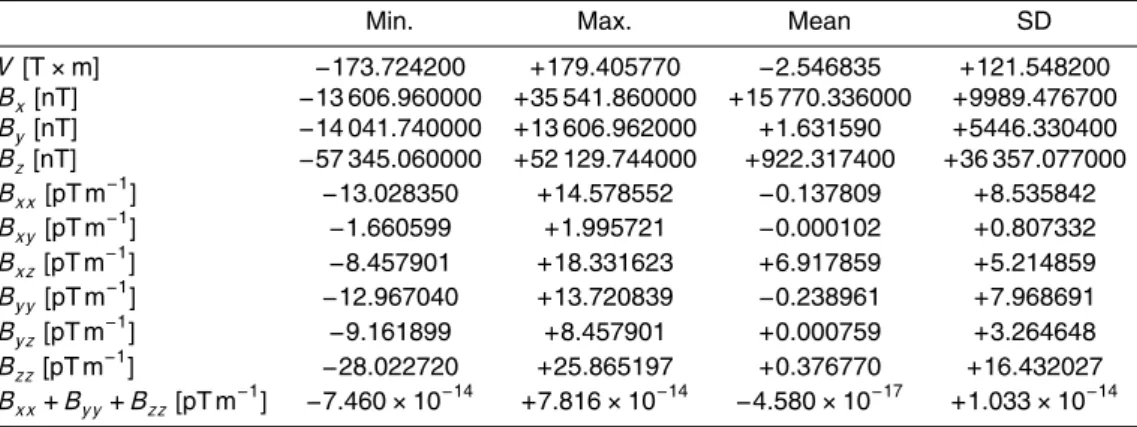
We test the derived expressions and the numerical implementation in C/C+ +, by cal-culating the magnetic potential, vector and its gradients on a grid with 0.125◦×0.125◦ cell size at the altitude of 300 km relative to the Earth’s magnetic reference sphere using the magnetic field models defined by: (i) the lithospheric magnetic field model 10

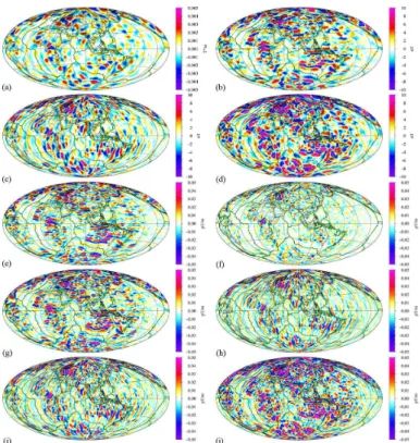
GRIMM_L120 (version 0.0) (Lesur et al., 2013); (ii) the main magnetic field model IGRF11 (Finlay et al., 2010) at the epoch of 2005.0.0. The global magnetic po-tential V, the MV and the MGT mapped by the lithospheric field and the main field are shown in Figs. 1 and 2, respectively. The corresponding statistics are pre-sented in Tables 1 and 2. A simple test is that the MGT meets the Laplace’s equa-15

tion of the potential field, that is, the trace of the MGT should be equal to zero. Our numerical results show that the amplitude of Bxx+Byy+Bzz is in the range of

[₋8.0_×10−14pT m−1/+8.0_×10−14pT m−1] (1 pT m−1=10−3nT m−1=1 nT km−1). The relative error is almost equal the machine accuracy. Therefore, this feature proves the validity of our derived formulae. In addition, as shown in Fig. 1, it is obvious that the 20

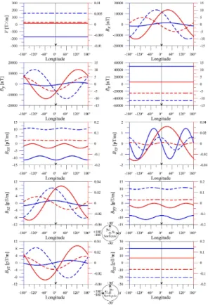
MGT enhances the lineation and contacts. It also reveals some small-scale anomalies, which is very helpful for the further geological interpretation. Figure 2 illustrates that the gradients of the main field are very smooth but the amplitudes are still very high. Furthermore, the computed magnetic fields are smooth near the poles and don’t have the singularities at the poles as shown in Fig. 3. The magnetic potentialV,Bz andBzz

25

(16)

How-GMDD

7, 8477–8503, 2014

J. Du et al.

Title Page

Tables Figures

◭ ◮

Back Close

Full Screen / Esc

Discussion

P

a

per

|

Discussion

P

a

per

|

Discussion

P

a

per

|

Discussion

P

a

per

|

ever, while changing with the direction of thexP andyP axes at the poles, theBx,By,

Bxz,Byzcomponents have a period of 360◦and theBxx,Bxy andByy components have

a period of 180◦. Therefore, at the poles we specially define that thex_P axis points to the meridian of 180◦E (or 180◦W) at north pole and 0◦E at south pole and theyP axis

points to the meridian of 90◦E, that is, the LNORF moving from Greenwich meridian to 5

the poles.

4 Discussion and conclusions

We develop in this paper the new expressions for the MV, the MGT and the third-order partial derivatives of the magnetic field in terms of spherical harmonics. The traditional expressions have complicated forms involving first- and second-order derivatives of the 10

SSALFs and are singular when approaching to the poles. Our newly derived formulae don’t contain the first- and second-order derivatives of the SSALFs and remove the singularities at the poles.

However, our formulae are derived in the spherical local north-oriented reference frame with specific definition at the poles. For an application to the magnetic data of 15

a satellite gradiometry mission, it is necessary to describe the MV and the MGT in the local orbital reference frame, where the new MV and MGT are the linear functions of the MV and the new MGT in the LNORF with coefficients related to the satellite track azimuth (e.g. Petrovskaya and Vershkov, 2006). The other main purpose of this paper is in the future to contribute to the signal processing and the geological interpretation 20

of lithospheric magnetic field model, especially in polar areas.

(17)

GMDD

7, 8477–8503, 2014

J. Du et al.

Full Screen / Esc

Appendix A: Additional formulae

Numerical constants in the Eqs. (25)–(27) are expressed in following:

  

ax_l_,_m=0.5√l+m√l−m+1

q

Cm/Cm−1 bx_l_,_m=−0.5√l+m+1√l₋m

q

C_m/C_m₊1,

(A1)

  

ay_l_,_m=0.5√l+m√l+m₋1

q

C_m/C_m₋1 by_l_,_m=0.5√l₋m√l₋m₋1

q

C_m/C_m₊1,

(A2)

az_l_,_m=−(l+1), (A3)

5       

axx_l_,_m=−0.25√l+m√l+m−1√l−m+2√l−m+1

q

Cm/Cm₋2 bxx_l_,_m=0.25(l+m)(l−m+1)+(l−m)(l+m+1)+(l+1)

cxx_l_,_m=−0.25√l+m+2√l+m+1√l−m√l−m−1

q

Cm/Cm+2,

(A4)       

axy_l_,_m=−0.25√l+m√l−m+1√l−m+2√l−m+3

q

C_m/C_m₋2 bxy_l_,_m=−0.5m√l−m+1√l+m+1

cxy_l_,_m=0.25√l+m+1√l+m+2√l+m+3√l₋m

q

C_m/C_m₊2,

(A5)

  

axz_l_,_m=0.5(l+2)√l+m√l₋m+1

q

C_m/C_m₋1=(l+2)axl,m

bxz_l_,_m=−0.5(l+2)√l+m+1√l−m

q

C_m/C_m₊1=(l+2)b

x l,m,

(A6)             

ayy_l_,_m=0.25√l+m√l+m−1√l−m+1√l−m+2

q

C_m/C_m₋2 byy_l_,_m=0.25(l+m)(l+m−1)+(l−m)(l−m−1)(m−1)/(m+1)

+2(l+m+2)(l+m+1)/(m+1)

cyy_l_,_m=0.25√l+m+1√l+m+2√l−m√l−m−1

q

Cm/Cm+2,

(18)

GMDD

7, 8477–8503, 2014

J. Du et al.

Full Screen / Esc

Printer-friendly Version Interactive Discussion Discussion P a per | Discussion P a per | Discussion P a per | Discussion P a per |   

ayz_l_,_m=0.5(l+2)√l+m√l+m−1

q

C_m/C_m₋1=(l+2)a

y l,m

byz_l_,_m=0.5(l+2)√l−m√l−m−1

q

Cm/Cm+1=(l+2)b

y l,m,

(A8)

azz_l_,_m=−(l+1)(l+2)=(l+2)az_l_,_m, (A9)

    

axxz_l_,_m =(l+3)axx_l_,_m bxxz_l_,_m =(l+3)bxx_l_,_m cxxz_l_,_m =(l+3)cxx_l_,_m,

(A10)     

axyz_l_,_m =(l+3)axy_l_,_m bxyz_l_,_m =(l+3)bxy_l_,_m cxyz_l_,_m =(l+3)cxy_l_,_m,

(A11)             

axzz_l_,_m =0.5(l+2)(l+3)√l+m√l₋m+1

q

C_m/C_m₋1

=(l+2)(l+3)ax_l_,_m=(l+3)axz_l_,_m bxzz_l_,_m =−0.5(l+2)(l+3)√l+m+1√l₋m

q

C_m/C_m₊₁

=(l+2)(l+3)bx_l_,_m=(l+3)bxz_l_,_m,

(A12) 5     

ayyz_l_,_m =(l+3)ayy_l_,_m byyz_l_,_m =(l+3)byy_l_,_m cyyz_l_,_m =(l+3)cyy_l_,_m,

(A13)             

ayzz_l_,_m =0.5(l+2)(l+3)√l+m√l+m−1

q

C_m/C_m₋1

=(l+2)(l+3)ay_l_,_m=(l+3)ayz_l_,_m byzz_l_,_m =0.5(l+2)(l+3)√l₋m√l₋m₋1

q

C_m/C_m₊1

=(l+2)(l+3)by_l_,_m=(l+3)byz_l_,_m,

(A14)

(19)

GMDD

7, 8477–8503, 2014

J. Du et al.

Title Page

Tables Figures

◭ ◮

Back Close

Full Screen / Esc

Discussion

P

a

per

|

Discussion

P

a

per

|

Discussion

P

a

per

|

Discussion

P

a

per

|

azzz_l_,_m =−(l+1)(l+2)(l+3)₌(l+3)azz_l_,_m=(l+2)(l+3)az_l_,_m. (A15) Code availability

Supplementary software implementation is performed by the programming language C/C+ +. The source code and input data presented in this paper can be obtained by contacting the corresponding author via email or download from the Supplement 5

related to the online version of this article.

The Supplement related to this article is available online at doi:10.5194/gmdd-7-8477-2014-supplement.

Acknowledgements. This study is supported by International Cooperation Projection in Science and Technology (No.: 2010DFA24580). Jinsong Du is sponsored by the China

Schol-10

arship Council (CSC). We would like to thank Mehdi Eshagh for his fruitful discussions. All projected figures are drawn using the Generic Mapping Tools (GMT) (Wessel and Smith, 1991).

The service charges for this open access publication have been covered by a Research Centre of the

15

Helmholtz Association.

References

Backus, G. E., Parker, R., and Constable, C.: Foundations of Geomagnetism, Cambridge Uni-versity Press, Cambridge, 1996.

Bird, P.: An updated digital model of plate boundaries, Geochem. Geophy. Geosy., 4, 1027,

20

doi:10.1029/2001GC000252, 2003.

Blakely, R. G.: Potential Theory in Gravity and Magnetic Applications, Cambridge University Press, New York, 1995.

Blakely, R. J. and Simpson, R. W.: Approximating edges of source bodies from magnetic or gravity anomalies, Geophysics, 51, 1494–1498, 1986.

25

(20)

GMDD

7, 8477–8503, 2014

J. Du et al.

Title Page

Tables Figures

◭ ◮

Back Close

Full Screen / Esc

Discussion

P

a

per

|

Discussion

P

a

per

|

Discussion

P

a

per

|

Discussion

P

a

per

|

Eshagh, M.: Alternative expressions for gravity gradients in local north-oriented frame and ten-sor spherical harmonics, Acta Geophys., 58, 215–243, 2009.

Finlay, C. C., Maus, S., Beggan, C. D., Bondar, T. N., Chambodut, A., Chernova, T. A., Chulliat, A., Golovkov, V. P., Hamilton, B., Hamoudi, M., Holme, R., Hulot, G., Kuang, W., Langlais, B., Lesur, V., Lowes, F. J., Lühr, H., Macmillan, S., Mandea, M., McLean, S.,

5

Manoj, C., Menvielle, M., Michaelis, I., Olsen, N., Rauberg, J., Rother, M., Sabaka, T. J., Tangborn, A., Tøffner-Clausen, L., Thébault, E., Thomson, A. W. P., Wardinski, I., Wei, Z., and Zvereva, T. I.: International geomagnetic reference field: the eleventh generation, Geo-phys. J. Int., 183, 1216–1230, 2010.

Friis-Christensen, E., Lühr, H., and Hulot, G.: Swarm: a constellation to study the Earth’s

mag-10

netic field, Earth Planets Space, 58, 351–358, 2006.

Gauss, C. F.: Allgemeine Theorie des Erdmagnetismus, in: Resultate aus den Beobachtungen des magnetischen Vereins im Jahre 1838, edited by: Gauss, C. F. and Weber, W., Weid-mannsche Buchhandlung, Leipzig, 1839, 1–57, 1838.

Golynsky, A., Bell, R., Blankenship, D., Damaske, D., Ferraccioli, F., Finn, C., Golynsky, D.,

15

Ivanov, S., Jokat, W., Masolov, V., Riedel, S., von Frese, R., Young, D., and ADMAP Working Group: Air and shipborne magnetic surveys of the Antarctic into the 21st century, Tectono-physics, 585, 3–12, 2013.

Harrison, C. and Southam, J.: Magnetic field gradients and their uses in the study of the Earth’s magnetic field, J. Geomagn. Geoelectr., 43, 485–599, 1991.

20

Holmes, S. A. and Featherstone, W. E.: A unified approach to the Clenshaw summation and the recursive computation of very high degree and order normalized associated Legendre functions, J. Geodesy, 76, 279–299, 2002a.

Holmes, S. A. and Featherstone, W. E.: SHORT NOTES: extending simplified high-degree syn-thesis methods to second latitudinal derivatives of geopotential, J. Geodesy, 76, 447–450,

25

2002b.

Hsu, S. K., Sibuet, J. C., and Shyu, C. T.: High-resolution detection of geologic boundaries from potential-field anomalies: an enhanced analytic signal technique, Geophysics, 61, 373–386, 1996.

Ilk, K. H.: Ein Beitrag zur Dynamik ausgedehnter Körper – Gravitationswechselwirkung, Reihe

30

C, Heft Nr. 288, Deutsche Geodätische Kommission, München, 1983.

Kotsiaros, S. and Olsen, N.: The geomagnetic field gradient tensor: properties and parametriza-tion in terms of spherical harmonics, Int. J. Geomath., 3, 297–314, 2012.

(21)

GMDD

7, 8477–8503, 2014

J. Du et al.

Title Page

Tables Figures

◭ ◮

Back Close

Full Screen / Esc

Discussion

P

a

per

|

Discussion

P

a

per

|

Discussion

P

a

per

|

Discussion

P

a

per

|

Kotsiaros, S. and Olsen, N.: End-to-End simulation study of a full magnetic gradiometry mission, Geophys. J. Int., 196, 100–110, 2014.

Langel, R. A. and Hinze, W. J.: The Magnetic Field of the Earth’s Lithosphere: the Satellite Perspective, Cambridge University Press, Cambridge, UK, 1998.

Langlais, B., Lesur, V., Purucker, M. E., Connerney, J. E. P., and Mandea, M.: Crustal magnetic

5

fields of terrestrial planets, Space Sci. Rev., 152, 223–249, 2010.

Lesur, V., Rother, M., Vervelidou, F., Hamoudi, M., and Thébault, E.: Post-processing scheme for modelling the lithospheric magnetic field, Solid Earth, 4, 105–118, doi:10.5194/se-4-105-2013, 2013.

Maus, S.: An ellipsoidal harmonic representation of Earth’s lithospheric magnetic field to degree

10

and order 720, Geochem. Geophy. Geosy., 11, Q06015, doi:10.1029/2010GC003026, 2010. Maus, S., Yin, F., Lühr, H., Manoj, C., Rother, M., Rauberg, J., Michaelis, I., Stolle, C., and

Müller, R. D.: Resolution of direction of oceanic magnetic lineations by the sixth-generation lithospheric magnetic field model from CHAMP satellite magnetic measurements, Geochem. Geophy. Geosy., 9, Q07021, doi:10.1029/2008GC001949, 2008.

15

Olsen, N. and the Swarm End-to-End Consortium: Swarm-End-to-End mission performance simulator study, ESA contract No. 17263/02/NL/CB, DSRI Report 1/2004, Danish Space Research Institute, Copenhagen, 2004.

Olsen, N., Lühr, H., Finlay, C. C., Sabaka, T. J., Michaelis, I., Rauberg, J., and Tøff ner-Clausen, L.: The CHAOS-4 geomagnetic field model, Geophys. J. Int., 197, 815–827, 2014.

20

Pedersen, L. B. and Rasmussen, T. M.: The gradient tensor of potential field anomalies: some implications on data collection and data processing of maps, Geophysics, 55, 1558–1566, 1990.

Petrovskaya, M. S. and Vershkov, A. N.: Non-singular expressions for the gravity gradients in the local north-oriented and orbital reference frames, J. Geodesy, 80, 117–127, 2006.

25

Purucker, M. E.: Lithospheric studies using gradients from close encounters of Ørsted, CHAMP and SAC-C, Earth Planets Space, 57, 1–7, 2005.

Purucker, M. and Whaler, K.: Crustal magnetism, in: Treatise on Geophysics, vol. 5, Geomag-netism, edited by: Kono, M., Elsevier, Amsterdam, 195–237, 2007.

Purucker, M., Sabaka, T., Le, G., Slavin, J. A., Strangeway, R. J., and Busby, C.: Magnetic

30

(22)

GMDD

7, 8477–8503, 2014

J. Du et al.

Title Page

Tables Figures

◭ ◮

Back Close

Full Screen / Esc

Discussion

P

a

per

|

Discussion

P

a

per

|

Discussion

P

a

per

|

Discussion

P

a

per

|

Ravat, D.: Interpretation of Mars southern highlands high amplitude magnetic field with total gradient and fractal source modeling: new insights into the magnetic mystery of Mars, Icarus, 214, 400–412, 2011.

Ravat, D., Wang, B., Wildermuth, E., and Taylor, P. T.: Gradients in the interpretation of satellite-altitude magnetic data: an example from central Africa, J. Geodyn., 33, 131–142, 2002.

5

Sabaka, T. J., Tøffner-Clausen, L., and Olsen, N.: Use of the comprehensive inversion method for swarm satellite data analysis, Earth Planets Space, 65, 1201–1222, 2013.

Schmidt, P. and Clark, D.: Advantages of measuring the magnetic gradient tensor, Preview, 85, 26–30, 2000.

Schmidt, P. and Clark, D.: The magnetic gradient tensor: its properties and uses in source

10

characterization, The Leading Edge, 25, 75–78, 2006.

Taylor, P. T., Kis, K. I., and Wittmann, G.: Satellite-altitude horizontal magnetic gradient anomalies used to define the Kursk magnetic anomaly, J. Appl. Geophys., 109, 133–139, doi:10.1016/j.jappgeo.2014.07.018, 2014.

Thébault, E., Purucker, M., Whaler, K. A., Langlais, B., and Sabaka, T. J.: The magnetic field of

15

Earth’s lithosphere, Space Sci. Rev., 155, 95–127, 2010.

Wessel, P. and Smith, W. H. F.: Free software helps map and display data, EOS Trans. AGU, 72, 441–446, 1991.

(23)

GMDD

7, 8477–8503, 2014

J. Du et al.

Title Page

Tables Figures

◭ ◮

Back Close

Full Screen / Esc

Discussion

P

a

per

|

Discussion

P

a

per

|

Discussion

P

a

per

|

Discussion

P

a

per

|

Table 1.Statistics of the global magnetic potential V, the MV and the MGT at the altitude of 300 km using the lithospheric magnetic field model GRIMM_L120 (version 0.0) (Lesur et al., 2013) for spherical harmonic degrees 16_∼90.

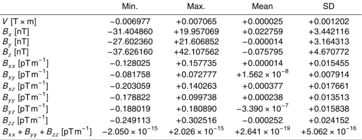
Min. Max. Mean SD

V [T×m] −0.006977 +0.007065 +0.000025 +0.001202

B_x[nT] ₋31.404860 +19.957069 +0.022759 +3.442116

B_y[nT] ₋27.602360 +21.606852 ₋0.000014 +3.164313

Bz[nT] −37.626160 +42.107562 −0.075795 +4.670772 Bxx[pT m−1] −0.128025 +0.157735 +0.000014 +0.015455 B_xy[pT m−1] −0.081758 +0.072777 +1.562×10−8 +0.007914

Bxz[pT m− 1

] ₋0.203059 +0.140263 +0.000377 +0.017661

Byy [pT m−1] −0.178822 +0.099738 +0.000238 +0.013513 B_yz[pT m−1] ₋0.188019 +0.180890 ₋3.390_×10−7 +0.015838

Bzz[pT m− 1

] ₋0.249113 +0.302516 ₋0.000252 +0.024152

(24)

GMDD

7, 8477–8503, 2014

J. Du et al.

Title Page

Tables Figures

◭ ◮

Back Close

Full Screen / Esc

Discussion

P

a

per

|

Discussion

P

a

per

|

Discussion

P

a

per

|

Discussion

P

a

per

|

Table 2.Statistics of the global magnetic potential V, the MV and the MGT at the altitude of 300 km using the main magnetic field model IGRF11 (Finlay et al., 2011) at the epoch of 2005.0.0 for spherical harmonic degrees 1_∼13.

Min. Max. Mean SD

V [T_×m] ₋173.724200 +179.405770 ₋2.546835 +121.548200

Bx[nT] −13 606.960000 +35 541.860000 +15 770.336000 +9989.476700

By[nT] −14 041.740000 +13 606.962000 +1.631590 +5446.330400

Bz[nT] −57 345.060000 +52 129.744000 +922.317400 +36 357.077000

Bxx[pT m−1] −13.028350 +14.578552 −0.137809 +8.535842

Bxy[pT m−1] −1.660599 +1.995721 −0.000102 +0.807332

B_xz[pT m−1] ₋8.457901 +18.331623 +6.917859 +5.214859

Byy[pT m−1] −12.967040 +13.720839 −0.238961 +7.968691

Byz[pT m−1] −9.161899 +8.457901 +0.000759 +3.264648

B_zz[pT m−1] ₋28.022720 +25.865197 +0.376770 +16.432027

Bxx+Byy+Bzz[pT m−1] −7.460×10−14 +7.816×10−14 −4.580×10−17 +1.033×10−14

(25)

GMDD

7, 8477–8503, 2014

J. Du et al.

Title Page

Tables Figures

◭ ◮

Back Close

Full Screen / Esc

Discussion

P

a

per

|

Discussion

P

a

per

|

Discussion

P

a

per

|

Discussion

P

a

per

|

(26)

GMDD

7, 8477–8503, 2014

J. Du et al.

Title Page

Tables Figures

◭ ◮

Back Close

Full Screen / Esc

Discussion

P

a

per

|

Discussion

P

a

per

|

Discussion

P

a

per

|

Discussion

P

a

per

|

Figure 2.Global magnetic potential, vector and its gradients fields of the main field at the altitude of 300 km as defined by the main magnetic field model IGRF11 (Finlay et al., 2011) at the epoch of 2005.0.0 for spherical harmonic degrees 1_∼13.(a)is magnetic potential (V),

(b–d)are three components (B_x,B_y andB_z) of magnetic vector,(e–j)are six elements (B_xx, B_xy,B_xz,B_yy,B_yz andB_zz) of magnetic gradient tensor, respectively. The dark green lines are the plate boundaries by Bird (2003). All maps are shown on a Hammer projection centered at 90◦E.

(27)

GMDD

7, 8477–8503, 2014

J. Du et al.

Title Page

Tables Figures

◭ ◮

Back Close

Full Screen / Esc

Discussion

P

a

per

|

Discussion

P

a

per

|

Discussion

P

a

per

|

Discussion

P

a

per

|