www.ann-geophys.net/24/1759/2006/ © European Geosciences Union 2006
Annales
Geophysicae
Multiple Triangulation Analysis: another approach to determine the
orientation of magnetic flux ropes
X.-Z. Zhou1, Q.-G. Zong2, Z. Y. Pu1, T. A. Fritz3, M. W. Dunlop4, Q. Q. Shi5, J. Wang1, and Y. Wei6 1Institute of Space Physics and Applied Technology, Peking University, Beijing 100871, China
2Center for Atmospheric Research, University of Massachusetts, Lowell, MA 01854, USA 3Center for Space Physics, Boston University, Boston, MA 02215, USA
4Space Sciences Division, Rutherford Appleton Laboratory, Oxfordshire, UK
5Center for Space Science and Applied Research, Chinese Academy of Sciences, Beijing 100080, China 6Institute of Geology and Geophysics, Chinese Academy of Sciences, Beijing 100029, China
Received: 10 January 2006 – Revised: 18 April 2006 – Accepted: 17 May 2006 – Published: 3 July 2006
Abstract. Another approach (Multiple Triangulation Analy-sis, MTA) is presented to determine the orientation of mag-netic flux rope, based on 4-point measurements. A 2-D flux rope model is used to examine the accuracy of the MTA tech-nique in a theoretical way. It is found that the precision of the estimated orientation is dependent on both the spacecraft separation and the constellation path relative to the flux rope structure. However, the MTA error range can be shown to be smaller than that of the traditional MVA technique. As an application to real Cluster data, several flux rope events on 26 January 2001 are analyzed using MTA, to obtain their ori-entations. The results are compared with the ones obtained by several other methods which also yield flux rope orienta-tion. The estimated axis orientations are shown to be fairly close, suggesting the reliability of the MTA method. Keywords. Magnetospheric physics (Magnetopause, cusp and boundary layers; Solar wind-magnetosphere interac-tions; Instruments and techniques)
1 Introduction
Many techniques have been developed to study the shape and motion of a certain structure, by analyzing in situ data from single or multiple spacecraft. Siscoe et al. (1968) made use of the magnetic field measurements to obtain the normal direction of a tangential discontinuity. A more generalized approach was employed by Sonnerup and Cahill Jr. (1968) to fit the cases of both rotational and tangential disconti-nuities, as the very well-known method of Minimum Vari-ance Analysis (MVA). Recently, some other methods, such as Minimum Faraday Residue (MFR) and Minimum Mass-flux Residue (MMR) were established, based on the conser-vation of tangential electric field and the mass flux through-Correspondence to: Z. Y. Pu
out the current layer, respectively (Khrabrov and Sonnerup, 1998b; Sonnerup et al., 2004).
An example of multi-spacecraft methods is the triangu-lation method, also frequently referred to as the “timing method”, based on the time differences between four space-craft encountering the same structure (Russell et al., 1983). All of these techniques can be either used alone, or com-bined with other methods, to accurately determine the de-tailed properties of a certain 1-D structure (e.g. Haaland et al., 2004a).
However, these methods cannot be automatically applied to more complicated structures, e.g. flux ropes. It is widely accepted that the flux ropes can be treated as cylindrical 2-D structures with twisted magnetic field lines. Many flux rope events at the high-latitude magnetopause region have been observed by Cluster satellites (e.g. Zong et al., 2003; Pu et al., 2005). However, there remains a problem on how to deter-mine their axial orientation via satellite data.
Z
N1
N2
=N1 N2 Cluster Orbit
C1
C2 C3 C4
P
1P
2 N1N2
Fig. 1. Sketch of the Cluster constellation passing through a flux
rope, which meets with the certain magnetic contour plane twice, at the positions ofP1andP2. Using the Triangulation Method, the
normal directions of them can be obtained, marked asN1andN2,
both of which have nozcomponents. Thus, the cross product of them should point to the flux rope axis.
method (CMVA, or MVAJ) using the current instead of the magnetic field to perform MVA analysis, which was proven to highly enhance the accuracy of the axial orientation if re-liable current data were available. The four Cluster magnetic field data sets allow for a calculation of curl B (Dunlop et al., 1988) which provides an estimate of the current density. The current-based MVA technique (also developed by Haaland et al., 2004b), however, sometimes gives large errors when the calculation of the current is not reliable.
The axial orientation of flux ropes can also be obtained as a byproduct of a technique called Grad-Shafranov (GS) Reconstruction (e.g. Hau and Sonnerup, 1999; Hu and Son-nerup, 2002). The technique offers a substantial field of view of the region around the trajectory of a certain spacecraft by solving the Grad-Shafranov equation, which arises from the stationary, 2-D form of Faraday’s law. The method can be very accurate in determining the flux rope orientation. How-ever, there is a strong limitation that the convective inertia terms must be negligible in a proper frame, i.e. the transverse component of the plasma flow velocity in the frame must be much smaller than the Alfv´en velocity and the sound speed, which does not happen in cases with notable reconnection signatures.
A technique called Minimum Directional Derivative (MDD) method, based on 4-spacecraft magnetic field ob-servations and the associated magnetic spatial gradients, re-cently suggested by Shi et al. (2005), can provide another choice to determine the flux rope orientation, through de-termination of the invariant axis. The method estimates the three principle directions for the directional derivatives point by point in time. If the direction of minimum derivative
(gra-dient) is remarkably smaller than the other two directional gradients, the magnetic structure is interpreted as a 2-D struc-ture and the direction obtained should agree with the flux rope orientation.
In this paper, another approach is established to judge the axial orientation of flux ropes, namely, Multiple Triangula-tion Analysis (MTA), which is developed from the Trian-gulation Method (or Timing Method) (Russell et al., 1983). We will theoretically examine the accuracy of the MTA ap-proach within models, apply the technique to the real Cluster data sets and then compare the results with those obtained by other methods (MDD and CMVA), in order to confirm the effectiveness of the MTA technique.
2 The MTA technique
The Triangulation Method was initially presented to mea-sure the interplanetary shock normal direction (Russell et al., 1983). The shock is assumed to be planar and the relative motion to the constellation is assumed to be constant. Its normal direction can be determined by solving the following equations: (Pn−P1)·N=V (tn−t1), wherePnandtn
repre-sent the shock-arriving positions and times of then-th satel-lites,Nshows the direction of the shock normal andV is the normal component of the moving velocity.
Choosing the magnetic field magnitude as the signal, we may apply the above method to the flux rope cases to calcu-late the normal directions of any magnetic contour planes in-side the flux rope. A generalized flux rope model is adopted, with the magnetic topology being expressed as|B|=f (ρ, φ) in a cylindrical coordinate system, indicating the magnetic strength independency onzvalues. Here theρ,φandzaxis are corresponding to the radial, azimuthal and axial direc-tions, respectively.
For such a 2-D model, the gradient of magnetic field strength within the flux rope has onlyρ andφcomponents, suggesting the normal directions of all the magnetic contour planes to be perpendicular to thezdirection, i.e. the axial ori-entation of the flux rope. Because the Cluster constellation would basically pass through a certain contour plane twice (arriving and leaving), two normal directions can be mea-sured. If they are not exactly in the same direction, the cross product of them should be pointing to the axial direction of the flux rope, as is shown in Fig. 1.
to the normal vectors individually, so that in practice, theN0
can be determined by the minimization of
σ2= 1
M
M
X
m=1
|N(m)·N0|2.
The principle of the minimization method has been used in Siscoe et al. (1968), and it is also very similar to the one used in the well-known MVA technique (in detail, see Sonnerup and Scheible, 1998): introducing a Lagrange multiplier λ and then seeking the solution of a set of three homogeneous linear equations in the normalization constraint ofN02−1=0.
Thus, the minimization becomes a problem of calculating the three eigenvalues (λ1, λ2, λ3, in order of decreasing magni-tude) and corresponding eigenvectors (x1,x2,x3) of a
sym-metrical matrix Lµν =
1 M
M
X
m=1
Nµ(m)Nν(m),
where the subscriptsµ, ν=1,2,3 denote the Cartesian com-ponents of the vector N(m) along the X, Y, Z system, re-spectively. Among the three eigenvectors,x3along with the
smallest corresponding eigenvalueλ3can be used as the es-timator for the flux rope axial orientation andλ3itself rep-resents the estimating precision of the MTA technique. The smaller theλ3than the other two eigenvalues (λ1andλ2), the higher the reliability of the estimation.
Since the minimization methods used here and the one in minimum variance analysis are very alike, with only a lit-tle difference on the format of the symmetrical matrix, the angular standard deviation of the resulting MTA flux rope orientation can be obtained, following a procedure very sim-ilar to the MVA error estimation process (Khrabrov and Son-nerup, 1998a). The procedure (see Appendix in more detail) shows that the deviation can be expressed as the function of the three eigenvalues (λ1, λ2, λ3) and the number of normal vectors obtained by the Triangulation method (M):
△φi =
s
λ3λi
M(λi−λ3)2
, i =1,2,
where△φi represents the standard deviation (in radians) of
the resultingx3toward the other two eigenvectors. Besides
indicating the effect of eigenvalue separation on the MTA ac-curacy, it can also be seen that a largeMvalue, i.e. more con-tour planes selected for determining the normal directions, would effectively reduce the statistical errors of MTA tech-nique.
The estimation error may also come from the non-planar properties of magnetic contour planes within the flux rope, as a systematic error. Since the MTA technique is based on the Triangulation method with an assumption that the plane is planar, the validity of MTA thus requires the spacecraft sep-arations to be much smaller than the spatial scale of the flux rope, or the curvature radius of the magnetic contour plane
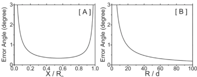
Fig. 2. The error range obtained by MTA tests, selecting only one
contour plane in the certain flux rope model. The error is defined as the angle between the modelzaxis and the MTA resulting axial orientation. (a) The error as a function ofX (the constellation’s closest distance to the axis, normalized to flux rope radiusR), when
Ris 50 times greater than the satellites’ separationd. (b) The error versus flux rope radiusR (normalized tod) in a certain type of Cluster trajectory withXto be 0.707R.
where the constellation traverses the flux rope. As an error estimation, a set of MTA tests are performed to calculate the error range by calculating the angle between the modelzaxis and the MTA result. For simplicity, the cross section of the flux rope is assumed to be circular with a radius ofR, the 4-spacecraft Cluster formation to be a regular tetrahedron with a distance of d between each two satellites, and we select only one contour plane in each of the tests to obtain the flux rope orientation as the cross product of the two normals. It is found that the error depends not only on the flux rope ra-dius, but also on the path that the satellites pass through the structure. The error dependencies on bothRand the Cluster passing path (characterized by the closest distanceX from the constellation to the axis) are clearly displayed in Fig. 2.
Figure 2a shows the resulting MTA error as a function of X (normalized by R), in the typical case of the flux rope radiusR being 50 times as d. It can be seen that the er-ror angle is very small (less than 3 deg) in the region of 0.04R<X<0.98R. For thoseX>0.98Rcases, the relatively larger error can be naturally understood to be caused by the constellation’s skimming motion over the flux rope, however, the error for thoseX<0.04R cases is a bit more amazing. Actually, in the cases when the satellites almost pass through the axis of the flux rope, the two normal directions obtained at the positions ofP1andP2are almost parallel, so that the cross product process may become invalid, leading to unex-pected errors. However, if we select more contour planes in these cases, the resulting minimum eigenvalueλ3should be very close to the intermediate one,λ2, indicating the approxi-mate parallelism of all these normal directions, and providing a warning of the invalidation of the MTA technique in those cases.
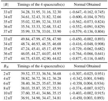
Table 1. The results of the Triangulation method as the first step
of MTA:|B|orBN selected as the signals, timings input and the
normals obtained.
|B| Timings of the 4 spacecrafts(s) Normal Obtained
33 nT 34.28, 31.95, 31.16, 32.30 (–0.647,–0.162, 0.745) 34 nT 34.61, 32.43, 31.82, 32.66 (–0.600,–0.104, 0.793) 35 nT 35.02, 32.89, 32.34, 33.03 (–0.562,–0.073, 0.824) 36 nT 35.54, 33.33, 32.68, 33.42 (–0.552,–0.091, 0.829) 37 nT 35.99, 33.78, 33.01, 33.90 (–0.579,–0.136, 0.804)
33 nT 49.84, 47.99, 47.58, 47.90 (–0.450,–0.002, 0.893) 34 nT 48.74, 46.93, 46.35, 46.68 (–0.416,–0.048, 0.908) 35 nT 47.24, 45.41, 45.17, 45.99 (–0.729,–0.062, 0.682) 36 nT 46.05, 44.27, 44.07, 44.93 (–0.764,–0.066, 0.641) 37 nT 44.75, 43.05, 42.90, 44.02 (–0.877,–0.116, 0.465)
BN Timings of the 4 spacecrafts(s) Normal Obtained
2 nT 39.52, 37.33, 36.54, 36.68 (–0.307,–0.025, 0.951) 4 nT 38.82, 36.72, 36.12, 36.28 (–0.342, 0.001, 0.940) 6 nT 38.40, 36.25, 35.67, 35.86 (–0.358, 0.004, 0.934) 8 nT 38.03, 35.87, 35.27, 35.51 (–0.374,–0.007, 0.927) 10 nT 37.60, 35.41, 34.86, 35.15 (–0.403,–0.002, 0.915) 12 nT 36.91, 34.90, 34.47, 34.81 (–0.450, 0.003, 0.893)
satellites’ separation distanced as the prediction, with the error angle less than 3 deg in the case ofRgreater than 6.1d. As a comparison with previous methods, we may have a look at the error range produced by other techniques. Xiao et al. (2004) concluded that the errors of PAA and CMVA are strongly dependent on models and the satellite paths, with a typical error of around 15−20 deg. The possible error range of the MDD technique was also tested (Shi et al., 2005), us-ing the flux rope model by Elphic and Russell (1983). They drew the conclusion that the angle between the calculated axis and the real axis is mostly less than 5 deg, providing a similar precision with the MTA technique. So, theoretical speaking, the MTA method, along with the MDD technique, may have the ability to measure the axial orientation of a certain flux rope more accurately than the traditional MVA-based methods. In order to estimate their precision beyond a theoretical point of view, it is interesting to apply the method to a real Cluster event, as will be done in the following sec-tion.
3 Applications
On 26 January 2001, several flux rope events were ob-served by Cluster satellites (e.g. Phan et al., 2004; Pu et al., 2005) when they were traveling outbound in the northern high-latitude regions from the magnetosphere to the magne-tosheath, with the spacecraft separation of∼600 km. Three of those flux rope orientations obtained by MDD analysis were calculated and listed in Table 1 of Shi et al. (2005).
24 28 32 36 40 44 48 52 28
30 32 34 36 38 40 42
Time (Second)
B total
(nT)
24 28 32 36 40 44 48 52 −15
−10 −5 0 5 10 15 20
Time (Second)
B N
(nT)
C1 C2 C3 C4
Fig. 3. A flux rope structure observed by FGM/Cluster on 26
Jan-uary 2001, 11:10:24 UT to 11:10:52 UT. (Left panel) Magnetic strength, (right panel)BNcomponents, as a function of time (both
4-s sliding averages at 0.2-s resolution).
As a comparison, the MTA technique is applied to ana-lyze these flux ropes, using magnetic field data (FGM data) (Balogh et al., 1997). One of the events, in the time inter-val of 11:10:24 UT–11:10:52 UT, is shown in Fig. 3: the left panel represents the magnetic magnitude |B| and the right panel is the N component of the magnetic fieldBN. The N
direction, being calculated as(0.63,0.33,0.70)by Pu et al. (2005), using minimum variance analysis, can be considered as the normal direction of the magnetopause during this time period. The|B|enhancement, along with the bipolar signa-ture of BN, clearly indicates a flux rope structure (Russell
and Elphic, 1978).
In order to eliminate the undesirable high-frequency fluc-tuations in applying the Triangulation method (as the first step of MTA), a procedure of a sliding average is required (Haaland et al., 2004a). Here we use a sliding window of 4 s, with a time resolution of 0.2 s, and a apply linear interpola-tion between each two consecutive measurements.
Then we can select five magnetic field values (33 nT, 34 nT, 35 nT, 36 nT and 37 nT) as the signals, shown as ma-genta dashed lines in the left panel of Fig. 3, and correspond-ingly obtain 10 normal directions (5 for arriving and 5 for departure) using the timing method. The 10 directions, listed in the upper panel of Table 1, thus lead us to the calculation of three eigenvalues and their corresponding three eigenvec-tors. The eigenvector(−0.136,0.991,0.002)with the small-est eigenvalue (λ2/λ3=21.7) should be, in principle, perpen-dicular to all of the 10 normals, and could thus be treated as the estimated flux rope orientation.
−1 −0.5 0 0.5 1
−1 −0.5 0 0.5 1 −1
−0.5 0 0.5 1
Y X
Z
−1 −0.5 0 0.5 1
−1 −0.5 0 0.5 1 −1
−0.5 0 0.5 1
Y X
Z
Fig. 4. The MTA analysis on the flux rope event during 11:10:24 UT
to 11:10:52 UT. In the left box, the magnetic strength is selected as the signal, while in the right one, theBN component is selected.
In either of the boxes, the blue lines show the normal directions obtained by the Triangulation method as the first step of MTA, and the red lines are the three eigenvectors of the corresponding matrix. The green circle represents the cross-section plane of the flux rope, basically containing all of the blue lines, while the red line which is perpendicular to the green circle suggests the flux rope orientation.
treated as the cross-section plane of the flux rope, and ba-sically contain all of the 10 normals. The third red line, (−0.136,0.991,0.002), being treated as the orientation of the flux rope, can be clearly seen to be perpendicular to the cross-section plane (and therefore to the 10 normals).
Based on the 2-D property of the flux rope model, the gra-dient ofBNwould also be within the cross-section plane. So
the normal directions of all theBN contour planes are also
perpendicular to the flux rope orientation. Therefore, we can selectBN as the signal (instead of|B|) to perform the MTA
technique, as another test of MTA validity. SixBN are
se-lected (2 nT, 4 nT, 6 nT, 8 nT, 10 nT and 12 nT), also shown as magenta dashed lines in the right panel of Fig. 3, and the resulting normals are listed in the bottom panel of Table 1.
The six normals, along with the three corresponding eigen-vectors, are shown in the right GSE box of Fig. 4, with the same format as the left one. Although they are shown to be very close to each other, they are still well confined in a plane with the normal to be(0.117,0.992,0.051). This direction, also being treated as the flux rope orientation, is pretty sim-ilar to the one calculated before, which in some sense con-firms the reliability and consistency of the MTA technique.
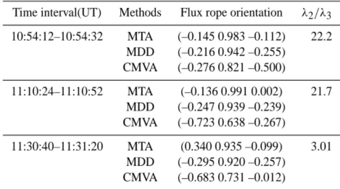
The other two events listed in Shi et al. (2005) are also re-calculated using the MTA technique, shown in Table 2, along with the one we displayed before. Hereλ2andλ3denote the intermediate and minimum eigenvalues of MTA, suggesting the third rowλ2/λ3to be an indicator of the MTA estimating precision. As a comparison, the resulting orientations ob-tained by some other methods, including MDD and CMVA, are also listed.
It can be clearly seen that the directions calculated by MTA technique are pretty close to those obtained by MDD, with a deviation between them of around 10 deg. The
sim-Table 2. MTA results of three flux ropes observed on 26 January
2001, along with the comparison with other methods.
Time interval(UT) Methods Flux rope orientation λ2/λ3
10:54:12–10:54:32 MTA (–0.145 0.983 –0.112) 22.2 MDD (–0.216 0.942 –0.255) CMVA (–0.276 0.821 –0.500)
11:10:24–11:10:52 MTA (–0.136 0.991 0.002) 21.7 MDD (–0.247 0.939 –0.239) CMVA (–0.723 0.638 –0.267)
11:30:40–11:31:20 MTA (0.340 0.935 –0.099) 3.01 MDD (–0.295 0.920 –0.257) CMVA (–0.683 0.731 –0.012)
ilarity between them thus suggests the validity of the MTA method.
On the other hand, the CMVA results show relatively larger deviations, especially in the second and third cases. This is mainly caused by the error produced in the calcula-tion of electric current. The typical| ▽ ·B|/| ▽ ×B|value of∼0.4, indicating the inaccuracy of the electric current ob-tained, might strongly reduce the reliability of the CMVA method in these cases.
It should also be pointed out that the value ofλ2/λ3 is as small as 3.01 in the last case, implying an uncertainty in determining the flux rope orientation. The uncertainty can be probably explained by the traversing path of Cluster to be too close to the flux rope center. Actually, in this case, the resulting deviations between MTA and MDD are relatively larger than the other two.
4 Conclusions
We have introduced another method called the MTA tech-nique, to find out the axial orientation of a certain flux rope by a 4-spacecraft constellation. Basically, the error range of the MTA technique critically depends on both the satel-lite separation distance and the constellation path via the flux rope. In spite of these, the MTA has proved itself to be an ac-curate method in a theoretical way. Also, the Cluster data has been used as an application of the MTA technique. Selecting both|B|andBNas the signal, similar resulting orientations
Appendix A
Error estimation for random errors
The random errors ofN(m), either caused by the measure-ment inaccuracy or by the quantization effects of the Trian-gulation method, can be treated as a set of errors being in-dependent from each other and having identical probability distributions (independent, identical distributions, denoted as iid), which satisfy the assumption in Khrabrov and Sonnerup (1998a) (hereinafter as paper 1). Within this framework, the data series appear as one of the possible fluctuating states of the normal vector pattern.
So we can directly follow the procedure of paper 1, how-ever, we do not mean to repeat the lengthy manipulations. Instead, we will mainly emphasize the difference between them, to obtain the final result of the MTA error range.
The minimization method applied in MTA would produce a symmetric matrix
Lµν = hNµ(m)Nν(m)i
in comparison with the matrix in MVA Mµν = hBµ(m)Bν(m)i − hBµ(m)ihBν(m)i,
where the bracketsh irepresent the averaging process over the measured data set.
Note that another averaging operation, denoted by double bracketshh ii, means the average over the ensemble of all possible fluctuating states. And certainly the ensemble aver-age,hh ii, and the average over the data in a given state,h i, can be interchanged, i.e.h[hh ii]i = hh[h i]ii.
In order to depict a certain fluctuating state, the vector
N(m) can be expressed asN∗(m)+n(m), where the asterisk
means the signal andnis the noise with an iid distribution. Some properties of the iid distribution can be listed below:
hhn(m)ii =0, m=1,2...M . (A1) Equation (4) of paper 1 suggests that the mean value of the errors is zero, if taken over all of the fluctuating states. Another property is the one in Eq. (5) of paper 1:
hhn(m)µ n(k)ν ii ≡Sµνδmk, (A2)
where Sµν is independent of m andk, and stands for the
second-order terms of the noise.
Now the symmetric matrixLµνcan be turned to
Lµν = h(Nµ∗(m)+nµ(m))(Nν∗(m)+n(m)ν )i
=L∗µν+hn(m)µ n(m)ν i+hn(m)µ Nν∗(m)i+hNµ∗(m)n(m)ν i. (A3) Then the ensemble average can be taken on both sides. Based on the properties of Eqs. (A1) and (A2), the last two terms in the right sides of Eq. (A3) can be neglected:
hhLµνii =L∗µν+ hh[hn(m)µ n(m)ν i]ii =L∗µν+Sµν (A4)
which would replace Eq. (8) of paper 1 in our procedure, and Eq. (11) of paper 1 would be correspondingly switch to L∗ij+Sij =δijhhλiii (A5)
in the coordinate system ofhhLiieigenbasis, and the compo-nents would be denoted by the subscriptsiandj.
The next step would be connecting the fluctuations of eigenvectorsxi and eigenvalues λi to the noise in a given
fluctuating state, by linearizing the eigenproblem. As is shown in paper 1 (Eq. 12), the component of 1xi along
hhxjiican be expressed as:
1xij = −1xj i =
1Lij hhλiii − hhλjii
i6=j (A6)
which suggests the role of the certain fluctuating state, rotat-ingxiat an angle of1xij towardxj, in radians.
So, in order to obtain the angular error of the MTA eigen-vectors, the variance of L should be first calculated as the following:
hh(1Lij)2ii ≡ hh(Lij− hhLijii)2ii
= hh{ 1
M
M
X
m=1
(Ni∗(m)+n(m)i )(Nj∗(m)+n(m)j )
−1
M
M
X
k=1
(Ni∗(k)Nj∗(k)+ hhninjii)}2ii. (A7)
Equation (A7) can be expressed as the sum of a set of terms, each of which is proportional to the first, second, third and fourth moment ofn. As we know from Eq. (A1), the first or-der terms have the value of zero. Furthermore, if we assume that the noise is smaller than the signal, the third and fourth terms can be also neglected. Equations (A2) and (A4) can be used in the next manipulation, and Eq. (A7) turns to:
hh(1Lij)2ii =
1 M(L
∗
iiSjj+L∗jjSii+2L∗ijSij) . (A8)
The combination of Eq. (A6) and Eq. (A8) thus leads to the angular error of the eigenvectors:
1φij ≡
q
hh(1xij)2ii =
s
hh(1Lij)2ii
(hhλiii − hhλjii)2
=
s
L∗iiSjj+L∗jjSii+2L∗ijSij
M(hhλiii − hhλjii)2
. (A9)
Consider Eq. (A5) and neglect the higher order terms, Eq. (A9) turns to:
1φij =
s
hhλiiiSjj+ hhλjiiSii
M(hhλiii − hhλjii)2
. (A10)
Specifyingi=3 withj=1 or 2, and based on the fact that the eigenvalueλ3is entirely due to the noise, Eq. (A10) then becomes
1φ3j =
s
λ3λj
M(λ3−λj)2
In arriving at this result,S33is replaced byλ3and we fur-ther assumeSjj to also be of order ofλ3, so thatλ3Sjjwould
be of a higher order and could be thus neglected, (see paper 1 for more detail).
So the random angular errors of the MTA flux rope orien-tation can be obtained, as the function of the three eigenval-ues and also the number of normal vectors.
Acknowledgements. The authors thank H. Zhang and C.-J. Xiao for many helpful discussions. This work is supported by NSFC project 40390152 and 40528005. The research was initiated during a visit by X.-Z. Zhou to Boston University in Fall/Winter 2004, sup-ported by NASA grant NAG5-10108.
Topical Editor I. A. Daglis thanks C. J. Farrugia and another referee for their help in evaluating this paper.
References
Balogh, A., Dunlop, M. W., Cowley, S. W. H., Southwood, D. J., Thomlinson, J. G., Glassmeier, K.-H., Musmann, G., L¨uhr, H., Buchert, S., Acu˜na, M. H., Fairfield, D. H., Slavin, J. A., Riedler, W., Sachwingenschuh, K., and Kivelson, M. G.: The Cluster Magnetic Field Investigation, Space Sci. Rev., 79, 65–91, 1997. Dunlop, M. W., Southwood, D. J., Glassmeier, K. H., and Neubauer,
F. M.: Analysis of multipoint magnetometer data, Adv. Space Res., 8(9), 273–277, 1988.
Elphic, R. C. and Russell, C. T.: Magnetic Flux ropes in the Venus ionosphere: Observations and models, J. Geophys. Res., 88, 58– 72, 1983.
Elphic, R. C. and Southwood, D. J.: Simultaneous measurements of the magnetopause and flux transfer events at widely separated sites by AMPTE UKS and ISEE 1 and 2, J. Geophys. Res., 92, 13 666–13 672, 1987.
Farrugia, C. J., Elphic, R. C., Southwood, D. J., and Cowley, S. W. H.: Field and flow perturbations outside the reconnected field region in flux transfer events: Theory, Planet. Space Sci., 35(2), 227–240, 1987.
Haaland, S., Sonnerup, B. U. O., Dunlop, M. W., Balogh, A., Georgescu, E., Hasegawa, H., Klecker, B., Paschmann, G., Puhl-Quinn, P., R`eme, H., Vaith, H., and Vaivads, A.: Four-spacecraft determination of magnetopause orientation, motion and thick-ness: comparison with results from single-spacecraft methods, Ann. Geophys., 22, 1347–1365, 2004a.
Haaland, S., Sonnerup, B. U. O., Dunlop, M. W., Georgescu, E., Paschmann, G., Klecker, B., and Vaivads, A.: Orientation and motion of a discontinuity from Cluster curlometer capability: Minimum variance of current density, Geophys. Res. Lett., 31, L10 804, doi:10.1029/2004GL020,001, 2004b.
Hau, L. N. and Sonnerup, B. U. O.: Two-dimensional coherent structures in the magnetopause: Recovery of static equilibria from single-spacecraft data, J. Geophys. Res., 104, 6899–6918, 1999.
Hu, Q. and Sonnerup, B. U. O.: Reconstruction of magnetic clouds in the solar wind: Orientations and configurations, J. Geophys. Res., 107 (A7), doi:10.1029/2001JA000293, 2002.
Khrabrov, A. V. and Sonnerup, B. U. O.: Error estimates for min-imum variance analysis, J. Geophys. Res., 103, 6641–6651, 1998a.
Khrabrov, A. V. and Sonnerup, B. U. O.: Orientation and motion of current layers: Minimization of the Faraday residue, J. Geophys. Res., 25, 2373–2376, 1998b.
Lepping, R. P., Jones, J. A., and Burgala, L. F.: Magnetic field struc-ture of interplanetary magnetic clouds at 1 AU, J. Geophys. Res., 95, 11 957–11 965, 1990.
Phan, T. D., Dunlop, M. W., Paschmann, G., Klecker, B., Bosqued, J. M., R`eme, H., Balogh, A., Twitty, C., Mozer, F. S., Carlson, C. W., Mouikis, C., and Kistler, L. M.: Cluster observations of continuous reconnection at the magnetopause under steady inter-planetary magnetic field conditions, Ann. Geophys., 22, 2355– 2367, 2004.
Pu, Z. Y., Zong, Q. G., Fritz, T. A., Xiao, C. J., Huang, Z. Y., Fu, S. Y., Shi, Q. Q., Dunlop, M. W., Glassmeier, K. H., Balogh, A., Daly, P., R`eme, H., Dandouras, J., Cao, J. B., Liu, Z. X., Shen, C., and Shi, J. K.: Multipule flux rope events at the high-latitude magnetopause: Cluster/Rapid observation on January 26, 2001, in: The Magnetospheric Cusps: Structure and Dynamics, edited by Fritz, T. A. and Fung, S. F., Springer, Netherlands, 191–212, 2005.
Russell, C. T. and Elphic, R. C.: Initial ISEE magnetometer results: Magnetopause observations, Space Sci. Rev., 22, 681–715, 1978. Russell, C. T., Mellott, M. M., Smith, E. J., and King, J. H.: Mul-tiple Spacecraft Observations of Interplanetary Shocks: Four Spacecraft Determination of Shock Normals, J. Geophys. Res., 88, 4739–4748, 1983.
Shi, Q. Q., Shen, C., Pu, Z. Y., Dunlop, M. W., Zong, Q.-G., Zhang, H., Xiao, C. J., Liu, Z. X., and Balogh, A.: Dimensional analysis of observed structures using multi-point magnetic field measure-ments: Application to Cluster, Geophys. Res. Lett., 32, L12 105, doi:10.1029/2005GL022454, 2005.
Siscoe, G. L., Davis Jr., L., Coleman Jr., P. J., Smith, E. J., and Jones, D. E.: Power Spectra and Discontinuities of the Interplan-etary Magnetic Field: Mariner 4, J. Geophys. Res., 73, 61–82, 1968.
Sonnerup, B. U. O. and Cahill Jr., L. J.: Explorer 12 Observations of Magnetopause Current Layer, J. Geophys. Res., 73, 1757–1771, 1968.
Sonnerup, B. U. O. and Scheible, M.: Minimum and Maximum Variance Analysis, in: Analysis Methods for Multi-spacecraft Data, edited by: Paschmann, G. and Daly, P., ISSI/ESA, Nether-lands, 185–220, 1998.
Sonnerup, B. U. O., Haaland, S., Paschmann, G., Lavraud, B., Dun-lop, M. W., R`eme, H., and Balogh, A.: Orientation and motion of a discontinuity from single-spacecraft measurements of plasma velocity and density: Minimum mass flux residue, J. Geophys. Res., 109, A03 221, doi:10.1029/2003JA010230, 2004. Xiao, C. J., Pu, Z. Y., Ma, Z. W., Fu, S. Y., Huang, Z. Y., and
Zong, Q. G.: Inferring of flux rope orientation with the minimum variance analysis technique, J. Geophys. Res., 109, A11 218, doi:10.1029/2004JA010594, 2004.