A Hybrid Approach for Assessments of Equivalent Emission Sources and Electromagnetic Environments

(1)

Brazilian Microwave and Optoelectronics Society-SBMO received 18 Sep 2017; for review 18 Sep 2017; accepted 14 Dec 2017

Abstract—_{This paper presents a method for equivalent emission} source determination by application of LLAs (Large Loop Antennas). A review of different types of LLAs is carried out and their characteristics regarding emission source evaluation are emphasized. A hybrid technic is applied for obtaining the electric fields based on previous measurement of magnetic fields combined with an analytical and numerical approach. This methodology is proposed as an alternative to face the constraints concerning to the near electric fields measurements and calculations.

Index Terms—_{Theoretical and Numerical Methods, Field Measurements,}

Large Loop Antennas, Equivalent Emission Sources, Near Field Calculation.

I. INTRODUCTION

The technological advancements bring to the society an immense quantity of benefits, as: modern

communication systems, comfort, transportation, etc. However, additionally, it leads to an

increasingly congested electromagnetic environment. Historically, the effects of exposition to

electromagnetic fields are being intensively discussed, in order to determine the acceptable limits of

the fields emitted by a certain source or supported by an electric or electronic device (immunity). For

certain areas of engineering, as automotive, the electromagnetic emission limits are referenced by

several standards that regulate the well known electromagnetic compatibility (EMC) tests [1], [2].

The electromagnetic fields measurement in anechoic or shielded chambers is the most usual technic

applied for radiated EMC evaluation. Nevertheless, this technic requires a large quantity of equipment

and infrastructure. Additionally, this technic requires a real (physical) model of the device that will be

tested, which is usually available only in intermediate phases of design. It means that, in case of a test

reproval and consequent re-design, a large amount of funding is necessary, because of the spending

with new prototypes and re-tests.

In this mean, hybrid methods using measurements, analytical and numerical calculation can be

suitable for supporting EMC evaluations in earlier phases of a device design and allowing a larger

number of models to be tested and optimized.

During the last years, Large Loop Antennas are being intensively studied as a method of

measurement of electric and electronic devices. Alternatively, this type of antenna allows the

determination of the equivalent emission source, when the right technics are applied. These technics

A Hybrid Approach for Assessments of

Equivalent Emission Sources and

Electromagnetic Environments

D. V. F. Cardia1, C. A. F. Sartori1,2, R. P. B. Muylaert1

1_{PEA/EPUSP - Escola Politécnica da Universidade de São Paulo, Departamento de Engenharia Elétrica} 2

(2)

are described in [3]-[9].

The equivalent emission sources may be represented, as a first approach, by magnetic and electric

dipoles that can be determined through the application of van Veen and Bergervöt Antenna, Kanda

Antenna or Multipole Antenna.

The measurement of the magnetic dipole is normally carried out, since these antennas’

measurements happen in the near field region, where the magnetic fields are much more

representative than electric fields [7]. Especially in some cases, the measurement of electric fields

cannot be precisely performed [10].

On the other hand, as can be verified on EMC Standards, as [1] and [2], the emission limits are

represented by electric fields, in most of the cases. Thus, it is important to obtain the electric fields

emitted by an arbitrary source, in order to check the whole electromagnetic scenario. To overcome

this gap, a hybrid technic is proposed to calculate the electric fields from the magnetic fields, based on

measurements and Analytical/FDTD calculation method [10].

II. OBTAININGEQUIVALENTEMISSIONSOURCESBYLLAS

As already mentioned, some types of LLA are being studied for obtaining equivalent emission

sources. The most known of them are: van Veen and Bergervöt Antenna, Kanda Antenna and

Multipole Antenna. All of these antennas have some common characteristics, being composed by

large loops, that surrounds the Device Under Test (DUT). The electric currents measured in these

loops are induced by the electromagnetic fields emitted by the DUT. From these measured currents

and with the right technics applied, the DUT’s equivalent emission source is obtained.

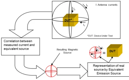
The general process for obtaining the equivalent emission sources, is shown below, in Fig, 1.

Fig. 1. DUT to Equivalent Emission Source transformation process by LLA measurement

From the picture above, the current of the magnetic dipole (in) is calculated from the current

measured in loop (In), for n = x, y and z. However, the total DUT representation shall be composed by

the three magnetic dipoles supplied by currents ix, iy and iz.

It is briefly described how to obtain the equivalent emission source with the application of main

(3)

Brazilian Microwave and Optoelectronics Society-SBMO received 18 Sep 2017; for review 18 Sep 2017; accepted 14 Dec 2017 A. The van Veen and Bergervöt Antenna

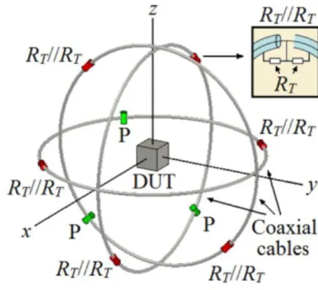
The van Veen and Bergervöt Antenna is represented in Fig. 2 [5].

Fig. 2. The van Veen and Bergervöt Antenna Representation

This antenna is composed by three large loops, orthogonally disposed, assembled with coaxial

cables. The current measurement is made on “P” points, shown in the picture above, directly with a

current probe. The representation of the DUT measured by this antenna is only possible by magnetic

dipoles, so it does not have capacity of electric dipoles representation and multipole “filtering” (3rd

order element – octupole – influences in dipole measurement) [7].

The DUT is placed inside this antenna, generating a current IPn that is the current measured in the

point “P” of each loop. Each loop is represented by the index n = x, y or z. The induced current IAn is calculated by:

𝐼𝐴𝑛 = 𝐼𝑃𝑛

{ 𝑅𝐶 𝑅𝑇𝑠𝑒𝑛 (

𝑘𝐶π𝑏

2 ) + jcos ( 𝑘𝐶π𝑏

2 ) +

+j2π𝑅_{μc [ln (}𝐶 8𝑏_𝑎𝐶) − 2]−1𝑠𝑒𝑛 (𝑘 𝐶π𝑏

2 ) tan (𝑘π𝑏_{2 ) }}

(1)

Where IPn is the measured current, RC is the coaxial cable characteristic impedance, RT is the

termination impedance, kc is the propagation constant, µ is the magnetic permeability, ac is the coaxial

cable sectional radius and b is the large loop radius.

As detailed in [6], the magnetic dipole current (in), is so obtained by:

𝑖𝑛=𝐼𝐴𝑛2𝑏𝐿𝐴

μ0π𝑞2 (2)

The current in, where n = x, y or z, shall be applied to the three magnetic dipoles that composes the

equivalent emission source, as shown in figure 1.

This current only refers to the magnetic component of the DUT’s emission. The electric component

(4)

Brazilian Microwave and Optoelectronics Society-SBMO received 18 Sep 2017; for review 18 Sep 2017; accepted 14 Dec 2017 B. The Kanda Antenna

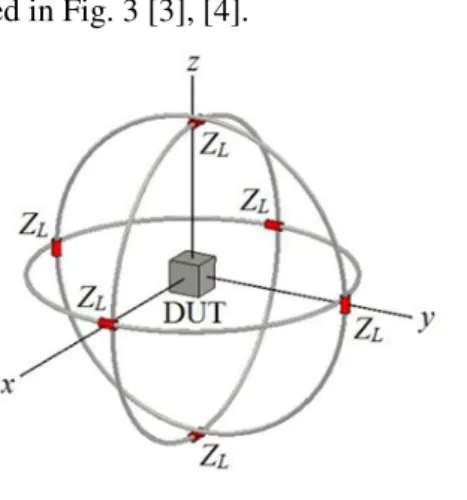
The Kanda Antenna is represented in Fig. 3 [3], [4].

Fig. 3. Kanda Antenna Representation

This antenna is composed by three large loops, orthogonally disposed, assembled with rigid wires

or curved metallic pipes. It requires external processing for total measured current in each loop, what

adds a difficulty on its application. It has the capacity of DUT representation by magnetic dipole

and/or electric dipole, but does not have capacity of multipole “filtering” (3rd order element – octupole

– influences in dipole measurement).

To obtain the magnetic dipole, the DUT is placed inside this antenna, resulting on I∑n, that is the

sum of the currents measured in the points “0” (I0n) and “π” (Iπn) of each loop. Each loop is represented by the index n = x, y or z.

𝐼Σ_𝑛 =𝐼0𝑛+ 𝐼π𝑛

2 =

2π𝑏𝑚𝑀_𝑛𝐺𝑀𝑌0

1 + 2𝑌0𝑍𝐿 (3)

With some mathematical arrangements [3], [4] the magnetic moment of the magnetic dipole can be

obtained by:

𝑚𝑀𝑛= 2𝐼Σ𝑛

jη𝑘𝑏[ln(8𝑏 𝑎⁄ ) − 2] + 2𝑍𝐿

η𝑘2_{[1 + 1 (j𝑘𝑏)}_⁄ _]𝑒−j𝑘𝑏 (4)

Finally the magnetic dipoles currents, for each one of the three loops, are obtained by:

𝑖𝑛=𝑚𝑀𝑛

π𝑞2 (5)

The current of each magnetic dipole here is obtained with regards only to the magnetic moment of

the measurement. Similarly, an additional part, related to the electric moment, can be obtained by IΔn

calculation [3], [4].

In order to keep similarity with the DUT’s representation by van Veen and Bergervöt Antenna,

which can only obtain the magnetic part, the electric part is disregarded.

C. The Multipolar Antenna

(5)

Source: S. Zangui [8]

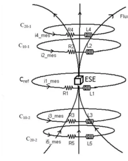
Fig. 4. Multipolar Antenna Representation

This antenna is composed by large loops, concentrically disposed, forming a sphere. It is assembled

with rigid wires. The current is measured directly on the loop without necessity of external

processing. The DUT is represented by magnetic multipoles. It has the capacity of multipole

“filtering” (separate measurement for 1st

and 2nd orders elements).

For the magnetic dipole obtaining, the DUT is measured in this antenna, resulting on coefficient

A10, as follows:

𝐴10=10 8_𝑟

𝑀

32π (ϕ10_1− ϕ10_2) = 2,24.105(ϕ10_1− ϕ10_2) (6)

Where rM is the antenna’s sphere radius and ϕ10_n is the magnetic flux of the C10_n loop.

The flux is calculated from the measured current (I), by:

ϕ10_𝑛= 𝐼10_𝑛. 𝐿 (7)

Where L is the loop inductance, that is obtained by:

𝐿 = μ0𝑏 (ln (8𝑏_𝑟 𝑐) −

7

4) (8)

Finally, to obtain the current for each loop that represents the DUT:

𝑖𝑛=π𝑟_𝐴102 (9)

D. Electromagnetic Fields Analytical Calculation

With the currents measured by any of the antennas mentioned above, the magnetic dipole can be

determined (with calculated currents ix, iy and iz, for each loop as in fig. 1). Single loop is represented

(6)

Brazilian Microwave and Optoelectronics Society-SBMO received 18 Sep 2017; for review 18 Sep 2017; accepted 14 Dec 2017 Fig. 5. Electromagnetic Fields Emitted by a Magnetic Dipole

And the fields can be calculated by, for each single loop (in spherical coordinates) [11]:

𝐻𝑟= 𝑗𝑘𝑞2_2𝑟𝑖𝑐𝑜𝑠𝜃₂ (1 +_{𝑗𝑘𝑟) 𝑒}1 −𝑗𝑘𝑟 (10)

𝐻𝜃= −(𝑘𝑞)_4𝑟2𝑖𝑠𝑒𝑛𝜃(1 +_{𝑗𝑘𝑟 −}1 _(𝑘𝑟)1 ₂) 𝑒−𝑗𝑘𝑟 (11)

𝐻ϕ= 0 (12)

𝐸𝑟= 𝐸θ= 0 (13)

𝐸ϕ= η𝑗(𝑘𝑞) 2_{𝑖𝑠𝑒𝑛θ}

4𝑟 (1 +

1 𝑗𝑘𝑟) 𝑒−𝑗𝑘𝑟

(14)

Converting to rectangular coordinates:

𝐻𝑥= 𝑠𝑒𝑛θcosϕ𝐻𝑟+ cosθcosϕ𝐻θ− 𝑠𝑒𝑛ϕ𝐻ϕ 𝐻𝑦= 𝑠𝑒𝑛θ𝑠𝑒𝑛ϕ𝐻𝑟+ cosθ𝑠𝑒𝑛ϕ𝐻θ+ cosϕ𝐻ϕ 𝐻𝑧= cosθ𝐻𝑟− 𝑠𝑒𝑛θ𝐻θ

(15)

𝐸𝑥= 𝑠𝑒𝑛θcosϕ𝐸𝑟+ cosθcosϕ𝐸θ− 𝑠𝑒𝑛ϕ𝐸ϕ 𝐸𝑦= 𝑠𝑒𝑛θ𝑠𝑒𝑛ϕ𝐸𝑟+ cosθ𝑠𝑒𝑛ϕ𝐸θ+ cosϕ𝐸ϕ 𝐸𝑧= cosθ𝐸𝑟− 𝑠𝑒𝑛θ𝐸θ

(16)

E. Analytical/FDTD Hybrid Method for Electric Field calculation

As an alternative to the aforementioned analytical calculation, this hybrid method is presented.

From [10] this method has been proposed, specifically for electric fields calculation, from

atmospheric discharges.

As a great contribution, this method allows the calculation of the electric fields (E) from the

magnetic flow density vector (B) that can be obtained by measurements and analytical or numerical

calculations.

(7)

Source: C. Sartori and J. Cardoso [10]

Fig. 6. Representation of electrical fields obtaining from magnetic flow density vectors

The magnetic flow density vector (B) in each point of space shall be calculated from the magnetic

field (H) emitted by a magnetic dipole, which can be calculated analytically (equations (10), (11), (12)

and (15)). B is obtained by:

𝐵⃗ 𝑛= 𝐻𝑛μ (17)

For one point of space, Ex, Ey and Ez, are calculated from components B around to this point.

Also, the distance between these points (δl) is important for this method, calculated by :

δ𝑙 ≤ 0,01𝑅 (18)

Where, R is the distance from the DUT’s center to the chosen measurement point on space.

𝑘 +1_{2 𝐸}𝑧(𝑚, 𝑛, 𝑝)

= 𝑘 −1_{2 𝐸}𝑧(𝑚, 𝑛, 𝑝) +𝑐2_{δ𝑙 [𝑘𝐵}Δ𝑡 𝑦(𝑚, 𝑛 + 1, 𝑝)

−𝑘𝐵𝑦(𝑚, 𝑛 − 1, 𝑝) + 𝑘𝐵𝑥(𝑚, 𝑛, 𝑝 − 1) − 𝑘𝐵𝑦(𝑚, 𝑛, 𝑝 + 1)]

(19)

𝑘 +1_{2 𝐸}𝑥(𝑚, 𝑛, 𝑝)

= 𝑘 −1_{2 𝐸}𝑥(𝑚, 𝑛, 𝑝) +𝑐 2_Δ𝑡

δ𝑙 [𝑘𝐵𝑧(𝑚, 𝑛, 𝑝 + 1)

−𝑘𝐵𝑧(𝑚, 𝑛, 𝑝 − 1) + 𝑘𝐵𝑦(𝑚 − 1, 𝑛, 𝑝) − 𝑘𝐵𝑦(𝑚 + 1, 𝑛, 𝑝)]

(20)

𝑘 +1_{2 𝐸}𝑦(𝑚, 𝑛, 𝑝)

= 𝑘 −1_{2 𝐸}𝑦(𝑚, 𝑛, 𝑝) +𝑐2_δ𝑙Δ𝑡[𝑘𝐵𝑥(𝑚 + 1, 𝑛, 𝑝)

−𝑘𝐵𝑥(𝑚 − 1, 𝑛, 𝑝) + 𝑘𝐵𝑧(𝑚, 𝑛 − 1, 𝑝) − 𝑘𝐵𝑧(𝑚, 𝑛 + 1, 𝑝)]

(8)

The time-step factor "k" shall be defined by:

Δ𝑡 ≤_2𝑐δ𝑙 (22)

With these parameters, a mathematical tool may be used to calculate it, with time-steps processing.

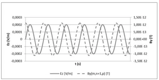
Finally, the components of electric fields are calculated (Ex, Ey and Ez). A representation of Ez

compared to By, is shown in Fig. 7.

Fig. 7. Example of electric field (Ez) resulting from calculation and comparison with magnetic flow density vector (By).

III. EXPERIMENTAL VALIDATION

In this chapter a comparison between three methods is shown: analytical method, numerical,

method and hybrid method, this last one is the focus of this paper.

The general process of experimental validation is summarized in Fig. 8, for a simpler understanding

of the process.

Fig. 8. Visual chart of experimental validation process

The first step is the equivalent magnetic dipole current obtaining, that shall be made with one of the

antennas presented in chapter II. Due to the availability and most simplified construction, the Kanda

Antenna has been utilized for the experimental validation. Originally the Kanda Antenna is composed

by 3-loop, orthogonally disposed, as shown before. But only one loop is considered, and,

conceptually, it is enough for this validation. For a complete Kanda Antenna utilization, this whole

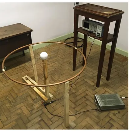
procedure should be executed three times, once for each loop, as shown in Fig. 9.

(9)

induced current from magnetic dipole (I∑) were calculated.

Fig. 9. Test setup with Kanda Antenna and a small current loop (as the DUT)

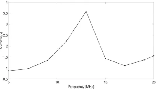
Separated currents (I0 and Iπ) were measured on terminal resistors, from 5 MHz to 20 MHz, and,

after external processing, the final induced current I∑ resulted on (as shown in chapter II-B, equation

(3)) the curve shown in Fig. 10.

Fig. 10. Kanda Antenna Current (I∑) measured and processed

From the equations (3), (4) and (5), the equivalent magnetic dipole current (ix) was obtained and

(10)

Brazilian Microwave and Optoelectronics Society-SBMO received 18 Sep 2017; for review 18 Sep 2017; accepted 14 Dec 2017 Fig. 11. Equivalent magnetic dipole current (ix) calculated

For an application with a complete Kanda Antenna, this process should be repeated, to obtain the

currents iy and iz, for the antenna loops “y” and “z”, and respective equivalent magnetic loop “y” and

“z” (see fig. 1).

From the equivalent magnetic dipole current shown above, the magnetic and electric fields emitted

by the magnetic dipole were analytically calculated in many points of space, from equations (10)-(16).

As already mentioned, the electric fields are alternatively calculated by a Hybrid Method. For that,

the magnetic flow density vector (B) was calculated from the magnetic fields (H) and from these

values it was calculated the electric fields (E).

Additionally, to enrich the comparison, two numerical models were created in a numerical

simulation tool [12]. These models have been intensively evaluated and several iterations have been

ran, in order to have the most appropriated models for this comparison, resulting in two models, one

composed by 11.000 tetrahedrons (model “a”), more simple (but faster, for computer processing) and

another one composed by 500.000 tetrahedrons (model “b”), more detailed (but much slower, for

computer processing).

Figure 12 represents both models (only the quantity of elements is different).

Fig. 12. Numerical models. Magnetic Dipole (1) and Electric Fields Probes (2)

(11)

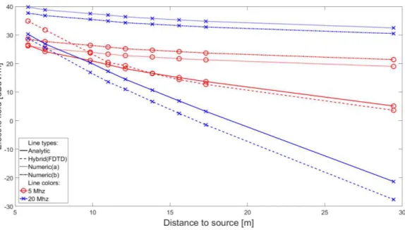
Brazilian Microwave and Optoelectronics Society-SBMO received 18 Sep 2017; for review 18 Sep 2017; accepted 14 Dec 2017 Numerical (“a” and “b” models) is shown in Fig. 13, with the results in 5 MHz and 20MHz, calculated in some points of space ranging from 5.8 meters to 29.4 meters (distances from the center

of the magnetic dipole to the measurement points).

Fig. 13. Total electric field (5 MHz and 20 MHz) calculated by analytical, hybrid and numerical methods

The same was calculated for others frequencies, ranging from 5 MHz to 20 MHz. The 3D charts

show the whole range, in Fig. 14, with analytical method, hybrid method, numerical model “a” and

numerical model “b”.

Fig. 14. 3D charts of total electric field from 5 MHz to 20 MHz calculated by analytical (1), hybrid (2) and numerical methods (“a” (3) and “b” (4) numerical models)

1 2

(12)

IV. DISCUSSION ON METHOD RESULTS

In the last chapter three different methods have been compared, analytical method, numerical

method and hybrid method, and from the results shown above, it can be emphasized that the proposed

hybrid method, when compared to analytical method, shows a good relation and precision (difference

between 0.05 to 6 dBµV/m with 0.85 dBµV/m in average). The differences in 20 MHz are bigger than

in 5 MHz, due to the dimensional characteristics of the hybrid method. By the other side, the

numerical method showed a bigger difference when compared to analytical calculation (difference

about 15 dBµV/m, in average). This result is related to the numerical modeling characteristics, as the

model shape, solver type, etc., and to the computer capacity.

However, it can be concluded that the proposed hybrid method is applicable for the electric fields

calculation.

V. CONCLUSIONS

Initially, it can be mentioned the relevance of DUT’s representation by equivalent emission sources,

as represented in this paper, considering its ease construction, lacking any complex geometry and thus

very easily represented in a simulation model.

Any of the LLAs here presented are able to be applied with this method, each one with some

different characteristics, but all of them are applicable. Multipolar Antenna represents the last status

of development for equivalent emission sources determination, since it separates the multipole

characteristics of a DUT, increasing the precision when rebuilding it by magnetic dipoles,

quadrupoles, octupoles, etc.

Regarding to the electric fields, the results obtained by the proposed hybrid method can offer a

better approximation than the ones obtained by numerical simulation modeling. Considering that the

obtaining of electric fields with a good precision is a real necessity, the application of the proposed

hybrid method shows an advance in this field of study. This method is especially useful because the

input for this method is the magnetic flow density vector, which can be obtained by measurement or

calculation, regardless of the emission source type.

However, the application of the hybrid method, together with measurements by LLAs, represents a

good and applicable method for the representation of DUTs by equivalent emission sources, in order

to allow the assessment of electromagnetic environments that can be especially suitable for

electromagnetic compatibility evaluations.

REFERENCES

[1] CISPR 25: 2008-03, Vehicles, boats and internal combustion engines - Radio disturbance characteristics - Limits and methods of measurement for the protection of on-board receivers.

[2] ISO 11452: 2005-02, Road vehicles — Component test methods for electrical disturbances from narrowband radiated electromagnetic energy.

[3] M. Kanda and D. Hill, “A three-loop method for determining the radiation characteristics of an electrically small source”, IEEE Transactions on Electromagnetic Compatibility, vol. 34, no. 1, Aug. 1992.

(13)

Brazilian Microwave and Optoelectronics Society-SBMO received 18 Sep 2017; for review 18 Sep 2017; accepted 14 Dec 2017 [5] J. R. Bergervöt and H. v. Veen, “A Large-Loop Antenna for Magnetic Field Measurements”, Zurich International

Symposium on EMC, Proceedings, 1989.

[6] D. Cardia, “Aplicação Da Antena de Van Veen E Bergervöt Na Análise De Contribuições De Fontes De Emissão Radiada Em Ambientes Eletromagnéticos”, Dissertação de Mestrado, Universidade de São Paulo, 2010.

[7] B. Vincent, “Identification de sources eletromagnétiques multipolaires équivalentes par filtrage spatial: Application à la CEM rayonée pour le convertisseurs d’eletronique de puissance”, These, L’Institut polytechnique de Grenoble, 2009. [8] S. Zangui, “Determination et Modelisation du Couplage en Champ Proche Magnetique entre Systemes Complexes”,

These, Université de Lyon, 2011.

[9] A. Bréard et al, “Overview on the Evolution of Near Magnetic Field Coupling Prediction Using Equivalent Multipole Spherical Harmonic Sources”, IEEE Transactions on Electromagnetic Compatibility, vol. 59, no. 2, pp. 584-592, 2017. [10] C. Sartori and J. Cardoso, “An Analytical-FDTD Method for Near LEMP Calculation”, IEEE Transactions on

Magnetics, vol. 36, no. 4, pp. 1631-1634, 2000.