Sensitivity analysis of runoff modeling to statistical downscaling models in the western Mediterranean

(1)

HESSD

12, 10067–10108, 2015

Sensitivity analysis of runoffmodeling to

statistical downscaling models

B. Grouillet et al.

Title Page

Abstract Introduction

Conclusions References

Tables Figures

◭ ◮

Back Close

Full Screen / Esc

Printer-friendly Version Interactive Discussion

Discussion

P

a

per

|

Discussion

P

a

per

|

Discussion

P

a

per

|

Discussion

P

a

per

|

Hydrol. Earth Syst. Sci. Discuss., 12, 10067–10108, 2015 www.hydrol-earth-syst-sci-discuss.net/12/10067/2015/ doi:10.5194/hessd-12-10067-2015

This discussion paper is/has been under review for the journal Hydrology and Earth System Sciences (HESS). Please refer to the corresponding final paper in HESS if available.

Sensitivity analysis of runo

_ff

modeling to

statistical downscaling models in the

western Mediterranean

B. Grouillet1, D. Ruelland1, P. V. Ayar2, and M. Vrac2

1

CNRS, Laboratoire HydroSciences, Place Eugene Bataillon, 34095 Montpellier, France

2

LSCE, Laboratoire des Sciences du Climat et de l’Environnement, UMR CEA-CNRS-UVSQ 1572, CE Saclay l’Orme des Merisiers, 91191 Gif-sur-Yvette, France

Received: 2 July 2015 – Accepted: 10 September 2015 – Published: 1 October 2015

Correspondence to: B. Grouillet ([email protected])

(2)

HESSD

12, 10067–10108, 2015

B. Grouillet et al.

Title Page

Tables Figures

◭ ◮

Back Close

Full Screen / Esc

Discussion

P

a

per

|

Discussion

P

a

per

|

Discussion

P

a

per

|

Discussion

P

a

per

|

Abstract

This paper analyzes the sensitivity of a hydrological model to diff_{erent methods to}

sta-tistically downscale climate precipitation and temperature over four western Mediter-ranean basins illustrative of diff_{erent hydro-meteorological situations. The comparison}

was conducted over a common 20 year period (1986–2005) to capture diff_erent

cli-5

matic conditions in the basins. Streamflow was simulated using the GR4j conceptual model. Cross-validation showed that this model is able to correctly reproduce runoff

in both dry and wet years when high-resolution observed climate forcings are used as inputs. These simulations can thus be used as a benchmark to test the ability of diff_{erent statistically downscaled datasets to reproduce various aspects of the}

hydro-10

graph. Three diff_{erent statistical downscaling models were tested: an analog method}

(ANALOG), a stochastic weather generator (SWG) and the “cumulative distribution function – transform” approach (CDFt). We used the models to downscale precipita-tion and temperature data from NCEP/NCAR reanalyses as well as outputs from two GCMs (CNRM-CM5 and IPSL-CM5A-MR) over the reference period. We then ana-15

lyzed the sensitivity of the hydrological model to the various downscaled data via five hydrological indicators representing the main features of the hydrograph. Our results confirm that using high-resolution downscaled climate values leads to a major improve-ment of runoff _{simulations in comparison to the use of low-resolution raw inputs from}

reanalyses or climate models. The results also demonstrate that the ANALOG and 20

CDFt methods generally perform much better than SWG in reproducing mean sea-sonal streamflow, interannual runoff_{volumes as well as low/high flow distribution. More}

generally, our approach provides a guideline to help choose the appropriate statistical downscaling models to be used in climate change impact studies to minimize the range of uncertainty associated with such downscaling methods.

(3)

HESSD

12, 10067–10108, 2015

B. Grouillet et al.

Title Page

Tables Figures

◭ ◮

Back Close

Full Screen / Esc

Discussion

P

a

per

|

Discussion

P

a

per

|

Discussion

P

a

per

|

Discussion

P

a

per

|

1 Introduction

Climate Change Impact Studies (CCIS) focusing on water resources have become a hot topic in the last decade. However, such studies need reliable climate simula-tions to drive hydrological models effi_{ciently. General circulation models (GCMs) have}

demonstrated significant skills in simulating climate variables at continental and hemi-5

spherical scales but are inherently incapable of representing the local sub-grid-scale features and dynamics required for regional impact analyses. For most hydrologically relevant variables (precipitation, temperature, wind speed, humidity, etc.), GCMs cur-rently do not provide reliable information at scales that are appropriate for impact stud-ies (e.g. Maraun et al., 2010). The mismatch between the spatial resolution of the GCM 10

outputs and that of the data required for hydrological models is a major obstacle (e.g. Fowler et al., 2007). Some post-processing is thus required to improve these large-scale models for impact studies and downscaling methods have been developed to meet this requirement.

Downscaling methods can be dynamical or statistical, both approaches being driven 15

by GCMs or reanalysis data. Dynamical downscaling methods correspond to the so-called “Regional Climate models” (RCMs), aiming at generating detailed regional and local information (from a few dozen km down to a few km) from low-resolution simu-lations (generally with a horizontal resolution ranging from 100 to 300 km) by simulat-ing high-resolution physical processes consistent with the required large-scale dynam-20

ics. Easier and less costly to implement as compared to dynamical downscaling tech-niques, statistical downscaling models (SDMs) are also used in anticipated hydrologic impact studies under climate change scenarios (for a review, see e.g. Fowler et al., 2007). SDMs rely on determining statistical relationships between large- and local-scale variables and do not try to solve the physical equations that model atmospheric 25

(4)

local-HESSD

12, 10067–10108, 2015

B. Grouillet et al.

Title Page

Tables Figures

◭ ◮

Back Close

Full Screen / Esc

Discussion

P

a

per

|

Discussion

P

a

per

|

Discussion

P

a

per

|

Discussion

P

a

per

|

scale variable to be simulated) and predictors (i.e. the large-scale information or data used as inputs in the SDMs) has to be valid not only for the current climate on which the relationship is calibrated, but also for future climates, for example. Most state-of-the-art SDMs belong to one of the four following families (Vaittinada-Ayar et al., 2015): “transfer functions”, “weather typing”, methods based on “stochastic weather genera-5

tors” and “Model Output Statistics” (MOS) models, which generally work on cumulative distribution functions (CDFs). Many studies demonstrated that caution is required when interpreting the results of climate change impact studies based on only one downscal-ing model (e.g. Chen et al., 2011). It is thus recommended to use more than one SDM to account for the uncertainty of the downscaling (e.g. Chen et al., 2012). However, un-10

certainty can be very high due to the inability of some SDMs to realistically reproduce the local climate, and this can be critical when the aim is to produce accurate inputs for hydrological models at the basin scale in the context of CCIS. On the other hand, a sensitivity analysis of hydrological modeling to diff_{erent downscaling methods can}

produce an indicator to assess the quality of downscaled climate forcings via their abil-15

ity to generate reasonable simulations of discharge from hydrological modeling. This analysis can also help to quantify the impact of the error in a runoff _{simulation that}

stems from SDMs.

Several works have already attempted to compare climate simulations, downscaled or not, from a hydrological point of view. Although these studies revealed significant 20

diff_{erences between SDMs on hydrological responses including seasonal variability of}

runoff_{(e.g. Dibike and Coulibaly, 2005; Prudhomme and Davies, 2009; Chen et al.,}

2012; Teng et al., 2012), interannual discharge dynamics (e.g. Wood et al., 2004; Salathé, 2005), or the distribution of extreme events (e.g. Diaz-Nieto and Wilby, 2005), they were not able to clearly conclude on how to choose one method over another. 25

Diffi_{culties in choosing one SDM among several may arise from the choice of criteria}

which may be relevant from the statistical or climatological point of view, but may not adequately highlight the diff_{erences between the methods with respect to the}

(5)

HESSD

12, 10067–10108, 2015

B. Grouillet et al.

Title Page

Tables Figures

◭ ◮

Back Close

Full Screen / Esc

Discussion

P

a

per

|

Discussion

P

a

per

|

Discussion

P

a

per

|

Discussion

P

a

per

|

studies generally suggest an ensemble approach including several methods to off_er

a range of downscaling uncertainty when studying climate change impact on runoff_.

However, this uncertainty range can be reduced to a minimum if inappropriate statisti-cal downsstatisti-caling methods are excluded from the ensemble approach.

Our analysis of the literature revealed that no consensus has emerged on the best 5

downscaling techniques among the state-of-the-art SDMs in the context of CCIS on runoff_{. This calls for an original protocol to assess the strengths and weaknesses of}

the diff_{erent SDMs in providing accurate hydrological simulations according to di}ff_erent

insights. Indeed, assessing water resource availability for diff_{erent uses requires}

ac-counting for diff_{erent aspects of the hydrograph including interannual runo}ff_volumes,

10

mean seasonal streamflow, and low/high flow distribution. First, hydrologists need to correctly reproduce the interannual water balance in order to evaluate changes in the storage capacity of the hydrosystems, for instance. Second, analysis of the interannual variability of flows makes it possible to test the ability of the climate simulations to re-produce the occurrence of dry and wet years, as well as the frequency and intensity of 15

change. Third, surface water resources can be evaluated through a seasonal analysis so as to focus on intra-annual high and low flow events. While high flows are partic-ularly important, e.g. when the focus is on flood risk, low flows are generally studied in connection with the water needed for agriculture and tourism, as in these cases, there is generally an increase in water demand when flows are low (see e.g. Fabre 20

et al., 2015; Grouillet et al., 2015). Consequently, assessing water availability means focusing on low flows, which generally occur during peak water demand.

Water resource issues are particularly important in the Mediterranean region, which has been identified as a hot-spot of climate change (Giorgi, 2006). The western Mediterranean basins are of particular interest since they are characterized by com-25

(6)

HESSD

12, 10067–10108, 2015

B. Grouillet et al.

Title Page

Tables Figures

◭ ◮

Back Close

Full Screen / Esc

Discussion

P

a

per

|

Discussion

P

a

per

|

Discussion

P

a

per

|

Discussion

P

a

per

|

in spatial and temporal patterns that may arise from one downscaling technique to another.

The aim of this study is to propose a method to analyze the sensitivity of hydrological responses to diff_{erent methods used to statistically downscale climate values by means}

of criteria that are commonly used in CCIS to assess the impact on water resources: 5

volume of water flow, interannual and seasonal variability of runoff_{, distribution of}

ex-treme events including high and low flows. We compare statistical downscaling meth-ods via a guideline aimed at providing an overview of their capabilities to reproduce the main features of the hydrograph in view of their use in CCIS.

The rest of this article is organized as follows. In Sect. 2 we describe the basins in 10

the western Mediterranean and a hydro-climatic analysis based on the available data. In Sect. 3, we provide an overview of downscaling models and of the steps involved in hydrological modeling. In Sect. 4, we summarize the results for each hydrological indicator, and in Sect. 5 we discuss these results and provide a short conclusion.

2 Study areas and hydro-climatic context

15

2.1 Four catchments in the western Mediterranean

Four catchments were chosen to account for the variety of hydro-climatic conditions in the western Mediterranean region (Fig. 1): the Herault basin at Laroque (910 km2, France), the Segre basin at Seo de Urgel (1265 km2, Spain), the Irati basin at Liedena (1588 km2, Spain) and the Loukkos basin at Makhazine (1808 km2, Morocco). These 20

basins were also chosen because they are located upstream from storage dams and in areas in which withdrawals are negligible (Ruelland et al., 2015), so their streamflow regime can be considered as natural. For brevity’s sake, the basins are referred to as Herault, Segre, Irati and Loukkos.

The Herault basin, from 165 to 1565 m a.s.l. comprises two-thirds karstified lime-25

(7)

base-HESSD

12, 10067–10108, 2015

B. Grouillet et al.

Title Page

Tables Figures

◭ ◮

Back Close

Full Screen / Esc

Discussion

P

a

per

|

Discussion

P

a

per

|

Discussion

P

a

per

|

Discussion

P

a

per

|

ment rocks with low groundwater reserves favoring surface runoff_{. The mountainous}

basin of Segre, located upstream from the Ebro basin in northern Spain from 670 to 2830 m a.s.l., is characterized by basement rocks (granite and quartzite) and a rugged topography that favors runoff_{. The Irati basin, from 407 to 2017 m a.s.l., is located}

upstream from the Ebro basin. This mountainous catchment, composed mainly of 5

limestone and conglomerate, is characterized by a high upstream-downstream topo-graphic gradient, favoring a rapid hydrological response. The Loukkos basin, from 55 to 1668 m a.s.l., is characterized by sandstone and marl successions favoring surface runoff_.

2.2 Hydro-climatic data

10

Preliminary studies (Tramblay et al., 2013; Fabre et al., 2015; Ruelland et al., 2015) pro-vided daily hydro-climatic data (precipitation, temperature and streamflow) over a com-mon 20 year period (1986–2005), thus making it possible to compare the basins. Cli-mate data for the Herault basin were extracted from the SAFRAN 8 km×8 km meteo-rological analysis system (Vidal et al., 2010) and observed runoff_{was provided by the}

15

French Ministry of ecology and sustainable development from their database Banque Hydro (MEDDE, 2010). Climate data for the Segre and Irati basins were obtained by interpolating daily precipitation and temperature measurements on an 8 km×8 km grid with the inverse distance weighted (IDW) method. The precipitation and temperature data were extracted from respectively 818 and 264 stations available at the Ebro basin 20

scale (Dezetter et al., 2014). Elevation eff_{ects on temperature distribution were taken}

into account using a digital elevation model and a lapse rate of−6.65◦C/1000 m es-timated from the data. Daily streamflow data were provided by the Center of studies and experiments on hydraulic systems (CEDEX, 2012). In the Loukkos basin, precip-itation data were interpolated on a 5 km×5 km grid based on 11 stations using the 25

(8)

Mo-HESSD

12, 10067–10108, 2015

B. Grouillet et al.

Title Page

Tables Figures

◭ ◮

Back Close

Full Screen / Esc

Discussion

P

a

per

|

Discussion

P

a

per

|

Discussion

P

a

per

|

Discussion

P

a

per

|

roccan Département de Planification des Ressources en Eau (DPRE). Due to the lack of additional data such as wind and humidity in the Moroccan basin, a simple formula relying on solar radiation and temperature was chosen (Oudin et al., 2005) to assess daily potential evapotranspiration (PE) in each basin.

The atmospheric variables used for the calibration of the SDMs as predictors were 5

selected from the National Centers for Environmental Prediction/National Center for Atmospheric Research (NCEP/NCAR) daily reanalysis data (Kalnay et al., 1996) with a 2.5◦spatial resolution, from 1 January 1976 to 31 December 2005. The variables cov-ered the region [−15◦E; 42.5◦E]×[27.5◦N; 50◦N] encircling the Mediterranean Sea as defined in Vrac and Yiou (2010) and corresponding to 240 grid cells. For the temper-10

ature models, five predictors were used: the temperature at 2 m (T2), the sea level pressure (SLP), as well as the geopotential height and the zonal and meridional wind components at 850 hPa (respectively Z850, U850 and V850). For precipitation models, the same five predictors were used, and the dew point temperature at 2 m (D2) was added. Calibration was performed over the usual four seasons in the Northern Hemi-15

sphere (i.e. DJF, MAM, JJA, SON). The calibrated SDMs were forced with three diff

er-ent datasets: NCEP reanalysis data over the 1976–2005 calibration period and with the IPSL-CM5A-MR (Dufresne et al., 2013) and CNRM-CM5 (Voldoire et al., 2013) GCMs, regridded at a 2.5◦ spatial resolution, over the GCMs historical (or CTRL) period (i.e. 1986–2005).

20

2.3 Hydro-climatic analysis

The four basins are characterized by a more or less pronounced Mediterranean climate with low precipitation in summer and more abundant precipitation in winter (see Fig. 1). Mean annual precipitation decreases from north to south, from 1397 mm in the Herault basin to 935 mm in the Loukkos basin. Mean annual precipitation in the Segre basin 25

(813 mm) is low compared to neighboring basins because of the rain shadow eff_{ect of}

(9)

HESSD

12, 10067–10108, 2015

B. Grouillet et al.

Title Page

Tables Figures

◭ ◮

Back Close

Full Screen / Esc

Discussion

P

a

per

|

Discussion

P

a

per

|

Discussion

P

a

per

|

Discussion

P

a

per

|

in the Loukkos basin, which causes severe low flows during this season. In contrast, winter is milder and wetter. In the Herault and the Irati basins, peaks in spring and fall precipitation are produced by precipitation events whose intensity can vary greatly over short periods. The spring and fall streamflows are strongly influenced by these precipitation events as well as by snowmelt in spring in the mountainous basins (mostly 5

in the Segre and the Irati basins).

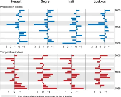
No significant trends in interannual variations in precipitation and streamflow were observed in the four basins over the period 1986–2005. Nevertheless, mean precipita-tion during the first 10 years of the study period was from 4 to 19 % higher than during the last 10 years, except in the Segre basin (−3 %). Furthermore, analysis of the pre-10

cipitation indices (Eq. 1) showed that the wet and dry years in the four basins were the same in nearly half the years (Fig. 2). Mean annual temperature remained almost constant during the 1986–2005 period and the temperature indices (Eq. 2) were the same in the four basins in two thirds of the years (Fig. 2).

IP =(Py−Pey)/σP (1)

15

IT =(Ty−Tey)/σT (2)

where P_y is the annual precipitation for the year y, Pe_y is the median of the annual precipitation,σP is the standard deviation of the annual precipitation.Ty is the annual temperature for the yeary,Te_y is the median of the annual temperature,σ_T is the stan-dard deviation of the annual temperature.

20

3 Models and evaluation procedures

3.1 Statistical downscaling models

(10)

HESSD

12, 10067–10108, 2015

B. Grouillet et al.

Title Page

Tables Figures

◭ ◮

Back Close

Full Screen / Esc

Discussion

P

a

per

|

Discussion

P

a

per

|

Discussion

P

a

per

|

Discussion

P

a

per

|

used climatic patterns on reanalyze grid scale (0.44◦ spatial resolution). These SDMs were thus used to provide the climate data, i.e. precipitation and temperature, used as inputs for the hydrological model at the basin scale. For each variable, three mod-els were calibrated and applied: analogs of atmospheric circulation patterns (ANA), the “cumulative distribution function – transform” approach (CDFt) and a stochastic 5

weather generator (SWG). The analog method and the stochastic weather genera-tor are both calibrated and run on a seasonal basis, using the usual four seasons of the Northern Hemisphere (i.e. DJF, MAM, JJA, SON), whereas the CDFt approach is run on a monthly basis. Sections 3.1.1 to 3.1.3 describe the diff_{erent models and}

Sect. 3.1.4 details the specificity for precipitation modeling. 10

3.1.1 The analog model

The “analogs” model used here is based on the approach of Yiou et al. (2013). For any given day to be downscaled in the validation period, it consists in determining the day in the calibration period with the closest large-scale atmospheric situationXANA. This is determined by minimizing a distance metric (here the Euclidian distance) between 15

the large-scale situation (Xd) of the day to be downscaled and the large-scale situation (Xc) of all the days in the calibration period. More technically, this can be written as:

XANA=argmin(dist(Xd,Xc)) (3)

where argmin(f) is the function returning the minimum value of a functionf, here com-puted over all theXcsituations of the calibration period. Note that this method is applied 20

on the anomalies of the predictors with respect to the seasonal cycle (Yiou et al., 2013). Hereafter this model is referred to as ANA.

3.1.2 The CDFt model

(11)

HESSD

12, 10067–10108, 2015

B. Grouillet et al.

Title Page

Tables Figures

◭ ◮

Back Close

Full Screen / Esc

Discussion

P

a

per

|

Discussion

P

a

per

|

Discussion

P

a

per

|

Discussion

P

a

per

|

to temperature and precipitation, in, for example Vrac et al. (2012) and Vigaud et al. (2013). The CDFt model is a quantile-mapping-based approach, which consists in re-lating the local-scale cumulative distribution function (CDF) of the variable of interest to the large-scale CDF (here from NCEP or GCMs) of the same variable. Let FGc(x) andFOc(x) define the CDFs of the variable of interest, respectively from a GCM (sub-5

script G) and from local-scale observations (subscript O) over the calibration period (subscript c), andF_Gv(x) andF_Ov(x) the CDFs over the validation period (subscript v). First, CDFt estimatesFOv(x) as:

FOv(x)=FOc

F_Gc−1(FGv)

(4)

withx in the range of the physical variable of interest. Then, a quantile-mapping be-10

tweenFGv andFOv is performed to retrieve the physical variable of interest at the local scale. All the technical details on Eq. (4) and subsequent quantile-mapping can be found in Vrac et al. (2012). Note that for this method, only the variable of interest (i.e. precipitation or temperature) at a large scale is used as predictor. It is also worth noting that, when used to downscale GCM values, CDFt does not need to be calibrated with 15

the NCEP reanalyses (unlike ANA and SWG) but is directly calibrated with the GCM data over the calibration period. Indeed, CDFt makes a direct link to bias-correct and downscale the large-scale GCM CDF to the local-scale CDF.

3.1.3 The stochastic weather generator model

The stochastic weather generator (SWG) model used in this study is based on con-20

ditional probability distribution functions in a vector generalized linear model (VGLM) framework, as in Chandler and Wheater (2002). This means that the distribution fam-ily is fixed and the distribution parameters are estimated as functions of the selected predictors. Temperature is expected to follow a Gaussian distribution and rain intensity a Gamma distribution. The meanµand the standard deviationσ of the Gaussian dis-25

(12)

HESSD

12, 10067–10108, 2015

B. Grouillet et al.

Title Page

Tables Figures

◭ ◮

Back Close

Full Screen / Esc

Discussion

P

a

per

|

Discussion

P

a

per

|

Discussion

P

a

per

|

Discussion

P

a

per

|

as functions of the large-scale predictors. The parameters σ, α and β at day i are computed with a common formulation, illustrated here for theα parameter:

log (α_i)=_α0+

N X

j=1

αjX_i,j (5)

with (αj)j=0,···,N the regression coefficients to be estimated,Nthe number of predictors, andX_i,j thejth daily large-scale predictor for dayi. Note that Eq. (5) models the loga-5

rithm of the parameter of interest to ensure that the parameter obtained (σ,α orβ) is positive. The parameterµis formulated in the same way but without the positivity (i.e. log) constraint:

µ_i =_µ0+

N X

j=1

µjX_i_,_j. (6)

As in Vaittinada-Ayar et al. (2015), the predictors used for this model are the two 10

first principal components (PCs) calculated from a principal component analysis (PCA, Barnston and Livezey, 1987) applied separately to each variable.

3.1.4 Modeling rain occurrence

Modeling precipitation is usually divided into two steps: first the occurrence and second the intensity. The modeling of intensity has been introduced in previous sections. The 15

rain occurrence at a given location is modeled as a binomial distributionB(1,p) using a logistic regression (LR, e.g. Buishand et al., 2004; Fealy and Sweeney, 2007). Letpi be the probability of rainfall on dayiconditionally on anNlength predictor (or covariate) vectorX_i=_(X

i1,· · ·,Xi N) as defined in the previous section. The conditional probability of occurrencepi is formulated through a LR as:

(13)

HESSD

12, 10067–10108, 2015

B. Grouillet et al.

Title Page

Tables Figures

◭ ◮

Back Close

Full Screen / Esc

Discussion

P

a

per

|

Discussion

P

a

per

|

Discussion

P

a

per

|

Discussion

P

a

per

|

log _p

i 1−p_i

=_p0+

S=

z }| { N X

j=1

pjX_i,j (7)

p_i = exp(S)

1+_exp(S₎ (8)

where (p0,· · ·,pN) is the vector of coefficients to be estimated. The LR is only used for SWG. The analog and CDFt models directly provide zeros or positive precipitation values.

5

3.2 Hydrological simulations

3.2.1 Hydrological model

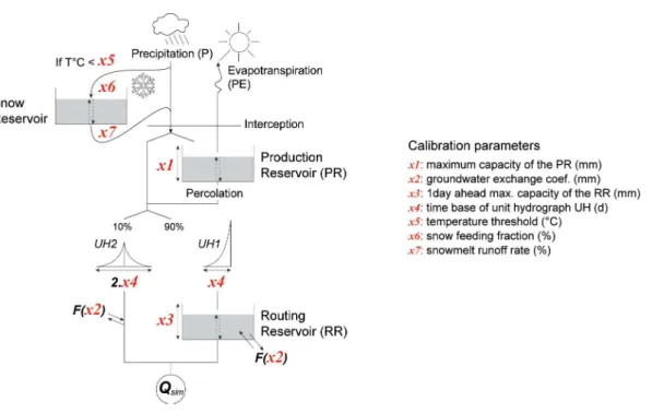
The GR4j lumped conceptual model (Perrin et al., 2003), was chosen to simulate the seasonal and interannual variations in runoff_{at a daily time step (see Fig. 3). Many}

studies have demonstrated the ability of the model to perform well under a wide range 10

of hydro-climatic conditions (e.g. Perrin et al., 2003; Vaze et al., 2010; Coron et al., 2012) and notably in the Mediterranean region (e.g. Tramblay et al., 2013; Fabre et al., 2015; Ruelland et al., 2015). This model relies on precipitation (P) and potential evap-otranspiration (PE) and is based on a production function that determines the eff_ective

precipitation (the fraction of the precipitation involved in runoff_{) that supplies the}

pro-15

duction reservoir and on a routing function based on a unit hydrograph. According to the available data (cf. Sect. 2.2), a simple formula relying on solar radiation and temperature (cf. Eq. 9) was chosen (Oudin et al., 2005) to assess daily potential evap-otranspiration (PE).

PE=Re

λρ× T+₅

100 if (T+5)>0 else PE=0 (9)

(14)

HESSD

12, 10067–10108, 2015

B. Grouillet et al.

Title Page

Tables Figures

◭ ◮

Back Close

Full Screen / Esc

Discussion

P

a

per

|

Discussion

P

a

per

|

Discussion

P

a

per

|

Discussion

P

a

per

|

whereRe is the extraterrestrial solar radiation (MJ m− 2

day−1) given by the Julian day and the latitude,λnet latent heat flux (2.45 MJ kg−1),ρwater density (kg m−3) andT is the mean air temperature at a 2 m height (◦C).

Four parameters are used in the GR4j basic version: the maximum capacity of the soil moisture accounting store x1, a groundwater exchange coeffi_cient_x2_{, the}

maxi-5

mum capacity of routing storagex3, and a time base for unit hydrographsx4. A three-parameter snow module based on catchment-average areal temperature (Ruelland et al., 2011, 2014) was activated to account for the contribution of snow to runoff_from

the catchments. Below a temperature thresholdx5, a fractionx6of precipitation is con-sidered as snowfall; this fraction feeds the snow reservoir. Above the threshold x5, 10

a fractionx7, weighted by the diff_{erence between the daily temperature and the}

thresh-oldx5, is taken from the snow reservoir to represent snowmelt runoff_.

3.2.2 Optimization of hydrological simulations

The model parameters were calibrated and the simulation performances were analyzed by comparing simulated and observed streamflow at a 10 day time step (averaged from 15

daily streamflow outputs) in a multi-objective framework. The following objectives were considered: (i) the overall agreement of the shape of the hydrograph via the Nash– Sutcliff_{e e}ffi_{ciency (NSE) metric (Nash and Sutcli}ff_{e, 1970); (ii) the agreement of the}

low flows via a modified, log version of the NSE criterion; and (iii) the agreement of the runoff_{volume via the cumulated volume error (VE}_C_{) and the mean annual volume error}

20

(VEM).

NSE=₁₋XN

t=1 Q t obs−Q

t sim

2.XN t=1

Qt_obs−Q_sim2

(15)

HESSD

12, 10067–10108, 2015

B. Grouillet et al.

Title Page Abstract Introduction Conclusions References Tables Figures ◭ ◮ ◭ ◮ Back Close

Full Screen / Esc

Printer-friendly Version Interactive Discussion Discussion P a per | Discussion P a per | Discussion P a per | Discussion P a per |

NSElog=1−      PN t=1

logQt_obs+_0.1₋_log_Qt

sim+0.1 2

PN t=1

log Qt_obs+_0.1₋_log_Q_obs

2      (11)

VEC=

XN_years y=1 V

y obs−

XNyears y=1 V

y sim

.XN_years y=1 V

y

obs (12)

VEM=

XNyears y=1

_Vy obs−V

y sim

.V_obsy .Nyears (13)

whereQt_obs and Qt_simare, respectively, the observed and simulated discharges for the 5

time step t,N is the number of time steps for which observations are available, Qy_obs andQ_simy are the observed and simulated volumes for yeary, andNyearsis the number of years in the simulation period.

The NSE criterion is as well-known form of the normalized least squares objective function. Perfect agreement between the observed and simulated values yields an ef-10

ficiency of 1, whilst a negative effi_{ciency represents a lack of agreement worse than if}

the simulated values were replaced with the observed mean values. The optimal value of the VE_C and VE_M criteria is zero. The latter criteria express the relative diff_erence

between observed and simulated values. This multi-objective calibration problem was transformed into a single-objective optimization problem by defining a scalar objective 15

functionFobjthat aggregates the different objective functions:

Fobj=(1−NSE)+(1−NSElog)+|VEC|+VEM. (14)

Calibration was performed in a 7-D parameter space by searching for the minimum value ofFobj. To achieve this high-dimensional optimization efficiently, the shuffle com-plex evolution (SCE) algorithm was used (Duan et al., 1992).

(16)

HESSD

12, 10067–10108, 2015

B. Grouillet et al.

Title Page

Tables Figures

◭ ◮

Back Close

Full Screen / Esc

Discussion

P

a

per

|

Discussion

P

a

per

|

Discussion

P

a

per

|

Discussion

P

a

per

|

3.2.3 Cross-calibration and validation

To test the performance of the hydrological model in contrasted conditions, the calibration-validation periods were sub-divided using a diff_{erential split-sample testing}

(DSST) scheme (Klemeš_{, 1986). Thus, two sub-periods of 10 years each divided}

ac-cording to the median annual precipitation for the period were used either for calibration 5

and for validation.

For the cross calibration-validation process, three calibration-validation periods (for the whole period, for dry years, and for wet years) were used to test the performance of the hydrological model in contrasted conditions. A 2 year warm-up period was included at the beginning of each period to attenuate the eff_{ect of the initialization of storage.}

10

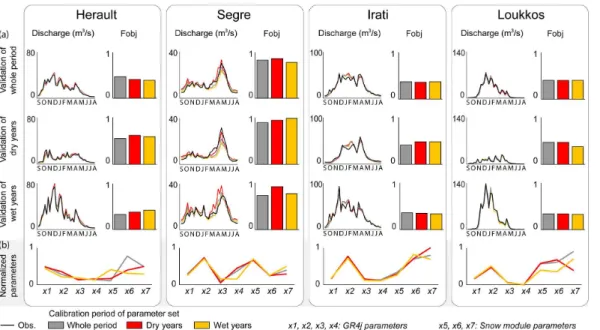
In addition, hydrological years (from September to August) were used in the model-ing process to minimize the boundary limits of the model reservoir. The quality of the simulations was then assessed by comparing the “optimal” parameter set for each cali-bration period. For each basin, three simulations based on the three sets of parameters were compared (see Fig. 4). The four criteria employed for the multi-objective function 15

(NSE, NSE_log, VE_C and VE_M) were used to assess the quality of the simulations.Fobj is optimal at 0, and considered satisfactory below 1.

The hydrographs in Fig. 4a illustrate the ability of the model to correctly simulate runoff_{in the basins, according to the parameter sets used for the calibration periods:}

“whole period”, “dry years” and “wet years”. AllFobj values were below 1, underlining 20

the quality of the simulations. The diff_{erences between the}_F_obj _{of the validation}

simu-lations never exceeded 0.1 (except the Segre basin in the wet year validation period) emphasizing the stability of the simulations under diff_{erent hydro-climatic conditions. In}

the Segre basin, the lower quality of the simulation may be attributed to the very partic-ular hydro-climatic context characterized by a mountainous climatic barrier, which limits 25

(17)

re-HESSD

12, 10067–10108, 2015

B. Grouillet et al.

Title Page

Tables Figures

◭ ◮

Back Close

Full Screen / Esc

Discussion

P

a

per

|

Discussion

P

a

per

|

Discussion

P

a

per

|

Discussion

P

a

per

|

spect to the lower and upper limits of the parameters obtained. As a result, the more the bounds are widened, the less the normalized parameters are able to account for the diff_{erences between the calibration periods. Nonetheless, the relative stability of}

the normalized parameters underlines the robustness of the model under contrasted climatic conditions. However in the Segre basin, diff_{erences on the GR4j native}

param-5

eters reflect the diffi_{culty to correctly simulate runo}ff_{in this basin including NSE values}

of around 0.7. Snow module parameters (x5,x6 and x7) in the Herault and Loukkos basins are less stable but the contribution of snowfall in these basins is rather small. Finally, the low drift of the parameters and the relatively homogeneous quality of the simulations for the whole calibration period, the dry year and wet year calibration peri-10

ods meant we could use the parameter set from the whole period for the downscaled climate-based hydrological simulations. To facilitate interpretation and to limit biases in hydrological modeling when comparing downscaled climate-based hydrological simu-lations, in the following, the whole period hydrological simulation is used as a reference instead of the observation time series.

15

3.3 Comparing downscaling methods from the point of view of water resources

Based on the preliminary calibration of the hydrological model, the quality of runoff

sim-ulations forced by statistically downscaled climate simsim-ulations was evaluated using hy-drological indicators that reflect the main issues of impact studies on water resources. 20

Figure 5 illustrates the diff_{erent steps of this approach.}

First, three low-resolution climate datasets (NCEP, CNRM and IPSL) were down-scaled using three diff_{erent statistical methods (ANALOG, CDFt and SWG) to produce}

new high-resolution hydro-climatic datasets (P andT). Daily PE time series were cal-culated using the same formula (Oudin et al., 2005) as that used to estimate PE from 25

observed temperature.

(18)

hydro-HESSD

12, 10067–10108, 2015

B. Grouillet et al.

Title Page

Tables Figures

◭ ◮

Back Close

Full Screen / Esc

Discussion

P

a

per

|

Discussion

P

a

per

|

Discussion

P

a

per

|

Discussion

P

a

per

|

climatic data (high resolution) and the three raw datasets (low resolution) to produce an ensemble of 12 runoff_{simulations. These simulations were compared to a reference}

runoff_{simulation (REF) corresponding to the model ouputs over the whole reference}

period calibrated with observed climate inputs. This comparison relies on hydrological indicators that are relevant to the water resource challenges according to four comple-5

mentary aspects of the hydrograph: volume of the water flow, interannual and seasonal variability of runoff_{, and streamflow distribution. The water flow volume was assessed}

according to the cumulated volume error (VEC, see Eq. 12). Interannual variability was assessed according to a root mean square error applied to the sorted annual flows. This criterion was then normalized by dividing the RMSE value by the mean of annual 10

observed discharge. Choosing a normalized root mean square error criterion (NRMSE) applied to this distribution gets round the non-synchronicity of the simulations. Note that applying the NRMSE criterion to sorted flows may favor high flows. Seasonal variability was assessed using a NSE criterion (Eq. 10) applied to the mean 10 day discharge series. The last comparison criterion was based on the flow duration profile, divided 15

between high and low flows. High flows correspond to daily flows exceeding the 95th percentile (> Q95), i.e. the 5 % highest daily flows or flows exceeded 5 % of the time. Low flows correspond to daily flows not exceeding the 80th percentile (< Q80), i.e. the 80 % lowest daily flows or flows exceeded 20 % of the time. This value was deliberately chosen to cover a wide range of flows to enable a meaningful distinction between sim-20

ulations while correctly representing low flows. Both high and low flows were evaluated using a NSE criterion applied to the high and low flow time series.

The 12 runoff_{simulations were compared via these five hydrological indicators.}

Fi-nally, the downscaling methods (from the runoff_{simulations forced by the downscaled}

climate time series) were ranked using the same indicators. The median of the related 25

(19)

HESSD

12, 10067–10108, 2015

B. Grouillet et al.

Title Page

Tables Figures

◭ ◮

Back Close

Full Screen / Esc

Discussion

P

a

per

|

Discussion

P

a

per

|

Discussion

P

a

per

|

Discussion

P

a

per

|

datasets to make it possible to rank them. Finally, an additional criterion (Eq. 15) was used to aggregate the diff_{erent goodness-of-fit criteria to provide an overview of the}

performance of the diff_{erent downscaling models driven by distinct climate datasets.}

The lower the aggregation criterion, the better the ranking.

IAGG=|VEC|+NRMSEINT+(1−NSESEAS)+(1−NSEHF)+(1−NSELF) (15) 5

For the remainder of this paper, REF refers to the runoff _{simulation with the best}

set of parameters obtained by calibration over the whole period and forced by the high-resolution observed climate data: RAW refers to the simulations with raw low-high-resolution climate data from NCEP/NCAR reanalysis or GCMs outputs over the reference period. ANA, CDFt and SWG refer to the simulations with downscaled climate data respectively 10

via ANALOG, CDFt and SWG methods.

4 Comparative analysis of hydrological responses to downscaled climate forcings

4.1 General principles of the comparative analysis

Before performing the sensitivity analysis per indicator, the climate data sets and the 15

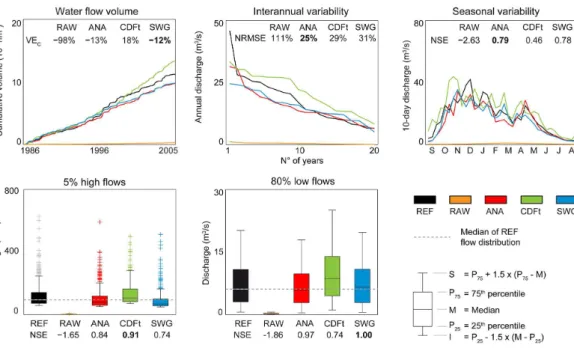
downscaling methods were analyzed and compared individually for each basin. The comparison is presented according to NCEP/NCAR reanalysis, with CNRM and IPSL data as inputs in the downscaling models. Figure 6 shows the use of a dashboard to compare the downscaling methods in a single basin, which summarizes the results obtained from NCEP-based large- or local-scale simulations in the Herault basin. 20

First, this example shows that the quality of simulated flows depends to a great extent on the downscaling method. RAW-based simulations confirm the benefits of downscaling climate data to reproduce diff_{erent aspects of the reference hydrograph.}

Second, the downscaling methods will be ranked diff_{erently depending on the indicator}

(20)

HESSD

12, 10067–10108, 2015

B. Grouillet et al.

Title Page

Tables Figures

◭ ◮

Back Close

Full Screen / Esc

Discussion

P

a

per

|

Discussion

P

a

per

|

Discussion

P

a

per

|

Discussion

P

a

per

|

For example, in the Herault basin with NCEP-based simulations, the ANALOG method reproduces the mean seasonal variability of runoff_{better than the other methods, with}

NSE values of 0.79. In contrast, the SWG method reproduces the interannual variability and water flow volume better, and although the CDFt method reproduces high flows better, it reproduces low flows less well than the other models.

5

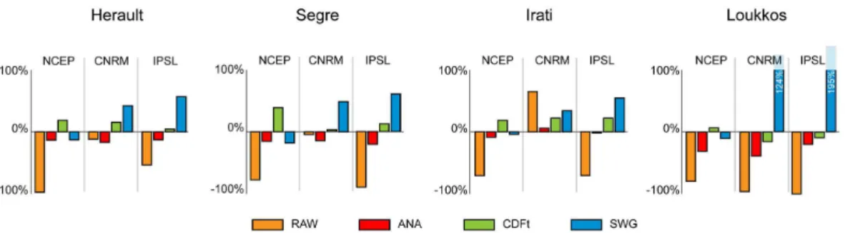
4.2 Water volumes

Water volumes were assessed through the cumulative volume error, i.e. the error in the percentage of the cumulated volume of water flow over the whole period. ANALOG-based simulations generally reproduced water volumes better than the other simula-tions. Nevertheless, diff_{erences appeared depending on the input data used (NCEP,}

10

CNRM or IPSL) and on the basin concerned (Fig. 7). Except in the Loukkos basin and for CNRM in the Herault and Segre basin, RAW-based simulations were always improved by downscaling. CDFt-based simulations were slightly better than ANALOG-based simulations in reproducing cumulated volume of water with VE_Cabsolute values averaged between the four basins, with 12 % for CDFt and with 14 % for ANALOG. In 15

addition, the results of ANALOG-based simulations were more constant without out-lier criterion values. Criterion values are considered as outout-liers when VE_C is greater than 50 %. In the Loukkos basin, simulations provided many outliers with both SWG and CDFt. The CDFt method improved the results according to the VECcriterion better than the other models. SWG-based simulations ranked first for both criteria with NCEP 20

as inputs, but performed poorly with GCMs.

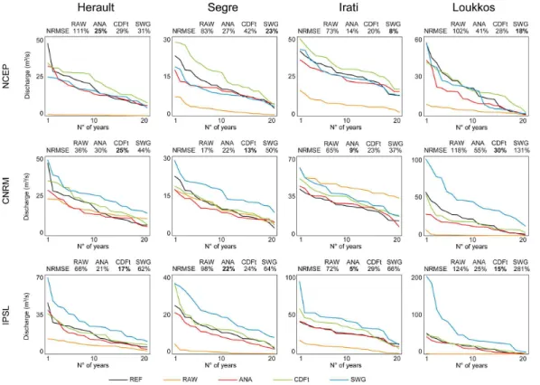
4.3 Interannual variability of streamflow

The ability to reproduce interannual runoff_{variability was assessed through a root mean}

square error (NRMSE_INT) criterion applied to the sorted time series of annual discharge and normalized by dividing RMSE by the mean annual discharge of the reference (see 25

(21)

HESSD

12, 10067–10108, 2015

B. Grouillet et al.

Title Page

Tables Figures

◭ ◮

Back Close

Full Screen / Esc

Discussion

P

a

per

|

Discussion

P

a

per

|

Discussion

P

a

per

|

Discussion

P

a

per

|

the annual discharge values were sorted from the highest value to the lowest one to generate new decreasing time series on which the NRMSE criterion was calculated with respect to the sorted reference time series. The results show that the interannual variability of runoff _{is correctly reproduced by the simulations based on most of the}

downscaled climate datasets, particularly ANALOG- and CDFt-based simulations in 5

which NRMSE values rarely reached more than 30 %. On the whole, RAW-based sim-ulations were improved by downscaling, especially when driven by NCEP and IPSL, except for SWG-based simulations driven by GCMs (Fig. 8). Indeed, when driven by NCEP, the SWG method reproduced interannual variability better than the other meth-ods for three of the four basins, but produced poor results with GCMs, in which case 10

ANALOG- and CDFt-based simulations generally performed better.

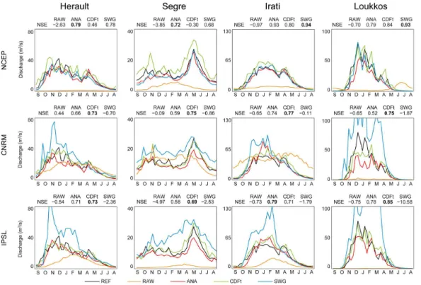
4.4 Seasonal variability of streamflow

Seasonal variability was assessed using an NSE criterion (Eq. 10) applied to the mean 10 day discharge series. In most cases, the downscaling methods improved the repro-duction of the seasonal variability of streamflow compared to the low-resolution raw 15

datasets (see Fig. 9). This was particularly true of NCEP reanalyses, for which down-scaled inputs considerably improved the simulation of the seasonal dynamics more realistically than with RAW-based simulations. Although the ANALOG method did not systematically match the best NSE values, on the whole, the method reproduced the seasonal variability better than CDF-t and SWG. The CDFt method performed par-20

ticularly well with GCMs as inputs, but proved to be unsuitable with NCEP under the particular hydro-climatic conditions that prevail in the Segre basin. Except with NCEP, SWG-based simulations reproduced seasonal variability poorly, more in terms of inten-sity than occurrence: as a result, with this SDM, the shape of the streamflow season-ality was reasonably well reproduced but not the values of discharge.

(22)

HESSD

12, 10067–10108, 2015

B. Grouillet et al.

Title Page

Tables Figures

◭ ◮

Back Close

Full Screen / Esc

Discussion

P

a

per

|

Discussion

P

a

per

|

Discussion

P

a

per

|

Discussion

P

a

per

|

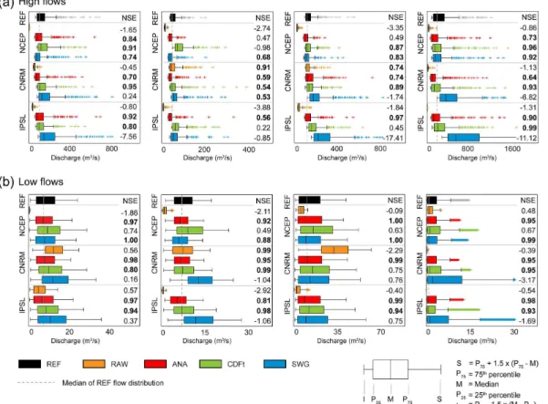
4.5 Streamflow distribution: high and low flows

Streamflow distribution was divided between high flows, i.e. the 5 % highest daily flows, and low flows, i.e. the 80 % lowest daily flows. Both were evaluated using a NSE cri-terion applied to the high and low flow time series. On the whole, the downscaling methods improved the reproduction of the distribution of sorted high flows (Fig. 10a). 5

However, it should be noted that the downscaled simulations with CNRM data deterio-rated raw data in the Segre basin. Due to the nature of the “high flows” indicator and the NSE criterion used to evaluate it, the reproduction of high flows was considered to be satisfactory for NSE values greater than 0.5. Results showed that ANALOG generally reproduced the 5 % highest flows best; the NSE values were quite stable and never 10

below 0.47. The CDFt-based simulation results were very close to those obtained with ANALOG, with equivalent scores when NCEP or GCM data were used as inputs. Nev-ertheless, CDFt appeared to be less able to reproduce high flows in the Segre basin characterized by a hydrological context including snowmelt. The SWG method repro-duced high flows well with NCEP data as inputs, but not with GCM data.

15

Figure 10b shows the distribution of sorted low flows and the associated NSE crite-rion. The reproduction of low flows was considered to be satisfactory when NSE val-ues were higher than 0.8. Moreover, applying a NSE criterion to the sorted low flows tended to emphasize the diff_{erences between the simulations and thus made it easy}

to distinguish simulations that reproduced low flows poorly. The downscaling methods 20

improved the representation of the 80 % lowest flows in all basins, except for the SWG method with GCM data used as inputs. In general, the best results were obtained from ANALOG-based simulations, with NSE values always above 0.81. The CDFt-based simulations performed significantly better when forced with GCMs than with NCEP. The SWG-based simulations were unable to reproduce low flows when GCMs data 25

(23)

HESSD

12, 10067–10108, 2015

B. Grouillet et al.

Title Page

Tables Figures

◭ ◮

Back Close

Full Screen / Esc

Discussion

P

a

per

|

Discussion

P

a

per

|

Discussion

P

a

per

|

Discussion

P

a

per

|

5 Discussion and conclusions

The aim of this study was to test the ability of diff_{erent statistical downscaling climate}

models to provide accurate hydrological simulations for use in climate change impact studies (CCIS) on water resources. To get round the constraints represented by the inherent characteristics of each climate model, we compared three statistical down-5

scaling methods applied on three low resolution raw datasets: NCEP/NCAR reanalysis data and two GCM data (CNRM and IPSL). The three downscaling methods were an analog method (ANALOG), a stochastic weather generator (SWG) and the “cumula-tive distribution function – transform” approach (CDFt). This allowed us to analyze the sensitivity of runoff _{modeling at the catchment scale to 12 climatic series (three raw}

10

low-resolution datasets and nine downscaled high-resolution datasets). The sensitivity analysis was based on a previously calibrated hydrological model validated with local hydro-climatic observed data over a 20 year reference period. The model simulations served as a benchmark for the comparison between the raw and downscaled datasets from NCEP reanalysis and GCM outputs over the same period. The comparison with 15

the runoff _{simulations forced with raw and downscaled climate datasets was based}

on hydrological indicators describing the main features of the hydrograph: the ability to reproduce the cumulated volume of water flow, interannual and seasonal variability of runoff_{, and the distribution of streamflow events, including high and low flows. To}

account for uncertainty related to the spatial variability of the downscaled climate sim-20

ulations, this approach was applied over four western Mediterranean basins of similar size but that represent a with a wide range of hydro-meteorological situations.

The proposed sensitivity analysis enabled us to identify the strengths and weak-nesses of diff_{erent statistical downscaling methods with respect to the sensitivity of}

runoff_{simulations to low-resolution and high-resolution downscaled climate datasets}

25

(24)

cli-HESSD

12, 10067–10108, 2015

B. Grouillet et al.

Title Page

Tables Figures

◭ ◮

Back Close

Full Screen / Esc

Discussion

P

a

per

|

Discussion

P

a

per

|

Discussion

P

a

per

|

Discussion

P

a

per

|

matologists for assessing the suitability of SDMs based on predictors and reanalyze grids (see e.g. Vaittinada-Ayar et al., 2015), we focused on a validation protocol directly based on streamflow thus allowing the combined impacts of the downscaled precipita-tion and temperature inputs to be considered through the hydrological response.

On the whole, the ANALOG-based simulations performed well in all the situations 5

tested, whatever the large-scale climate dataset used as inputs (NCEP or GCMs), no-tably in reproducing interannual and seasonal runoff _{and low flows. ANALOG-based}

simulations were closely followed by CDFt-based simulations, notably when GCM out-puts were used, but with a lower variability of scores than with ANALOG. To the con-trary, the results clearly showed that the SWG method should not be used “as is” in 10

climate change impact studies on water resources. Indeed, although the SWG-based simulations were satisfactory when based on the NCEP large-scale climate dataset, they significantly underperformed when based on GCM outputs. Biases of the GCM data with respect to the NCEP/NCAR reanalyses may explain the poor performances of the SWG method. As SWG is calibrated with “perfect” predictors from reanalyses, 15

its application to biased GCM predictors led to unsatisfactory SWG-based hydrologi-cal simulations. To make the SWG method more applicable in climate change impact studies on runoff_{, one solution could be correcting the GCMs predictors with respect to}

reanalyses, as done for example by Colette et al. (2012) before performing a dynamical downscaling.

20

lthough the ANALOG method appeared to be the best SDM in this study, it may suff_er

from certain limitations when used in a climate change context, notably when down-scaling GCM projections over the 21st century. One main limitation is that ANALOG is not able to provide suitable simulations for the extreme events if such events increase in intensity in the future (see e.g. Teng et al., 2012). Indeed, by construction, as ANALOG 25

works by resampling the calibration set, it never supplies downscaled values beyond the range of the calibration reference dataset.

(25)

HESSD

12, 10067–10108, 2015

B. Grouillet et al.

Title Page

Tables Figures

◭ ◮

Back Close

Full Screen / Esc

Discussion

P

a

per

|

Discussion

P

a

per

|

Discussion

P

a

per

|

Discussion

P

a

per

|

the chosen indicators. The CDFt method was particularly appropriate when we focused on the cumulated volume, seasonal variability and high flows. In addition, it should be noted that the CDFt method is the most parsimonious technique since it generally needs only one variable as predictor. This could obviously be considered an advan-tage since the complexity of CDFt is very low. However, this low level of complexity 5

could mean that some climate information needed to drive the CDFt more effi_ciently

will be missing. In that sense, one possible improvement could consist in incorporating additional covariates in CDFt, as done by Kallache et al. (2011). Nevertheless, the ap-proach including those additional predictors means that this conditional CDFt has to be calibrated on reanalyses or, at a minimum, on the outputs of a climate model of which 10

the day-to-day evolution of large-scale weather states matches that of the real world. This could be a limitation, since additional biases may appear with those constraints.

The next step will be exploring the potential impact of climate change on the runoff

in the basins studied here. To this end, an ensemble approach will be proposed based on the construction of high-resolution climate scenarios using diff_{erent climate models,}

15

gas emission scenarios, and downscaling techniques. In view of the acceptable hy-drological simulations obtained with ANALOG and CDFt methods, it may be useful to develop high-resolution climate forcings downscaled with these two methods in order to account for the uncertainty of the downscaling, as recommended by some authors (e.g. Chen et al., 2011, 2012) for applications in climate change impact studies. Our study 20

also showed the benefits of evaluating the relevance of SDMs in a given hydro-climatic context using a suitable validation protocol. Indeed, selecting unsuitable downscaling methods, such as SWG with GCM outputs, can expand the range of uncertainty linked to the range of SDMs.

Although it is commonly acknowledged that the uncertainty resulting from climate 25

(26)

HESSD

12, 10067–10108, 2015

B. Grouillet et al.

Title Page

Tables Figures

◭ ◮

Back Close

Full Screen / Esc

Discussion

P

a

per

|

Discussion

P

a

per

|

Discussion

P

a

per

|

Discussion

P

a

per

|

et al., 2015; Ruelland et al., 2015) showed that the choice of the hydrological model (structural uncertainty) and its parameterization (parameter uncertainty) could cause significant variability in runoff_{simulations. Consequently, further analyses of the}

appli-cability of the model parameters in a non-stationary context and with diff_erent

calibra-tion criteria are needed before the model is used in future climate condicalibra-tions. 5

Similarly, the diff_{erent sources of uncertainties and their propagation in the}

hydrologi-cal projections need to be evaluated. To this end, a standard ensemble approach based on various climatic, downscaling and hydrological models may not be suffi_{cient, since}

using many models without prior validation of their effi_{ciency can lead to very large}

uncertainty bounds due to the poor quality of some models in the ensemble frame-10

work. Minimizing uncertainty thus requires selecting models that perform reasonably well over the reference period in the context of current climate. Although this cannot guarantee the quality of the models for future conditions, we believe it is an essential step to provide more reliable and relevant hydrological projections.

Acknowledgements. This work was part of the StaRMIP project (Statistical Regionalization

15

Models Inter-comparisons and hydrological impacts Project, grant agreement ANR-12-JS06-0005-01), and the REMEMBER project (grant agreement ANR-12-SENV-0001-01), both funded by the French National Research Agency (ANR), as well as part of the GICC REMedHE project (2012–2015) funded by the French Ministry of Ecology, Sustainable Development and Energy and the ENVI-MedCLIHMag(Changement cLimatique et Impacts Hydrologiques au Maghreb) 20

project funded by the program INSU-MISTRALS.

References

Arnell, N. W.: Uncertainty in the relationship between climate forcing and hydrological response in UK catchments, Hydrol. Earth Syst. Sci., 15, 897–912, doi:10.5194/hess-15-897-2011, 2011. 10091

25

(27)

HESSD

12, 10067–10108, 2015

B. Grouillet et al.

Title Page

Tables Figures

◭ ◮

Back Close

Full Screen / Esc

Discussion

P

a

per

|

Discussion

P

a

per

|

Discussion

P

a

per

|

Discussion

P

a

per

|

Benke, K. K., Lowell, K. E., and Hamilton, A. J.: Parameter uncertainty, sensitivity analysis and prediction error in a water-balance hydrological model, Math. Comput. Model., 47, 1134– 1149, 2008. 10091

Brigode, P., Oudin, L., and Perrin, C.: Hydrological model parameter instability: a source of additional uncertainty in estimating the hydrological impacts of climate change?, J. Hydrol., 5

476, 410–425, 2013. 10091

Buishand, T. A., Shabalova, M. V., and Brandsma, T.: On the choice of the temporal aggregation level for statistical downscaling of precipitation, J. Climate, 17, 1816–1827, 2004. 10078 Chandler, R. E. and Wheater, H. S.: Analysis of rainfall variability using generalized

lin-ear models: a case study from the west of Ireland, Water Resour. Res., 38, 1192, 10

doi:10.1029/2001WR000906, 2002. 10077

Chen, H., Xu, C. Y., and Guo, S.: Comparison and evaluation of multiple GCMs, statistical downscaling and hydrological models in the study of climate change impacts on runoff_{, J.}

Hydrol., 434–435, 36–45, 2012. 10070, 10091

Chen, J., Brissette, F. P., and Leconte, R.: Uncertainty of downscaling method in quantifying 15

the impact of climate change on hydrology, J. Hydrol., 401, 190–202, 2011. 10070, 10091 Colette, A., Vautard, R., and Vrac, M.: Regional climate downscaling with prior

sta-tistical correction of the global climate forcing, Geophys. Res. Lett., 39, l13707, doi:10.1029/2012GL052258, 2012. 10090

Coron, L., Andréassian, V., Perrin, C., Lerat, J., Vaze, J., Bourqui, M., and Hendrickx, F.: Crash 20

testing hydrological models in contrasted climate conditions: an experiment on 216 Australian catchments, Water Resour. Res., 48, w05552, doi:10.1029/2011WR011721, 2012. 10079 Dezetter, A., Fabre, J., Ruelland, D., and Servat, E.: Selecting an optimal climatic dataset for

in-tegrated modeling of the Ebro hydrosystem, in: Hydrology in a Changing World: Environmen-tal and Human Dimensions, Proc. 7th FRIEND Int. Conf., 7–10 October 2014, Montpellier, 25

France, IAHS-AISH P., 363, 355–360, 2014. 10073

Diaz-Nieto, J. and Wilby, R. L.: A comparison statistical downscaling and climate change factor methods: impacts on low flows in the river Thanes, United Kingdom, Climatic Change, 69, 245–268, 2005. 10070

Dibike, Y. B. and Coulibaly, P.: Hydrologic impact of climate change in the Saguenay watershed: 30