UNIVERSIDADE NOVA DE LISBOA
Faculdade de Ciências e Tecnologia
Departamento de Ciências e Engenharia do Ambiente
ASSESSMENT OF CLIMATE CHANGE STATISTICAL DOWNSCALING
METHODS
Application and comparison of two statistical methods to a single site in Lisbon
Pedro Miguel de Almeida Garrett Graça Lopes
Dissertação apresentada na Faculdade de Ciências e Tecnologia
da Universidade Nova de Lisboa para a obtenção do grau de
Mestre em Engenharia do Ambiente.
Dissertação realizada sob a orientação de:
Profª Doutora Maria Júlia Fonseca de Seixas
ACKNOWLEDGMENTS
ABSTRACT_______________________________________________
Climate change impacts are very dependent on regional geographical features, local climate variability, and socio-economic conditions. Impact assessment studies on climate change should therefore be performed at the local or at most at the regional level for the evaluation of possible consequences. However, climate scenarios are produced by Global Circulation Models for the entire Globe with spatial resolutions of several hundred kilometres. For this reason, downscaling methods are needed to bridge the gap between the large scale climate scenarios and the fine scale where local impacts happen.
An overview on downscaling techniques is presented, referring the main limitation and advantages on dynamical, statistical and statistical-dynamic approaches. For teams with limited computing power and non-climate experts, statistical downscaling is currently the most feasible approach at obtaining climate data for future impact studies.
To assess the capability of statistical downscaling methods to represent local climate variability it is shown an inter-comparison and uncertainties analysis study between a stochastic weather generator, using LARS-WG tool, and a hybrid of stochastic weather generator and transfer function methods, using the SDSM tool. Models errors and uncertainties were estimated using non-parametric statistical methods at the 95% confidence interval for precipitation, maximum temperature and minimum temperature for the mean and variance for a single site in Lisbon.
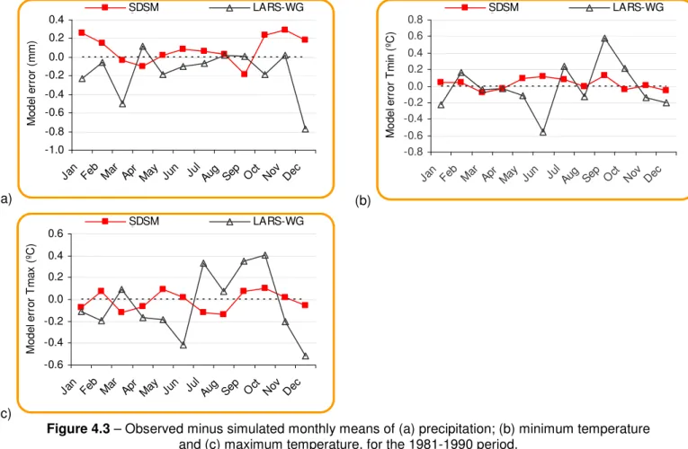
The comparison between the observed dataset and the simulations showed that both models performance are acceptable. However, the SDSM tool was able to better represent the minimum and maximum temperature while LARS-WG simulations on precipitation are better. The analysis of both models uncertainties for the mean are very close to the observed data in all months, but the uncertainties for the variances showed that the LAR-WG simulation performance is slightly better for precipitation and that both model simulations for minimum and maximum temperature are very close from the observed.
RESUMO______________________________________________
Os impactes das alterações climáticas estão estritamente dependentes das características geográficas, variabilidade climática local e das condições sócio-económicas. Desta forma, a avaliação de impactes deverá ser feita à escala local ou pelo menos a uma escala regional. No entanto, cenários futuros de alterações climáticas são produzidos por Modelos de Circulação Global para todo o planeta com resoluções espaciais de várias centenas de quilómetros, dificultando a tarefa de avaliação dos seus efeitos localmente. Para fazer a ponte entre a escala global e local existem métodos matemáticos de “downscaling” que permitem produzir simulações de dados climáticos futuros.
Este trabalho apresenta uma revisão de várias técnicas de “downscaling” abordando as limitações e vantagens de métodos dinâmicos, estatísticos e estatistico-dinâmicos, focando com mais detalhe os métodos estatísticos por serem acessíveis a não peritos em climatologia e exigirem poucos recursos computacionais.
Foi desenvolvido um estudo comparativo entre um gerador de clima, usando a ferramenta LARS-WG, e um método híbrido entre gerador de clima e de equações de transferência usando a ferramenta SDSM. A avaliação de erros e de incertezas foram calculadas usando métodos estatísticos não-paramétricos para avaliar a média e a variância, para um intervalo de confiança de 95% para a precipitação, temperatura máxima e temperatura mínima para um único local em Lisboa.
A comparação entre as simulações e os dados observados demonstram que ambos os métodos têm uma boa e semelhante performance. No entanto, a ferramenta SDSM consegue simular melhor a temperatura máxima e mínima, enquanto que o gerador de clima apresenta um melhor desempenho a simular a precipitação. No que diz respeito à avaliação de incertezas em torno da média, ambos os métodos apresentam resultados muito semelhantes aos observados. No entanto, as incertezas associadas à variância da precipitação foram melhor representadas pelo gerador de clima, mas ambos os métodos apresentam resultados semelhantes aos observados para a variância da temperatura mínima e máxima.
GLOSSARY_______________________________________________
The following definitions were drawn from the Glossary of terms in the Summary for Policymakers, a Report of Working Group I of the Intergovernmental Panel on Climate Change, and the Technical Summary of the Working Group I Report.
Atmosphere - The gaseous envelope surrounding the Earth, comprising almost entirely of
nitrogen (78.1%) and oxygen (20.9%), together with several trace gases, such as argon (0.93%) and greenhouse gases such as carbon dioxide (0.03%).
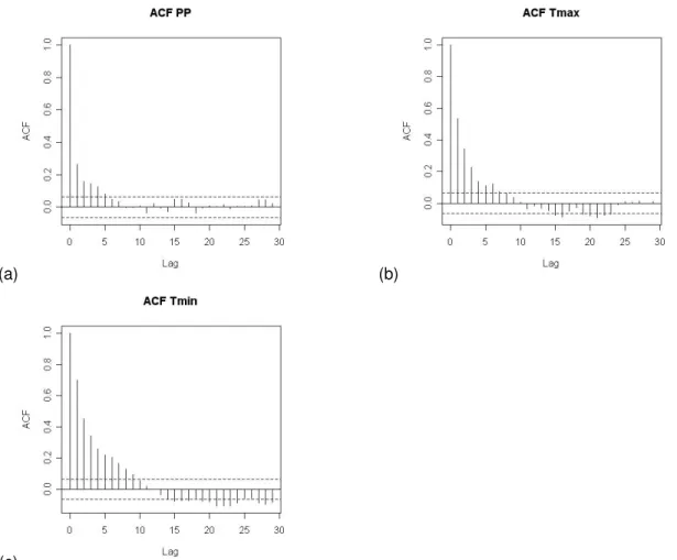
Autocorrelation - A measure of the linear association between two separate values of the
same random variable. The values may be separated in either space or time. For time series, the autocorrelation measures the strength of association between events separated by a fixed interval or lag. The autocorrelation coefficient varies between –1 and +1, with unrelated instances having a value of zero. For example, temperatures on successive days tend to be positively autocorrelated.
Climate - The “average weather” described in terms of the mean and variability of relevant
quantities over a period of time ranging from months to thousands or millions of years. The classical period is 30 years, as defined by the World Meteorological Organisation (WMO).
Climate change - Statistically significant variation in either the mean state of the climate, or in its variability, persisting for an extended period (typically decades or longer). Climate change may be due to natural internal processes or to external forcings, or to persistent anthropogenic changes in the composition of the atmosphere or in land use.
Climate model - A numerical representation of the climate system based on the physical,
chemical and biological properties of its components, their interactions and feedback processes, and accounting for all or some its known properties.
Climate prediction - An attempt to produce a most likely description or estimate of the
actual evolution of the climate in the future, e.g. at seasonal, inter–annual or long– term time scales.
Climate projection - A projection of the response of the climate system to emission or
Climate scenario - A plausible and often simplified representation of the future climate,
based on an internally consistent set of climatological relationships, that has been constructed for explicit use in investigating the potential consequences of anthropogenic climate change.
Climate variability - Variations in the mean state and other statistics (such as standard
deviations, the occurrence of extremes, etc.) of the climate on all temporal and spatial scales beyond that of individual weather events.
Conditional process - A mechanism in which an intermediate state variable governs the
relationship between regional forcing and local weather. For example, local precipitation amounts are conditional on wet–day occurrence (the state variable), which in turn depends on regional–scale predictors such as atmospheric humidity and pressure.
Deterministic - A process, physical law or model that returns the same predictable outcome
from repeat experiments when presented with the same initial and boundary conditions, in contrast to stochastic processes.
Domain - A fixed region of the Earth’s surface and over-lying atmosphere represented by a
Regional Climate Model. Also, denotes the grid box(es) used for statistical downscaling. In both cases, the downscaling is accomplished using pressure, wind, temperature or vapour information supplied by a host GCM.
Downscaling - The development of climate data for a point or small area from regional
climate information. The regional climate data may originate either from a climate model or from observations. Downscaling models may relate processes operating across different time and/or space scales.
Emission scenario - A plausible representation of the future development of emissions of
substances that are potentially radiatively active (e.g. greenhouse gases, aerosols), based on a coherent and internally consistent set of assumptions about driving forces and their key relationships.
Extreme weather event - An event that is rare within its statistical reference distribution at a
particular place. Definitions of “rare” vary from place to place (and from time to time), but an extreme event would normally be as rare or rarer than the 10th or 90th percentile.
General Circulation Model (GCM) - A three–dimensional representation of the Earth’s
thermodynamics) and momentum (Newton’s second law of motion), along with the conservation of mass (continuity equation) and water vapour (ideal gas law). Each equation is solved at discrete points on the Earth’s surface at fixed time intervals (typically 10–30 minutes), for several layers in the atmosphere defined by a regular grid (of about 200km resolution). Couple ocean–atmosphere general circulation models (O/AGCMs) also include ocean, land–surface and sea–ice components. See climate model.
Grid - The co–ordinate system employed by GCM or RCM to compute three– dimensional fields of atmospheric mass, energy flux, momentum and water vapour. The grid spacing determines the smallest features that can be realistically resolved by the model. Typical resolutions for GCMs are 200km, and for RCMs 20–50km.
NCEP - The acronym for the National Center for Environmental Prediction. The source of
re–analysis (climate model assimilated) data widely used for dynamical and statistical downscaling of the present climate.
Predictand - A variable that may be inferred through knowledge of the behaviour of one or
more predictor variables.
Predictor - A variable that is assumed to have predictive skill for another variable of interest,
the predictand. For example, day–to–day variations in atmospheric pressure may be a useful predictor of daily rainfall occurrence.
Probability Density Function (PDF) - A distribution describing the probability of an
outcome for a given value for a variable. For example, the PDF of daily temperatures often approximates a normal distribution about the mean, with small probabilities for very high or low temperatures.
Re–gridding A statistical technique used to project one co–ordinate system onto
another, and typically involving the interpolation of climate variables. A necessary
pre–requisite to most statistical downscaling, because observed and climate model
data are seldom archived using the same grid system.
Regional Climate Model (RCM) - A three–dimensional, mathematical model that simulates
Regression - A statistical technique for constructing empirical relationships between a
dependent (predictand) and set of independent (predictor) variables. See also black box,
transfer function.
Relative humidity - A relative measure of the amount of moisture in the air to the amount
needed to saturate the air at the same temperature expressed as a percentage.
Resolution - The grid separation of a climate model determining the smallest physical feature that can be realistically simulated.
Scenario - A plausible and often simplified description of how the future may develop based
on a coherent and internally consistent set of assumptions about driving forces and key relationships. Scenarios may be derived from projections, but are often based on additional information from other sources, sometimes combined with a “narrative story–line”.
Stochastic - A process or model that returns different outcomes from repeat experiments
even when presented with the same initial and boundary conditions, in contrast to
deterministic processes. See weather generator.
Transfer function - A mathematical equation that relates a predictor, or set of predictor variables, to a target variable, the predictand. The predictor(s) and predictand represent processes operating at different temporal and/or spatial scales. In this case, the transfer function provides a means of downscaling information from coarse to finer resolutions.
Uncertainty - An expression of the degree to which a value (e.g. the future state of the
climate system) is unknown. Uncertainty can result from a lack of information or from disagreement about what is known or knowable. It can also arise from poorly resolved climate model parameters or boundary conditions.
Unconditional process - A mechanism involving direct physical or statistical link(s)
between a set of predictors and the predictand. For example, local wind speeds may be a function of regional airflow strength and vorticity.
Weather generator - A model whose stochastic (random) behaviour statistically resembles
Weather pattern - An objectively or subjectively classified distribution of surface (and/or
INDEX_OF CONTENTS______________________________________
1 INTRODUCTION ... 1
1.1
Global Climate Models and scenarios ... 1
1.2
Downscaling climate change data... 3
2 OVERVIEW ON CLIMATE DOWNSCALING APPROACHES ... 7
2.1
Dynamical Downscaling ... 8
2.2
Statistical Downscaling... 10
2.3
Statistical-dynamical downscaling... 13
3 IMPLEMENTATION OF STATISTICAL DOWNSCALING METHODS TO A SINGLE SITE IN LISBON ... 15
3.1
Case study description ... 15
3.2
Baseline meteorological data ... 17
3.3
Climatic data for future scenarios ... 18
3.4
LARS-WG: a stochastic weather generator ... 18
3.4.1
Site Analysis ... 19
3.4.2
Model validation ... 20
3.4.3
Creating climate change scenarios... 20
3.5
SDSM: a multi-regression model... 21
3.5.1
Quality control and data transformation ... 21
3.5.2
Screening of downscaling predictor variables ... 21
3.5.3
Model calibration and selection ... 22
3.5.4
Model validation ... 25
3.5.5
Scenario generation from GCM predictors... 25
4 MODEL VALIDATION AND UNCERTAINTY ANALYSIS OF LARS-WG AND SDSM SIMULATIONS FOR THE CASE STUDY... 27
4.1
Exploratory analysis... 27
4.2
Assessment of errors of the estimates of means and variances ... 30
4.2.1
Evaluation of the errors in the estimates of means ... 30
4.2.2
Evaluation of the errors in the estimates of variances ... 32
4.3
Confidence intervals of the estimates of means and variances... 34
4.3.1
Uncertainties in the estimates of means... 34
4.3.2
Uncertainties in the estimates of variance ... 35
4.4
Additional analysis: Skewness and Wet-spell length of precipitation data ... 37
5 2041-2070 SDSM AND LARS-WG RESULTS FOR THE A2A SRES SCENARIO... 39
5.1
Summary statistics for Lisbon using LARS-WG for the A2a SRES scenario ... 39
5.2
Summary statistics for a single site in Lisbon using SDSM for the A2a SRES
scenario ... 41
6 CONCLUSION AND FUTURE WORK ... 45
6.1
Dynamical and statistical downscaling... 45
6.2
Comparison of two statistical downscaling methods: LARS-WG / SDSM ... 46
INDEX_OF TABLES_________________________________________
Table 3.1 – Relative change (SCENARIO/BASELINE) between the GCM future scenario (2041-2070) and GCM baseline period using the daily dataset... 20
Table 3.2 – List of predictors chosen for each climate variable... 22 Table 3.3 – Coefficient of determination R2 and Durbin-Watson statistics for validating the
independence assumption for the maximum temperature model. ... 23
Table 3.4 – Coefficient of determination R2 and Durbin-Watson statistics for validating the
independence assumption for the minimum temperature model. ... 24 Table 3.5 – Coefficient of determination R2 and Durbin-Watson statistics for validating the
independence assumption for the precipitation model. [n.a. = not available] ... 24
Table 4.1 – Test results (p values) of the Mann-Whitney U test for the difference of means of the observed (1981-1990) and downscaled daily Tmin, Tmax and precipitation for each month at the 95% confidence level. ... 32
Table 4.2 – Test results (p values) of the Brown-Forsythe test for the difference of variances of the observed and downscaled daily Tmin, Tmax and precipitation for each month at the 95% confidence level. ... 34
INDEX_OF FIGURES______________________________________
Figure 2.1 – Main steps in obtaining and using downscaled climate scenarios by way of statistical approaches. ... 7
Figure 3.1 – GCM HadCM3 global grid (96x73); each point represents the centre of the grid box. ... 16 Figure 3.2 – Web based tool to extract global climate data to one chosen grid box... 19 Figure 3.3 - Histogram of the residuals to check normality for the maximum temperature model. ... 23 Figure 3.4 – Residuals vs predicted value to check homogeneity for the maximum temperature model. ... 23
Figure 3.5 – Histogram of the residuals to check normality for the minimum temperature model. ... 24 Figure 3.6 – Residuals vs predicted value to check homogeneity for the minimum temperature model.
... 24
Figure 3.7 – Histogram of the residuals to check normality for the precipitation model... 24 Figure 3.8– Residuals vs predicted value to check homogeneity for the precipitation model... 24 Figure 4.1– Exploratory data analysis of (a) daily precipitation (PP); (b) daily maximum temperature (Tmax); (c) daily minimum temperature (Tmin) for January (1961-1990) at the “Lisboa Geofísica” station. ... 28
Figure 4.2 – ACF plots of (a) daily precipitation; (b) daily maximum temperature and (c) daily
minimum temperature for January (1961-1990) at the “Lisboa Geofísica” station... 29
Figure 4.3 – Observed minus simulated monthly means of (a) precipitation; (b) minimum temperature and (c) maximum temperature, for the 1981-1990 period... 31
Figure 4.4– Estimation of the monthly average of daily observed and simulated variances for (a) precipitation; (b) maximum temperature and (c) minimum temperature for the 1981-1990 time period.
Figure 4.5 – 97.5 percentile for the mean using a non-parametric bootstrap approach for (a) daily precipitation; (b) daily minimum temperature and (c) daily maximum temperature for each month for the 1961-1990 period. ... 35
Figure 4.6 – 97.5 percentile for the variance using a non-parametric bootstrap approach for (a) daily precipitation; (b) daily minimum temperature and (c) daily maximum temperature for each month for the 1961-1990 period. ... 36
Figure 4.7 – Skewness of observed and simulated monthly precipitation for the 1961-1990 period.. 37 Figure 4.8 – Average wet spell length in the observed and simulated precipitation for the 1961-1990 period... 37
Figure 5.1– Total monthly precipitation over the observed 1961-1990 and the 2041-2070 period simulated by LARS-WG... 40
Figure 5.2– Mean wet spell length over the observed 1961-1990 and the 2041-2070 period simulated by LARS-WG ... 40 Figure 5.3 – 90th percentile of precipitation over the observed 1961-1990 and the 2041-2070 period simulated by LARS-WG... 40
Figure 5.4 – Peaks over the 90th percentile over the observed 1961-1990 and the 2041-2070 period simulated by LARS-WG... 40
Figure 5.5 – Maximum temperature over the observed 1961-1990 and the 2041-2070 period
simulated by LARS-WG... 41
Figure 5.6 – Minimum temperature over the observed 1961-1990 and the 2041-2070 period
simulated by LARS-WG... 41
Figure 5.7 – Total monthly precipitation over the observed 1961-1990 and the 2041-2070 period simulated by SDSM ... 42
Figure 5.8 – Mean wet spell length over the observed 1961-1990 and the 2041-2070 period
simulated by SDSM ... 42
Figure 5.9 – 90th percentile over the observed 1961-1990 and the 2041-2070 period simulated by SDSM ... 42
Figure 5.10 – Peaks over the 90th percentile over the observed 1961-1990 and the 2041-2070 period simulated by SDSM ... 42
Figure 5.11 – Maximum temperature over the observed 1961-1990 and the 2041-2070 period
simulated by SDSM. ... 43
Figure 5.12 – Minimum temperature over the observed 1961-1990 and the 2041-2070 period
1 INTRODUCTION
1.1 Global Climate Models and scenarios
Climate change is a growing issue that has been largely studied since the past two decades. The climate system and ecosystem are extremely complex and only partly understood, so the uncertainties involving this issue goes from the optimistic perspective that there is a chance that the impacts will not be as bad as predicted, but there is also the pessimistic argument that the impacts will be greater and quicker than predicted.
The Intergovernmental Panel of Climate Change (IPCC) fourth assessment report clearly says that even if humanity continues restraining its emissions within the next few decade’s consequences like temperature and sea level rising, changing weather patterns, spreading of pests and tropical diseases and ocean acidification endangering coral reefs and other marine life are more likely to happen than not to happen. Even if the emissions remain the same from the year 2000 the Earth average temperature is expected to increase 0.1 ºC per decade (IPCC climate change synthesis report, 2007).
Global climate model predictions for the 21st century indicate that global warming will continue and accelerate (even if humanity can successfully restrain its emissions). By 2100 the global average temperature predictions show increases ranging from 1.8oC to 4oC and
sea level will rise between 0.18 and 0.59 meters. Extreme events such as floods, droughts and heat waves are expected to increase in frequency and intensity even with relatively small average global temperature increases.
Climate change is not homogenous over the planet. Some geographic areas are more sensitive to climate change than others. Small islands are particularly sensitive to climate changes as well as regions like the Mediterranean where precipitation and temperature changes will be significant stressors (The Physical Science Basis, IPCC 2007).
since then grown to be very sophisticated – including effects such as solar activity fluctuations, volcanoes, shallow and deep ocean interactions, biosphere responses, airborne sulphates and parts of the atmospheric chemistry – and can run climate simulations under different conditions. In particular, they can analyse the result of changing the amount of greenhouse gases in the atmosphere, during one or more centuries (American Institute of Physics, 2007), with rising confidence in the results. The aim is to obtain an “Earth model” that can simulate all important physical, chemical and biological mechanisms, on a high resolution computational grid covering the whole globe.
Today’s coupled Atmosphere-Ocean General Circulation Models (AOGCMs) – e.g. HadCM3, GFDL-R30, CCSR/NIES, CGCM2, CSIRO-MK2, ECHAM4, NCAR-PCM – are based in weather forecasting models but have evolved to be used for understanding climate and projecting climate change. In this context they are referred to as Global Climate Models (GCMs). Projecting climate change with GCMs is based on scenarios of the future, in particular on the greenhouse gas emissions at each scenario, driving the greenhouse gas concentrations in the atmosphere.
It is important to understand that scenarios are consistent and coherent alternative stories of the future, but they are neither predictions nor forecasts (Nakicenovic et al, 2000). Since the late 1990s there has been a big international effort to construct realistic future emissions scenarios representing the complex and interrelated dynamics of demographic development, socio-economic development and technological change (IPCC, 2000).
The most useful of these exercises in the current context is the IPCC Special Report on Emissions Scenarios, better known by its acronym SRES, that generate the greenhouse gas emissions, served as input for most GCM future climate studies.
local solutions to economic, social, and environmental sustainability, with continuously increasing population (lower than A2) and intermediate economic development.
Although many global socio-economic and technological scenarios were and are being built, so far only SRES have been used as inputs for the more sophisticated GCM runs. Therefore SRES scenarios are actually the only candidates when it comes to performing a coherent downscaling of (simultaneously) future panoramas of demography, society, economy, technology, emissions and climate.
1.2 Downscaling climate change data
GCMs are widely used to assess climate change at a global scale, i.e. the global warming. However, the GCMs outputs are not enough to assess the detailed changes at regional/local levels. Most impact studies are done for spatial resolutions of the order of a few square kilometres. This is lesser than the horizontal areas of the grid-boxes used by GCMs – hundreds of kilometres a side – especially for regions of complex topography, coastal or island locations, and in regions of highly heterogeneous land-cover (Wilby, 2004).
In these cases it would be adequate to resort to Regional Climate Models (RCMs), with spatial resolution of the order of tens of kilometres or even less. But bridging the gap between the resolution of global climate models and local scale weather and microclimatic processes represents a considerable technical problem. Recently there has been a lot of effort from the climate community on the development of dynamical and statistical downscaling techniques to represent climate change at a local and regional scale, respectively.
RCMs are the paradigmatic example of dynamical downscaling. They take as input the larger scale parameter values supplied by the global AOGCMs at the boundaries of the region they survey (domain) – both those relating to the atmosphere and those related to the sea surface conditions – in a process called “nesting”, as the RCM grid-boxes nest inside one or more GCM grid-boxes. Like for GCMs, RCMs are based on numerical simulations of the physical processes operating in Nature.
As an alternative to dynamic models, statistical downscaling models have been developed. They are based on the view that regional climate is mostly a result of the large scale climatic state and regional/local physiographic features, e.g. topography, land-sea distribution and land use (Wilby, 2004). Statistical downscaling methods are generally classified in three groups: (i) regression models; (ii) weather pattern classification schemes and (iii) weather time series generators. A major advantage of these techniques in comparison with dynamical models is that they are computationally much cheaper, and can be more easily applied to the output of different GCM experiments, for various scenarios – this enabling an assessment of the uncertainty in future scenarios. The major theoretical weakness of statistical downscaling is that their basic assumption is not verifiable, i.e., the statistical relationships developed for the present day climate will also hold for the different forcing conditions in the future climates (Fowler, 2007).
The goal of this work is to provide up to date information on climate change downscaling techniques, evaluating the performance of two statistical methods. Two statistical downscaling tools were compared: (i) LARS-WG, mostly a sophisticated stochastic weather generator and (ii) SDSM, a hybrid between a stochastic weather generator and regression methods. The latter uses circulation patterns and moisture variables to condition local weather parameters, and stochastic methods to describe the variance of the downscaled climate series.
Both model validation and uncertainties were analysed using non-parametric statistical techniques based on a simulation of daily weather (maximum / minimum temperature and precipitation) for one meteorological station in Lisbon (Portugal). Furthermore, the simulations results for the 2041-2070 periods, representing the 2050s, for the A2 SRES scenario using the HadCM3 GCM model are also presented.
This work is presented in four main chapters describing the state of the art on downscaling techniques; the implementation of two statistical downscaling methods to a single site in Lisbon; the validation, comparison and uncertainties analysis of both models simulations; and finally the simulations results for the A2a SRES scenario in Lisbon between 2041 and 2070 period.
The second main chapter describes the application of one hybrid weather generator and transfer function based model, and one weather generator assessing all the main steps for model selection, calibration and climate change scenario building.
Thirdly, an exploratory data analysis is preformed to the observed daily precipitation and daily maximum and minimum temperature to choose either to use a parametric or non-parametric approach for validating the simulations means and variances. An uncertainty analysis for the simulated and observed dataset using a non-parametric bootstrapping approach was also preformed.
2 OVERVIEW ON CLIMATE DOWNSCALING APPROACHES
Downscaling methods are used to assess climate change impacts at higher spatial resolutions, namely in regional and local studies. Before using any downscaling technique to assess the impact of climate change is very important to take into account the project aims and objectives. Statistical downscaling methods are applied at single sites, being very difficult to apply in regional and national studies mainly due to the lack of good quality and quantity of data. Otherwise, the dynamical downscaling approach can be applied to assess climate change scenarios with lower spatial and temporal resolution but covering large areas like the Iberian Peninsula.
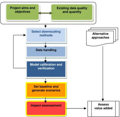
The IPCC document “Guidelines for Use of Climate Scenarios Developed from Statistical Downscaling Methods” presents an overview on statistical downscaling methods (Wilby et al., 2004). The general scheme for obtaining climate scenarios using downscaling approaches is summarized in
Figure 2.1
.Figure 2.1 – Main steps in obtaining and using downscaled climate scenarios by way of statistical approaches. Project aims and
objectives
Existing data quality and quantity
Select downscaling methods
Data handling
Model calibration and verification
Set baseline and generate scenarios
Assess value added Alternative approaches
When opting for a statistical method approach it is important to assess model errors by comparing the climate simulations with independent observed climate. For example, if the observed dataset for the 1971-1990 period is used for model construction, then the same dataset must not be use to validate the simulations. An independent data such as the 1991-2000 dataset is preferred for validation. This step is very important to define if the simulations are representative or not of the local climate variability and if the statistical methods can be applied.
Alternative methods such as using Global Circulation Models to assess climate change at higher spatial resolutions can be applied, but this approach usually don’t represent local climate variability, for example, specific microclimates or costal zones, orographic precipitation and islands. The following sections will give an overview on the state of the art of different downscaling methods available.
2.1 Dynamical Downscaling
Dynamical downscaling is based on numerical simulations of physical atmospheric and ocean processes operating in nature, involving the nesting of a higher resolution Regional Climate Model (RCM) within a coarser resolution GCM. The RCM uses the GCM to define time–varying atmospheric boundary conditions around a finite domain, within which the physical dynamics of the atmosphere are modeled using horizontal grid spacing’s (Grotch and Maccracken, 1991).
Most of today’s regional climate models (e.g. CHRM1, HadRM2, HIRHAM3) have spatial
resolution between 20 and 60 km and are able to simulate regional climate features such as orographic precipitation, regional scale microclimates and some extreme events.
A growing number of studies are being published, comparing the ability of RCMs to simulate climate variables, particularly those relevant for hydrological studies. In general, RCMs behave well in respect to temperature related statistics such as mean monthly values, but demonstrate problems when representing some features of precipitation. For instance, Pan
et al. (2001) evaluated the uncertainties of two regional climate models, at the spatial resolution of 50 km, with realistic orographic precipitation, east-west transcontinental gradients and with reasonable annual cycles over different geographic locations. In this case, both models behaved well in respect to temperature, but failed when representing
extreme precipitation events. Another similar analysis conducted by Dankers et al. (2007), for the regional climate model HIRHAM at the spatial resolutions of 12 km and 50 km, showed that the higher resolution simulations presented good results for orographic precipitation patterns and extreme rainfall events. But again, the average precipitation rates were generally higher than observed, while extreme precipitation levels were mostly underestimated.
A comparison study of ten RCMs developed by the European Project PRUDENCE4
concluded that most of the uncertainties sources of RCMs do vary according to the spatial domain, region and season. However, it was also concluded that the role of boundary forcing, i.e. the choice of the driving GCM, has generally a greater role on the sources of uncertainty than the RCM used, in particular for temperature (Deque et al., 2007).
Since the mid nineties local adaptation and mitigation measures of global warming started to be considered. The need to support this type of policy making with objective and more accurate data lead to the necessity of improving and developing new dynamical downscaling methods and prompted many model comparison and validation studies. In 1997 the Project MERCURE5 (Modelling European Regional Climate, Understanding and
Reducing Errors) established five main goals to overcome and understand models errors and uncertainties. Those goals were: (i) to understand the sources of errors that hinder the representation of physical processes; (ii) to improve the representation of the hydrological cycle; (iii) to assess the ability of regional models to reproduce observed precipitation frequency; (iv) to characterize errors in regional climate simulations nested in general circulation models; and (v) to provide statistical-dynamical tools linking RCM and GCM simulations, overcoming and understand RCMs uncertainties (Busch and Heimann, 2001).
There has been a strong effort to perform and release to the scientific community more regional climate models simulations carrying less uncertainty. However, this continues to be computationally expensive, so this goal is still distant. In fact existing RCMs runs are usually restricted to one or two climate change scenarios for a limited area, and for limited time periods; usually 30 years for a control baseline climate, viz. 1961-1990.
4PRUDENCE - Prediction of Regional scenarios and Uncertainties for Defining EuropeaN Climate change risks
and Effects. (http://prudence.dmi.dk/)
5MERCURE - Modelling European Regional Climate, Understanding and Reducing Errors.
The regional climate model PRECIS6 (Providing REgional Climates for Impacts Studies) was
developed by the Hadley Centre to help generate high resolution climate change information, based on the Hadley Centre’s regional climate modelling system, and its main innovation was that it can run in a regular PC under the Linux operating system. It is an excellent technological advance but still has some important limitations. For example, a typical experiment, covering a 100-by-100 grid-box domain including a representation of the atmospheric sulphur cycle run on a 2.8 GHz machine, takes up to 4.5 months to complete a 30 year simulation (UNDP, 2003).
However it can be expected that this type of technology will become faster and simpler to use in the coming years, enabling smaller teams and even specialists from other fields to perform their own dynamic downscaling of global warming impacts for different periods, scenarios and geographical locations.
2.2 Statistical Downscaling
One simple method of assessing climate change at a local scale is to apply GCM projections in a form of change factors (CFs) usually called the “delta-change” approach (Fowler, et al. 2007). In this method, first, baseline climatology is established for a specific area or region; e.g. 1961-1990 averages of daily temperature and daily precipitation sum. Secondly, the changes from the GCM or RCM, for the grid box that includes the meteorological station, between the same baseline period and the future scenario are determined. Finally, those changes are applied to the baseline time series. For example; if the temperature difference between the 2060-2090 GCM scenario and the GCM baseline is 2ºC, then 2ºC are added to the daily temperature dataset. This simple method does not take into account the variability, only scaling the mean, maxima and minima of climate variables, assuming that the spatial pattern will remain the same in the future. These limitations are more significant in precipitation when ignoring the length change of wet and dry spells that are very important in climate change studies (Diaz-Nieto and Wilby, 2005).
Alternatively, statistical downscaling (SD) models relay on the fundamental concept that regional or local climate strongly depends on larger scale atmospheric variables (such as mean sea level pressure, geopotential height, wind fields, absolute or relative humidity, and temperature variables). This relationship can be expressed as a deterministic and/or stochastic function of the large-scale atmospheric variables (predictors) and regional or local
climate variables (predictands) like temperature. One of the main weaknesses of the SD methods is that the output is generated for a single-site that can, or not, represents the entire study area. Applying SD methods for multisite can be time consuming while using CFs for all meteorological stations in the study area is very easy to accomplish.
There are several SD methods and approaches that can be used to generate climate change scenarios at a local scale. Without going too deep on the subject SD methods can be grouped in three categories: Weather typing schemes, regression models and weather generators. In the first category, weather patterns are grouped according to their similarity and the predictand is then assigned to the prevailing weather state, and replicated under climate changed conditions (Corte-Real et al., 1999). Regression models include linear and non-linear relationships between predictands and large scale atmospheric forcing, like multiple regression, canonical correlation analysis and artificial neural networks. Finally, weather generators are simple stochastic models that replicate the statistical attributes of local climate and are used for downscaling by conditioning their parameters on large-scale atmospheric predictors, weather states or rainfall properties (Semenov and Barrow, 1997).
Huth et al. (2008) compared linear and non-linear methods for winter daily temperature at eight European stations. The linear methods included linear regression and the non-linear methods were represented by artificial neural networks. The results showed that the linear regression appears to be the best method but the neural networks showed better results on representing extreme or abnormal events. Another study conducted by Dibike and Coulibaly (2006) tested the use of temporal neural networks for downscaling daily precipitation and temperature, analyzing extremes in northern Quebec, Canada. In this case, the temporal neuronal network was generally the most efficient method for downscaling, especially on representing extreme precipitation and variability, outperforming the statistical models.
Statistical downscaling methods are continually evolving reproducing climate variability and extremes more and more accurately. Vrac et al. (2007) presented a new statistical downscaling approach combining large-scale upper-air circulation with surface precipitation fields, based on a non-homogeneous stochastic weather typing scheme. This method combined two different types of weather states; precipitation patterns and circulation patterns, improving important precipitation features like local rainfall intensities and wet/dry spell behavior.
Choosing the best method to produce climate change scenarios isn’t always straightforward. The application of SD methods assumes some knowledge on the relationship between local-climate and large scale atmospheric processes, even when statistical tools help choosing the best predictors from GCMs. Selecting the proper grid-box from the GCM can also be challenging. For example, the Tagus estuary in Lisbon, Portugal, is very close to four HadCM3 grid-boxes and the choice of one or multiple grid-boxes strongly depends on the sensitivity and local knowledge of climate variability as well as selecting the best correlation grid-box(es) for the predictor-predictand relationship.
There are several free statistical downscaling tools available for download on the internet but few offer a Graphical User Interface (GUI). For those who aren’t familiar with coding in fortran, MATLAB, C++, or other programming languages, a GUI comes in hand and helps performing the job almost intuitively. Nevertheless, it is fundamental to have some knowledge on statistics in order to select the best methods and the best predictor-predictand relationships.
Developed by Masoud Hessami, in collaboration with the “Centre Eau Terre Environnement Institut National de la Recherche Scientifique” (INRS-ETE) and the Environmental Canada, the Automated Statistical Downscaling (ASD) software is a hybrid of stochastic weather generator and regression-based downscaling methods that generates single-site scenarios of surface weather variables under current and future climate forcing (e.g. Hessami et al., 2008). It is also possible to find daily normalized predictor variables for the 1961-2001 period derived from the National Centre of Environmental Prediction (NCEP) reanalysis and the third generation Coupled Global Climate Model (CGCM3), for the A2 scenario experiment, developed by the Canadian Centre for Climate Modeling and Analysis (CCCMA).
climate change impacts using a robust statistical downscaling technique, performing ancillary tasks of data quality control and transformation, predictor variable pre–screening, automatic model calibration, basic diagnostic testing, statistical analyses and graphing of climate data. This software is also freely available at the SDSM web site (https://co-public.lboro.ac.uk/cocwd/SDSM/), and the statistical downscaling input, such as the HadCM3 predictors for the A2 and B2 scenarios, can be downloaded from the Canadian Climate Change Scenario Network web site (http://www.cccsn.ca). Both format and extensions of the predictors files are compatible with the ASD and SDSM software.
Developed in Long Ashton Research Station by Mikhail Semenov,LARS-WG is a stochastic weather generator used for simulating weather for a single-site under both current and future climate conditions. This tool includes a new approach in simulating wet and dry spell length overcoming the limitations of the Marcov chain model of precipitation occurrence (Richardson, 1981). Instead of the predictor-predictand relationship, LARS-WG uses climate projections, such as precipitation, minimum temperature and maximum temperature, from GCMs and RCMs. The British Atmospheric Data Centre (BADC) holds the simulations from many models runs from several projects, including the results from the Climate Impacts LINK Project (http://badc.nerc.ac.uk/data/link/) containing both RCMs and GCMs climate projections for different emission scenarios of the UK Met Office Hadley Centre models, processed into text files at the Climate Research Unit at the University of East Anglia.
2.3 Statistical-dynamical downscaling
Some teams have large resources and expertise on meteorology, so they hold the ability to supply others with high resolution climatic data. For these teams, deciding whether to use a statistical or a dynamical downscaling method to assess climate change scenarios can be challenging. For some areas a dynamic method simply can’t be used by lack of adequate data for input, calibration and validation.
downscaling over Spain during four seasons did not reach any conclusion on which would be the best method, as results varied depending on the specific season and region.
Also, the IPCC Fourth Assessment Report (2007), quoting results from the European Projects PRUDENCE (dynamical downscaling) and STARDEX7 (statistical downscaling),
remarks that none of the different techniques surveyed was clearly superior: to obtain better results and a quantification of uncertainties, the best way was to use and compare them all. Of course, this is not feasible when working on scientific projects where the main object of research is not climate itself.
In this context of the state-of-the-art, combining statistical and dynamical methods has become a priority for the next generation of climate downscaling methods. Projects like ENSEMBLES8, UKCIP089 and NARCCAP10 are advancing along this path, combining the
state-of-the-art, high resolution, global and regional Earth System models, to produce objective probabilistic estimates of future climates.
7STARDEX - Statistical and Regional dynamical Downscaling of Extremes for European regions.
(http://www.cru.uea.ac.uk/projects/stardex/)
8ENSEMBLES – Ensembles-Based Predictions of Climate Changes and Their Impacts.
(http://ensembles-eu.metoffice.com/index.html)
3 IMPLEMENTATION OF STATISTICAL DOWNSCALING METHODS TO A
SINGLE SITE IN LISBON
3.1 Case study description
For the case study it was chosen to apply two different statistical downscaling methods for a single site in Lisbon. The first method is a stochastic weather generator that can be use for the simulation of weather for a single site under current and future climate conditions. This method was applied using the LARS-WG (Long Ashton Research Station Weather Generator) tool developed by Semenov and Brooks, (1999) that provides means of simulating synthetic weather time series with similar statistical characteristics of the observed statistics at a site.
The second statistical downscaling method is a hybrid of stochastic weather generator and transfer function methods. In this case, large-scale circulation patterns and atmospheric moister variables are used to condition local scale weather parameters such as precipitation occurrence and intensity. Stochastic techniques are then used to artificially inflate the variance of the downscaled daily time series. This method was applied using the SDSM (Statistical DownScaling Model) tool developed by Wilby, Dowson and Barrow, 2001.
The climatic inputs for both statistical methods was daily precipitation, daily maximum temperature and daily minimum temperature for Lisbon during the 1961-1990 period, obtained from the European Climate Assessment & Dataset (ECA&D) for the following meteorological station: Name: 177 LISBOA GEOFISICA; WMO: 08535; Latitude: 38:43:00; Longitude: -09:09:00; Height: 77m.
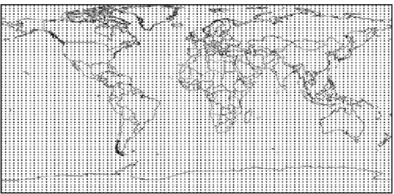
Figure 3.1 – GCM HadCM3 global grid (96x73); each point represents the centre of the grid box. The HadCM3 GCM covers the IPCC following criteria’s (IPCC, 2001):
• full 3D coupled ocean-atmospheric GCMs,
• documented in the peer reviewed literature,
• has performed a multi-century control run (for stability reasons),
• has participated in CMIP2 (Second Coupled Model Intercomparison Project),
• has performed a 2 x CO2 mixed layer run,
• has participated in AMIP (Atmospheric Model Intercomparison Project),
• has a resolution of at least T40, R30 or 3º latitude x 3º longitude, and
• considers explicit greenhouse gases (e.g. CO2, CH4, etc.)
For this study the GCM HadCM3 daily data were collected in two different sources. The predictors for the A2 scenario used in the SDSM tool were acquired at the Canadian Climate Change Scenarios Network (CCCSN), and the input for the LARS-WG tool were collected at the British Atmospheric Data Centre, from the Climate Impacts LINK Project.
The following sub-chapters describe how these tools were implemented and also how to acquire observed and simulated future daily data for climate scenarios.
and was compared with the observed statistics in January using 31x10=310 values. An uncertainty analysis was also performed using a non-parametric bootstrapping technique comparing both model simulations with thirty years of observed climate. For example, the uncertainties analysis for January were calculated using 31x30=930 values and compared with 31x30=930 values from the simulations for each climate variable.
Finally, in chapter 5, it was simulated one climate change scenario (A2 SRES scenario) was simulated producing daily datasets for each climate variable for the 2041-2070 period for a single site in Lisbon.
3.2 Baseline meteorological data
Using statistical downscaling methods strongly depends on the quantity and quality of available local meteorological data. Getting some decades of daily precipitation and temperature data for a certain reference meteorological station is often no easy task, but is indispensable for model calibration and validation.
Usually model calibration and validation is done with thirty years of daily meteorological records, often from 1960 to 1990. Most of the observed predictors for model calibration also correspond to the 1960-1990 period allowing the establishment of the predictor-predictand relationships that provide the basis for producing climate change scenarios when using statistical downscaling models.
Local climate data can often be obtained from national meteorological institutes, but other institutions hold valuable weather data such as airbases, universities, public laboratories, governmental institutes in charge of water resources, forests, agriculture and air quality. Although it is becoming more frequent to have that information freely available online, in many cases one must expect that a payment will be asked for, at least for covering data processing costs.
3.3 Climatic data for future scenarios
Since the IPCC Third Assessment Report in 2001 a growing number of projects where conducted to determine the impact of climate change at a regional and local scale. One example is project PRUDENCE (Prediction of Regional scenarios and Uncertainties for Defining EuropeaN Climate change risks and Effects), which is part of a co-operative cluster of projects exploring future changes in extreme events in response to global warming, together with Projects such as STARDEX (STAtistical and Regional Downscaling of EXtremes) and MICE (Modelling the Impact of Climate Extremes). The simulation results from different model runs of seasonal, monthly and daily datasets for the A2 and B2 scenarios and for the period of 2070 to 2100 can be downloaded from the PRUDENCE web page (http://prudence.dmi.dk/). The files are in the NetCDF (network Common Data Form) format; which is a set of interfaces for array-oriented data access with a freely-distributed collection of data access libraries for C, Fortran, C++, Java, and other languages.
The North American Regional Climate Change Assessment Program (NARCCAP) is also producing high resolution climate change scenarios for the United States, Canada, and northern Mexico, investigating uncertainties in regional scale projections of future climate. The simulation results (A2 scenario from 2041 to 2070 with 50 km spatial resolution) are downloadable from the Earth System Grid web page (www.earthsystemgrid.org).
3.4 LARS-WG: a stochastic weather generator
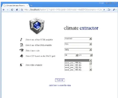
Since the data extraction process can be very repetitive and laborious, a web based interface was developed in Active Server Pages (ASP) programming language that extracts and produces text files with time series for any grid box chosen automatically. Figure 3.2 shows how this climate extractor looks like.
Figure 3.2 – Web based tool to extract global climate data to one chosen grid box.
LARS-WG can generate synthetic daily datasets of precipitation, minimum and maximum temperature and solar radiation based only on one year of observed weather, but, as mentioned before, it is recommended to have 20 or 30 years of daily climate data in order to capture real climate variability and seasonality. This process can be divided in three distinct steps: (i) site analysis, (ii) model validation and (iii) generation of synthetic weather data.
3.4.1 Site Analysis
The goal of this first step is to do a preliminary analysis of the observed dataset to exclude some errors that can occur like, minimum temperature higher than maximum temperature and negative precipitation values. This step as to be done for the observed period, the GCM baseline period and the GCM future scenario (e.g., 2041-270 to represent the 2050s).
3.4.2 Model validation
Model validation is one of the most important steps of the entire process and the objective is to assess the model performance to simulate climate at the chosen site in order to determinate whether or not it is suitable for use. The model construction was based on the observed daily dataset from 1961 to 1980 and the validation was preformed using the observed daily dataset from 1981 to 1990.
During this step, a 30 year simulation of daily precipitation and daily maximum and minimum temperature was done, and the model errors in the estimates of means and variances were evaluated using non-parametric statistical hypothesis tests at the 95% confidence level. The results from this process are shown in chapter 4.
3.4.3 Creating climate change scenarios
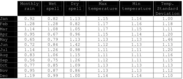
To incorporate changes in climate variability and generate scenarios, the relative change between the GCM baseline period and the GCM future scenario was calculated. Parameters calculated were: relative change in wet and dry series length; relative change in mean temperature standard deviation for each month; and mean changes in precipitation amount, mean temperature and solar radiation for each month. For example, to calculate the relative change between the baseline period and future scenario of the monthly rain in January, the average of the total monthly rain in January for the future scenario (2041-2070 period) was divided by the average of the observed total rain in January for the 1961-1980 period. Table 3.1 shows the relative change matrix used for the A2 scenario.
Table 3.1– Relative change (SCENARIO/BASELINE) between the GCM future scenario (2041-2070) and GCM baseline period using the daily dataset.
Monthly rain
Wet spell
Dry spell
Max temperature
Min temperature
Temp. Standard Deviation
Jan 0.92 0.82 1.13 1.15 1.14 1.00
Feb 1.28 1.28 0.82 1.17 1.16 1.18
Mar 1.14 1.08 1.05 1.17 1.15 1.11
Apr 0.95 0.67 0.96 1.15 1.14 1.20
May 0.65 0.79 1.13 1.13 1.13 1.46
Jun 0.72 0.84 1.42 1.12 1.13 1.13
Jul 1.14 1.26 0.98 1.11 1.11 1.20
Aug 0.83 1.06 1.15 1.11 1.11 1.16
Sep 0.56 0.75 1.26 1.12 1.11 1.15
Oct 0.77 0.85 1.09 1.13 1.13 1.13
Nov 0.95 0.87 0.86 1.13 1.13 1.12
The changes in mean temperature are additive changes, and changes in monthly precipitation, length of the wet and dry spells and temperature standard deviation are multiplicative. For example, in this study the wet spell relative change in August, for the 2041-2070 period was 1.06, meaning that for each length of the wet spell chosen by LARS-WG for August will be multiplied by 1.06 when creating the new synthetic dataset.
3.5 SDSM: a multi-regression model
SDSM reduces the task of statistically downscaling weather series into five steps: (i) quality control and data transformation; (ii) screening of predictor variables; (iii) model calibration and selection; (iv) model validation; and (v) scenario generation from GCM predictors.
SDSM uses predictors, such as mean sea level pressure and geopotential height, that can be downloaded from the NCEP/NCAR reanalysis project web site (http://www.cdc.noaa.gov/cdc/data.ncep.reanalysis.html). For this particular study the datasets where already pre-prepared and downloaded from the Canadian Climate Change Network (http://www.ccsn.ca/). These datasets also derived from the NCEP reanalyzes but where firstly interpolated to the same grid as HadCM3 GCM (2.5º latitude x 3.75º longitude) and then normalized over the complete 1961-1990 period.
3.5.1 Quality control and data transformation
During this step it is important to check for data errors, missing codes and outliers. Some times is also needed to apply data transformation specially when there are a lot of zero values and large numbers in the same dataset. Some of the most common transformations are: logarithm, power, inverse, lag and binomial. For this study only the precipitation data was transformed using a fourth rout transformation.
3.5.2 Screening of downscaling predictor variables
The main goal of this step is to establish the relationships between predictors and a single site predictand. This selection was based on the observed time series for the 1961-1980 period.
The first criteria were applied based on local knowledge and inter-month climate variability in Lisbon. To have a better representation of seasonality a different model for each month was built based on different predictor-predictand relationships.
Thirdly, to test the significance of the predictor-predictand relationship it was calculated the correlations at the 95% confidence interval. The predictor-predictand process is when a specific variable is dependent or not on other variables. For example, when the predictand is not regulated by an intermediate process, such as the case of minimum and maximum temperature, it must be use an unconditional process, when the predictand is regulated by an intermediate process, such as the case with precipitation were the amounts depend on the wet-day occurrence, the conditional process must be used.
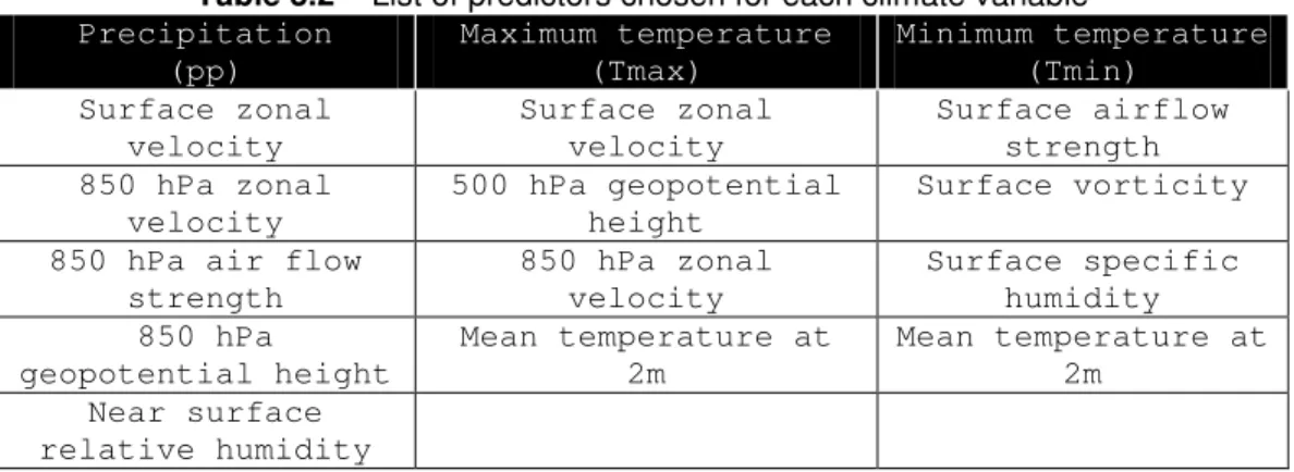
Finally, to smooth the inter-monthly curve, an autoregressive term was used. This process is very common when modeling time series. The predictors chosen for each climate variable are presented in Table 3.2.
Table 3.2 – List of predictors chosen for each climate variable Precipitation (pp) Maximum temperature (Tmax) Minimum temperature (Tmin) Surface zonal velocity Surface zonal velocity Surface airflow strength 850 hPa zonal
velocity
500 hPa geopotential height
Surface vorticity
850 hPa air flow strength
850 hPa zonal velocity
Surface specific humidity 850 hPa
geopotential height
Mean temperature at 2m
Mean temperature at 2m
Near surface relative humidity
3.5.3 Model calibration and selection
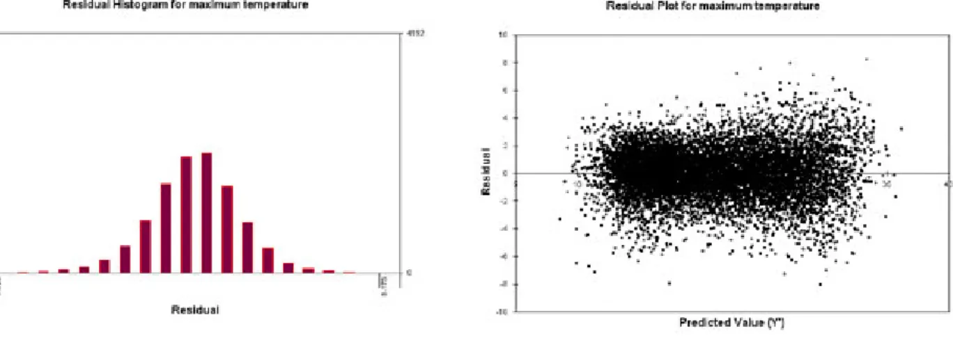
Model calibration was done to improve the models results for the predictor-predictand relationship by doing a sensitivity analysis on the steps 3.5.1 and 3.5.2. After selecting the most suitable predictor variables the model based on multi-regression equation was applied and the selection of the best model was based on checking the normality, homogeneity and independence assumptions by plotting a histogram of the residuals, the residuals versus the predicted variable and calculating the Durbin-Watson statistics to respectively assess each assumption.
is desirable to have the spread uniformly distributed and without patterns, which means there is no violation of homogeneity. The Durbin-Watson statistic is a statistical test used to detect the presence of autocorrelation in the residuals from a regression analysis. A value of 2 indicates there appears to be no autocorrelation; if less than 2, there is evidence of positive serial correlation and a rough rule of thumb could be applied, if Durbin–Watson is less than 1.0 is very probable that we have auto correlation and the independence assumption is violated. The following figures (Figure 3.3, 3.4, 3.5, 3.6, 3.7 and 3.8) and tables (Table 3.3, 3.4, 3.5) show these results for the selected models.
Figure 3.3
-
Histogram of the residuals to check normality for the maximum temperature model.Figure 3.4 – Residuals vs predicted value to check homogeneity for the maximum temperature model.
Table 3.3 – Coefficient of determination R2 and Durbin-Watson statistics for validating the independence assumption for the maximum temperature model.
Jan Feb Mar Apr May Jun Jul Aug Sep Oct Nov Dec
R2 0.468 0.504 0.698 0.707 0.776 0.747 0.666 0.609 0.733 0.726 0.622 0.534
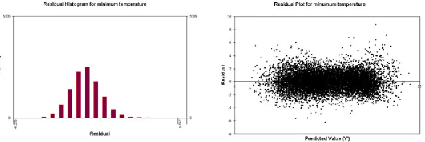
Figure 3.5 – Histogram of the residuals to check normality for the minimum temperature model.
Figure 3.6 – Residuals vs predicted value to check homogeneity for the minimum temperature model.
Table 3.4 – Coefficient of determination R2 and Durbin-Watson statistics for validating the independence assumption for the minimum temperature model.
Jan Feb Mar Apr May Jun Jul Aug Sep Oct Nov Dec
R2 0.641 0.682 0.668 0.668 0.675 0.700 0.590 0.505 0.663 0.674 0.699 0.711
Durbin-Watson 1.878 1.871 1.732 1.776 1.773 1.891 1.809 1.913 1.913 1.878 1.815 1.803
Figure 3.7 – Histogram of the residuals to check normality for the precipitation model.
Figure 3.8 – Residuals vs predicted value to check homogeneity for the precipitation model.
Table 3.5 – Coefficient of determination R2 and Durbin-Watson statistics for validating the independence assumption for the precipitation model. [n.a. = not available]
Jan Feb Mar Apr May Jun Jul Aug Sep Oct Nov Dec
R2 0.447 0.435 0.416 0.399 0.405 0.344 0.123 0.204 0.336 0.477 0.452 0.474
The residual analysis showed in the previous tables (Table 3.3, 3.4, 3.5) and plots (Figure 3.3, 3.4, 3.5, 3.6, 3.7 and 3.8) demonstrate that there is no violation of normality, homogeneity and independence assumptions. Unfortunately the SDM tool was unable to calculate the Durbin-Watson statistics for conditional models and the independence assumption was not confirmed for precipitation. Also the spread of the residuals versus observed precipitation plot shows some lines of points. That is due to the large number of zero of the observed precipitation.
3.5.4 Model validation
Model validation was performed by simulating synthetic time series of daily precipitation and daily maximum and minimum temperature for 30 years and compared with observed daily precipitation and daily maximum and minimum temperature for the 1981-1990 period.
The model errors in the estimates of means and variances were evaluated using non-parametric statistical hypothesis tests at the 95% confidence level.
All outliers that represent unusual phenomena’s, trends or variations that were not typical were removed from the 1961-1990 observed dataset in order to have a representation of the normal climate behavior and variability. The comparative results for model validation are presented in detail in chapter 4.
3.5.5 Scenario generation from GCM predictors
4 MODEL VALIDATION AND UNCERTAINTY ANALYSIS OF LARS-WG AND
SDSM SIMULATIONS FOR THE CASE STUDY
The model validation and uncertainty analysis in downscaled daily precipitation and daily maximum and minimum temperature (Tmax and Tmin respectively) was assessed in terms of model errors in the estimates of the mean and variances for the 1981-1990 period and confidence intervals in the estimates of means and variances for the 1961-1990 period. This analysis was conducted in three main steps: exploratory analysis of the observed dataset to decide either to use a parametric or non-parametric approach in step one; models errors analysis with statistical significance tests at 95% confidence level; and finally in step three, the confidence intervals of the estimates of means and variances of the observed and downscaled data were estimated using a bootstrap non-parametric approach.
The following subsections describe some background information used in the uncertainty assessment.
4.1 Exploratory analysis
Many statistical methods depend on the assumptions that the data have a nearly normal distribution and are uncorrelated when collected over regular time periods. If these assumptions are not verified the classical statistical methods may be misleading and a non-parametric approach produces more robust results.
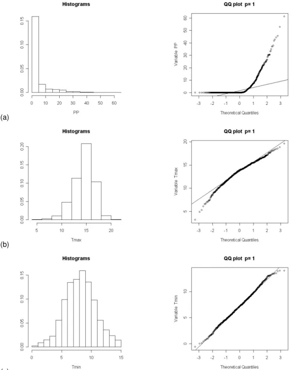
To assess these assumptions a graphical analysis was preformed by looking at the following collection of plots for the 1961-1990 period: histograms and normal quantile-quantile (QQ) plots. A histogram shows the centre and distribution of the data giving an indication of normality. The QQ-plot is a graphical tool used to determine whether the data follow a particular distribution comparing it to the Gaussian distribution. If the resulting points lie on a straight line, then the distribution of the data is considered to be the same as a normally distributed variable.
The exploratory data analysis of the observed daily temperature (Tmax and Tmin) and daily precipitation (PP) for January at the “Lisboa Geofísica” meteorological station for the 1961 to 1990 period are shown in Figure 4.1.
(a)
(b)
(c)