HEALTH EXPENDITURES‟ COPING STRATEGIES
A study on African low-income countries
Sara Isabel Ferreira Mendes, number 269
A Project carried out with the supervision of: Professor Pedro Pita Barros
Abstract
In the absence of formal coping mechanisms in the face of health expenditures, households are forced to penalize their resources and to use one or more strategies. Those strategies include using own resources, selling assets or borrowing from others outside the household. We show that different factors influence how families in developing countries cope with health spending.
Given the data available, the study identifies the relevant factors to recognize households in financial distress due to health expenditures. Their fragile position is proven to be mainly characterized by the size of the family, educational level, location of the household and asset ownership quintile.
Key Words: health; expenditures; coping strategies; Africa.
Acknowledgments: This paper uses data from the WHO World Health Surveys. We
Section 1. Introduction
Income and expenditure shocks play a key role in determining welfare in the developing world. In many developing countries, people are expected to pay on its own the cost of health care. Therefore, their ability to pay for health care has become a significant policy issue. “ The money used to pay for health care may otherwise have been used for food, agricultural development or education. Payment for health services is thus made at considerable social cost to the family and can scarcely be said to
represent a “willingness” to pay in the normal sense of the word.” (Russell, 1996, p.1)
From previous literature, common household responses to payment difficulties are identified, ranging from borrowing to more serious 'distress sales' of productive assets and, eventually, abandonment of treatment.1
In designing their health systems, policy makers need to understand whether some characteristics make people more exposed to catastrophic payments.
In that sense, the aim of this work project is to identify which households are more vulnerable and to explore the impact that several factors have on influencing the choice of strategies to cope with health expenditures. The strategies adopted include not only the use of own resources but also the possibility of selling assets and borrowing from others. Factors that may influence the household behavior range from socioeconomic characteristics to the percentage of dependent members and asset ownership level.
Families‟ vulnerability was found to be directly related to their size, educational
level and members in a poor health status. Moreover, households at the lowest quintiles
1
tend to be more expose to use penalizing strategies when facing health expenditures than people in the highest quintiles.
Expenditure is defined as catastrophic if a household‟s financial contributions to the health system exceed 40% of income remaining after subsistence needs have been met (Xu et al., 2003). High health care costs may not be reflected in catastrophic expendituresif the household does not bear the full cost because the service is provided free or at a subsidized price, or is covered by private insurance. On the other hand, for poor households even small costs can lead to financial disaster.
Thus, whereas financial protection against events of illness is increasing among the insured population, the non-insured do not have such protection and are, therefore, at a greater risk of incurring in catastrophic expenditure. If they fall ill, the related expenses have to be covered through out-of-pocket payments. The poor have very little access to formal insurance. In many surveys, questions about insurance are not even asked. When the poor come under economic stress, their form of “insurance” is often
eating less or taking their children out of school. Ultimately, informal insurance relies on the willingness of the fortunate to take care of those less favored. Unfortunately governments in these countries are not very effective at providing insurance either. For example, in most countries, the government is supposed to provide free health care to the poor. Yet, health care is rarely free. (Banerjee and Duflo, 2006)
Section 1 will introduce the subject and purpose of the study, Section 2 will revise past contributions to the area, while Section 3 will enlighten about the methodology used. Sections 4 and 5 will determine which factors influence the most the probability of using each of the available strategies and the existence of health expenditures. Finally, Section 6 will point out the limitations of this study and the economic insights of the results.
Section 2. Literature Review
Health shocks
The economic consequences of health shocks in developing countries have been the focus of increasing attention. Health shocks are defined as unpredictable illnesses that diminish health status.
When faced with a health shock households often incur in catastrophic expenditures. A health shock can lead to financial hardship and even impoverishment. Many of those who do seek care suffer financial catastrophe and impoverishment as a result of meeting these costs, the financial consequences of paying for care (Xu et al., 2007). The term catastrophic implies that such expenditure levels are „„likely to force
households to cut their consumption of other minimum needs, trigger productive asset sales or high levels of debt, and lead to impoverishment‟‟ (Russell, 2004, p.147).
In fact, health insurance, either public or private, is exceptional in the majority of developing countries and correspondingly, much of the borrowing and saving by households is of informal nature. The households are generally characterized by their lack of collateral that restraint them to access to credit markets.
Out-of-pocket payments
Out-of-pocket health payments refer to the payments made by households at the point they receive health services. Typically these include doctor‟s consultation fees,
purchases of medication and hospital bills. It is also important to note that out-of-pocket payments are net of any insurance reimbursement (Xu et al., 2005).
In absence of formal health insurance, it is argued that the strategies households adopt to finance health care have important implications for the measurement and interpretation of how health payments impact on consumption and poverty (Flores et al., 2008). Although most of the variation in catastrophic spending can be explained by the triad of poverty, health-service use, and the absence of risk pooling mechanisms, important unexplained variation remains (Xu et al., 2003).
The analysis lead us to think that if out-of-pocket spending could be reduced to levels lower than a threshold level of total health spending, few households would be affected by catastrophic payments. The cross-country variation, however, often shows that other more complex strategies can protect households against catastrophic spending, such as progressive fee schedules, highly subsidized or free hospital services, and the provision of certain health services to the poor (Xu et al., 2003). Moreover, the incidence of financial catastrophe is negatively correlated with the extent to which countries fund their health systems using prepayment of some form - taxes or insurance. Conversely, catastrophe is positively correlated with the relative importance of out-of-pocket payments in total health spending (Xu et al., 2007).
Coping with health expenditures
land or livestock in a rural setting, often increasing a vicious cycle of increased economic vulnerability. The most common response is, however, borrowing, from family and friends, highlighting the importance of social networks, or from a money-lender. Other strategies for dealing with the direct costs of illness include diversifying income by engaging in activities other than their normal work or households selling their labor (Sauerborn et al., 1996). The response to health shocks is extremely influenced by household relationships‟ structure and between the household and their social networks. Social connections end up playing an important role in the availability of loans and in the respective settlement of interest rates.
In fact, using income and savings, borrowing or selling assets are driven by different motivations and in that sense treated as separate strategies as opposed to out-of-pocket payments described in the studies mentioned above. Further in this analysis are not only presented the factors that influence coping mechanisms but also the ones that influence having health expenditures, when there is no protection towards an health shock.
Section 3. Methodology
3.1 Characterization of the Sample
spread throughout the western, central, eastern and southern parts of sub-Saharan Africa.
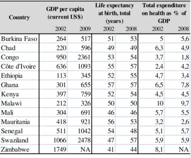
These countries differ in their levels of income, life expectancy and total health expenditure. In 2002, the GDP per capita varies a lot between the countries in the sample, being the lowest value attributable to Ethiopia (US$ 113) and the highest to Zimbabwe (US$ 1749). The life expectancy ranges from 41 years in Zimbabwe to 57 in Ghana. Total expenditure on health as a percentage of GDP was less than 6% except in Chad, Ghana, Malawi and Zimbabwe.
Table 1. Gross Domestic Product per capita, Life expectancy and Total expenditure on
health as proportion of GDP:
In 2009, the lowest GDP per capita is now attributed to Malawi (US$ 326) and the highest to Swaziland (US$ 2478) being Ethiopia the country with the highest growth of GDP per capita during this period and Malawi with the lowest. The data available for
2002 2009 2002 2008 2002 2008
Burkina Faso 264 517 51 53 5 5,6
Chad 220 596 49 49 6,3 4,9
Congo 950 2361 53 54 3,7 1,8
Côte d'Ivoire 636 1093 55 57 2,4 4,2
Ethiopia 113 345 52 55 4,7 3,4
Ghana 301 655 57 57 6,5 7,8
Kenya 397 759 52 54 4,5 4,5
Malawi 212 326 50 50 10 9,7
Mali 304 691 46 46 5,7 5,5
Mauritania 418 921 56 53 3,2 2,6
Senegal 511 1042 54 48 5,1 5,7
Swaziland 1066 2478 47 57 5,9 5,9
Zimbabwe 1749 NA 41 44 8,1 NA
S o urc e : Wo rld B a nk a nd Na tio na l He a lth Ac c o unts o f Wo rld He a lth Orga niza tio n, 2002. Country
GDP per capita (current US$)
Life expectancy at birth, total
(years)
Total expenditure on health as % of
GDP
these countries on life expectancy and total expenditure in health as a percentage of GDP is from 2008; their relative and absolute position did not change significantly.
The health systems of these countries are generally characterized by low level of revenues coming from the government, low total health spending and few risk-pooling mechanisms. Private financing sources are generally firms, NGOs, households or other entities (predominantly funding from external resources).
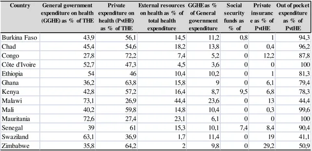
Total expenditure on health aggregates both public and private spending on health. The percentage of the expenditure on health financed by the private sector is higher than the percentage financed by public contributions for the majority of the countries. Public outlays on health include tax-funded health expenditure, Social Security and External Resources. The percentage of total health expenditure that External Resources finance ranges from 2% in Zimbabwe to 44.4% in Malawi. External Resources are loans and grants for medical care and medical goods channeled through the Ministry of Health or other public agencies. Grants to non-governmental organizations are accounted for as private expenditure but, in practice, they are not always easily separated from public grants.
Social Security on Health is the premiums paid by employees and employers for compulsory schemes of medical care and medical goods for a sizeable group of population, which have no contribution almost in all countries, being Kenya and Senegal the exceptions.
spending is direct payments of households for goods and services whose primary intent is to contribute to the restoration or to the enhancement of their health status. These include the payments made to public services, profit institutions or non-governmental organizations by households.
As a share of private health expenditure, out-of-pocket payments range from less than 41.1% in Swaziland to about 100% in Cote d‟Ivoire and Mauritania, with an
average of about 80% for the 13 countries. Some of the countries, such as Burkina Faso, Ghana and Senegal, have community health insurance, mostly working through microfinance initiatives, since social health insurance why exists in a small number of African countries.
Table 2. National Health Accounts 2002.
Country General government expenditure on health (GGHE) as % of THE
Private expenditure on health (PvtHE) as % of THE
External resources on health as % of
total health expenditure
GGHE as % of General government expenditure Social security funds as % of GGHE
Private insuranc e as % of
PvtHE
Out of pocket expenditure
as % of PvtHE
Burkina Faso 43,9 56,1 14,5 11,2 0,8 1 94,3
Chad 45,4 54,6 18,2 13,8 0 0,4 96,2
Congo 27,8 72,2 7,4 5,2 0 12,2 87,8
Côte d'Ivoire 52,7 47,3 4,5 3,6 0 0 100
Ethiopia 54 46 10,4 10,2 0 1 81,3
Ghana 36,2 63,8 15,8 9 0 6,1 79,4
Kenya 42,8 57,2 16,4 8,7 9,5 6,8 78,3
Malawi 73,1 26,9 44,4 23,6 0 13 44,4
Mali 40,2 59,8 14,8 10,4 0 0,3 99,6
Mauritania 72,6 27,4 23,1 6,1 0 0 100
Senegal 39 61 15,3 10,1 7,4 8,4 90,4
Swaziland 63,1 36,9 1,7 11,4 0 19 41,1
Zimbabwe 35,8 64,2 2 9,8 0 29,2 50,9
3.2 Data
The data was obtained from the World Health Survey conducted in 2002–2003, which was launched by the World Health Organization.2 The World Health Survey is cross-sectional and is based on a multi-stage clustered random sample of households designed to be nationally representative. The questionnaire is standardized across countries.3
The survey collects a range of information on health service utilization, expenditures and household socioeconomic indicators. The household questionnaire is administered to the household member most knowledgeable about the household. The information used from the survey includes socioeconomic information about household members such as gender, age, level of education and occupation, as well as households assets, health expenditures and behaviors on coping with the latter.4
Particularly, household expenditures were collected for a four-week recall period and the sources that are used to pay any health expenditure were collected for a year recall period. Such sources include income, savings, payment or reimbursement from a health insurance plan, sold items, family members and friends outside the household, borrowed from someone else and other.
The households that benefited from private insurance coverage were excluded from the sample analyzed. This exclusion is justified by the fact that the households with insurance coverage were in some way protected towards a health shock and in that sense in a different process of decision making in terms of how to finance their health
2
More information can be obtained at http://www.who.int/healthinfo/survey/whsresults/en/index.html
3
Questionnaire specific for low-income countries.
4
expenditures. With this exclusion 2% of the observations were lost, which accounts for a total of 1110 households with insurance. Country-wise, the proportion of losses ranges from 1% in Kenya Mauritania and Swaziland to 19% in Congo.5
3.3 Descriptive Statistics6
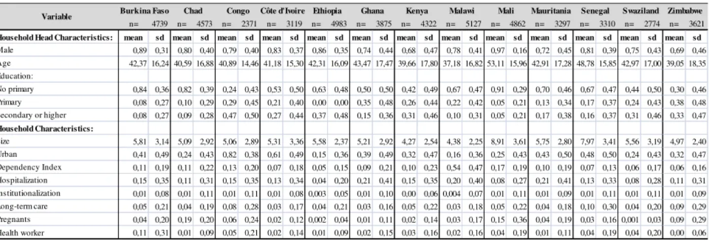
On average, 79% of the household heads are male, being the country with the highest percentage of male household heads Mali (with 97%) and the country with the lowest Zimbabwe (with 69%). The average age of the household head across countries is 43 years old, being the country with the highest average age Mali (with 53 years) and the lowest Malawi (with 37 years). In terms of education, the percentage of people not completing primary school ranges from 24% in Congo to 91% in Mali, while for having completed primary and more than secondary school the distribution is similar across countries, with an average proportion of 19% and 22%, respectively.
The average size of the households across countries in the sample is around 6 members, while Mali has the highest average, around 9 members and Kenya the lowest around 4 members. Additionally, in average 37% of the households are located in urban area, being Congo the country with a higher percentage of households in the urban areas (82%) and Ethiopia with more households located in the rural areas (15%).
The values of the dependency index range from an average value of 54% in Malawi to 5% in Ethiopia, while the percentage of having had hospitalizations range from 21% in Mauritania to 4% in Ethiopia. In terms of institutionalization of members the values did not differ much across countries, being around 1%. We observe the same
5
See Table A1, page 31.
6
behavior for the variables long-term care, pregnant women and health worker, with average values around 4%.
In addition, all of these countries were involved in conflicts in the African continent and suffered with many civil wars along the years. Particularly in the last decade, Chad and Kenya had two civil wars, while Côte d‟Ivoire, Mali and Senegal
suffered with only one civil conflict, respectively.
3.4 Empirical Methodology
Since each household can adopt a strategy or a combination of strategies of their choice, it is imperative to know the factors that influence not only the choice of each one of the three strategies separately but also the possible combinations. In the first case, the dependent variables analyzed include strategies that the households choose to cope with health expenditures, such as their own resources (income and savings), selling assets and borrowing.
Nevertheless, the existence of a relative importance of using a particular strategy is undeniable. Using own resources is less costly for the household than selling assets or even to be subject to a particular interest rate when borrowing from someone. As we do not have the information about in which proportions the households choose to follow each strategy, when combined, the choice of using the strategies will be also studied in ordinal terms.
ordinal scale. This variable assumes the value 1 when the household only uses its own resources to cope with health expenditure, 2 if the household uses not only the latter strategies but also sells their assets and finally 3 if the household uses all strategies available (if the household does not have savings or assets is also financial hardship if it borrows to cope with health expenditures). With penalization, the goal is to analyze which factors influence adoption of a coping strategy that implies a higher penalization of resources, an approach not taken in the previous literature.
Furthermore, when faced with the strategies that households can use to cope with health expenditures the importance of the existence of health expenditures arises. The reason is clear, a household without health expenditures does not face any constraint in defining which strategy to follow, being the existence of health expenditures the start of the process of decision making and the source of financial hardship for many households.
In order to study the factors that influence the existence of health expenditures the variable HE1 is built, a binary variable that takes the value 1 when the household had in fact any health expenditure and 0 otherwise.
The latter variable does not take into consideration an important feature when analyzing health expenditures in which households incur, its amount. In consequence, it was decided to create the fifth dependent variable studied, HE2 which assumes the values of the expenditures stated by the households in the survey.7 With HE2 we can infer which factors contribute to a greater amount of health expenditures made by the households and not only its existence.
7
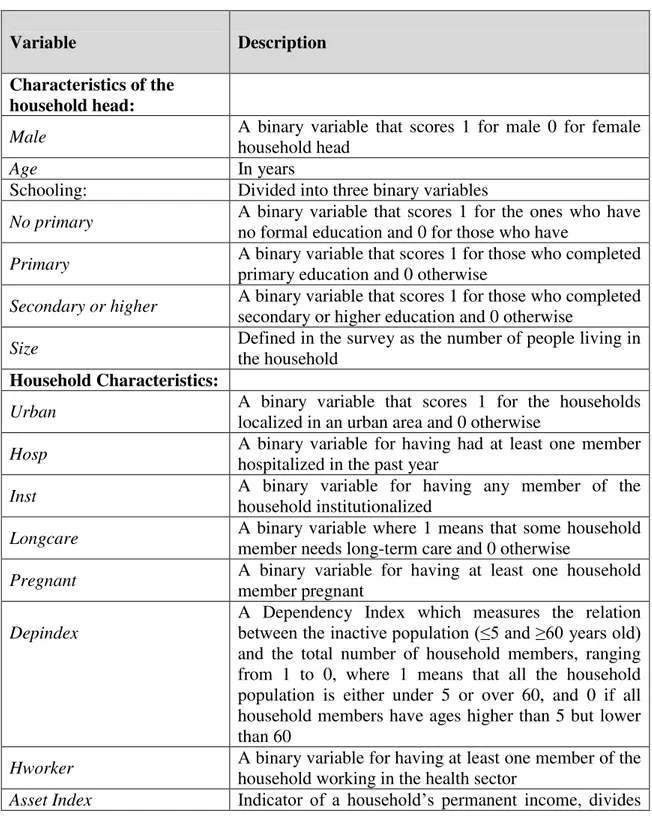
To explain the coping strategies adopted and to identify particular population groups associated with larger health expenditures, several factors are considered, described in the following table.
Table 3. Definition of variables:
Variable Description
Characteristics of the household head:
Male A binary variable that scores 1 for male 0 for female
household head
Age In years
Schooling: Divided into three binary variables
No primary A binary variable that scores 1 for the ones who have
no formal education and 0 for those who have
Primary A binary variable that scores 1 for those who completed
primary education and 0 otherwise
Secondary or higher A binary variable that scores 1 for those who completed
secondary or higher education and 0 otherwise
Size Defined in the survey as the number of people living in
the household
Household Characteristics:
Urban A binary variable that scores 1 for the households
localized in an urban area and 0 otherwise
Hosp A binary variable for having had at least one member
hospitalized in the past year
Inst A binary variable for having any member of the
household institutionalized
Longcare A binary variable where 1 means that some household
member needs long-term care and 0 otherwise
Pregnant A binary variable for having at least one household
member pregnant
Depindex
A Dependency Index which measures the relation between the inactive population (≤5 and ≥60 years old) and the total number of household members, ranging from 1 to 0, where 1 means that all the household population is either under 5 or over 60, and 0 if all household members have ages higher than 5 but lower than 60
Hworker A binary variable for having at least one member of the
household working in the health sector
the households into quintiles
Quintiles
Five quintiles in the form of binary variables that score 1 if the household belongs to that quintile and 0 otherwise
Country dummies Thirteen binary variables that score 1 if the household
belongs to that country and 0 otherwise
Since information about the household‟s income was not given by the survey
and to allow for further comparisons within countries, an Asset Index was used as
indicator of a household‟s permanent income. A total of 25 dummies containing the
assets that the households owns were used. Such index was calculated for each household using a weighted index calculated through principal components analysis (PCA). PCA is an exploratory multivariate statistical technique for simplifying complex datasets. The defining characteristic of PCA is that it assumes that all of the variability in an item should be used in the analysis. Given m (different from country to country) observations on 25 variables, the goal of PCA is to reduce the dimensionality of the data matrix by finding r new variables, where r is less than 25. Termed principal components, these new r variables together account for as much of the variance in the original 25 variables as possible while remaining mutually uncorrelated and orthogonal. Each principal component is a linear combination of the original variables, such that researchers often ascribe meaning to what the variables represent. PCA has been applied to asset questions in household surveys under the assumption that it is long-run wealth or permanent income that is the phenomenon attributable to the linear index of variables with the largest amount of information common to all of the variables (Ferguson et al., 2003). The result of such application of PCA is an asset index for each household according to the formula:
where is the scoring factor for the first asset as determined by the procedure, is the i-th household‟s value for the first asset and and are the mean and standard deviation of the first asset variable over all households. The index was then divided into equal quintiles. And five binary variables were constructed scoring 1 if the household‟s asset index result is from that particular quintile and 0 otherwise.
3.5 Regression Models
The regression models used include the regular probit model, an ordered probit and a tobit model. For the strategies estimation, firstly, an ordered probit model was estimated. The dependent variable is a latent variable illustrating the financial hardship imposed by the existence of health expenditures, penalization. This model additionally gives us the probability of using one of the strategies described before.
Secondly, three probit models were estimated separately for the probability of using the strategies households have available to cope with health expenditures: own resources; selling assets; and borrowing from family and others outside the household.
For the estimation of expenditures, first, a probit model was estimated for the factors that influence the probability of having health expenditures. And finally, a tobit model was estimated to evaluate the linear relationship between variables when there is a left-censoring (having expenditures higher than 0) in the dependent variable HE2.
keeping all the other covariates constant. This analysis is conducted when in the presence of a latent dependent variable.
The models were run separately for each of the thirteen countries using the same set of independent variables and together including specific dummies for the countries.
The reference category for education is no primary, the reference category for the asset index is the first quintile and the reference category for the countries dummies is country 1 (Burkina Faso).
Section 4. Results
The models were run first country-by-country and then to the full sample of countries. Including in the second case a dummy variable for each country.
4.1 The choice of coping strategies
Table A38 reports the ordered probit estimated for the penalization index. We first report on the country-by-country estimates.
The factors that influence significantly penalization of household resources are: a greater size of the household (for 6 countries) and having hospitalized members (for 7 countries) increase the penalization of households‟ resources, while being
localized in an urban area decreases the penalization (for 8 countries).
Other factors influence significantly, positive and negatively the penalization of resources, but in a smaller number of countries. Factors that also increase penalization are increasing age, having members who need long-term care, having
8
pregnant women in the household, and being in quintile 2. Factors that decrease penalization include having a male household head, a greater dependency index and being in quintile 3 and 4. The rest of the variables increase significantly the dependent variable in some countries and decrease in others.
By regressing the model with the full sample of countries together (Table A4, page 33), allowing for country-specific effects, penalization of resources seem to be significantly increased by a higher age of the household head, greater household size, having hospitalized and institutionalized members or even members who need long-term care, as well as having members working in the health sector. On the other hand, penalization is significantly decreased by having a household head who completed primary and secondary or a higher educational level, by households localized in an urban area, by a higher dependency index and being in the 5th quintile. Analysing the quintiles coefficients, they clearly illustrate the common belief that households at a lower quintile are subject to a higher penalization and this effect would decrease across quintiles. That is, families at the lowest quintiles have to use penalizing strategies.
4.2 Individual strategy choice
Table A59 reports the results of the estimated probit for the first strategy analyzed, use of own resources.
Having a male household head (for 5 countries) and that completed secondary or a higher educational level (for 4 countries) increases the probability of using income and savings to cope with health expenditures, as well as having a greater household size (for 5 countries) or a household localized in an urban area (for 6 countries). While having hospitalized members (for 5 countries) in the household decreases the probability of using income and savings. This effect enlighten us about the higher costs of hospitalization to the households.
Table A610 reports the results of the estimated probit for the second strategy, selling assets. The vulnerability of the households to the use of this strategy increases with a greater household size (for 8 countries) and by having hospitalized members (for 7 countries), contrary to the precious strategy. Whereas living in an urban area (for 10 countries) and having a household head who completed secondary or a higher educational degree (for 7 countries) decreases the probability of selling assets to cope with the existence of health expenditures, which is consistent with the effect found on using own resources.
Table A711 reports the results of the estimated probit for the last strategy, borrow from family or others who do not belong to the household. Households exposed to the use of this strategy are characterized by a greater age of the household head (for 6 countries), having hospitalized members (for 9 countries) and female household head (for 7 countries).
9
See Table A5, page 34.
10
See Table A6, page 35.
11
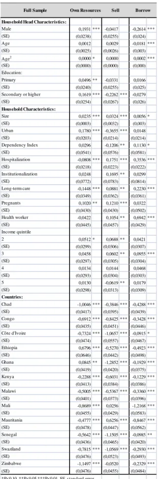
Table A812combines the results the probit models for the whole sample, including dummies for each country. The vulnerability of families towards using own resources, is increased by having a male household head, a household head who completed primary and secondary or a higher educational level, by a greater household size, by the location of the household being located in an urban area and in the 2nd quintile.
Additionally, households with a greater number of members use more the strategy of selling assets, as well as the ones having some of them hospitalized and institutionalized, members who need long-term care, pregnant women or even members who work in the health sector, as being in 2nd and 3rd quintiles. The probability of selling assets is on the other side decreased by having a household head who completed secondary or a higher degree of education, by a household localized in an urban area, a higher dependency index and being in the 5th quintile.
At last, the overall probability of borrowing to cope with health expenditures is decreased by having a male household head, although being increased by its age, the size of the household, the dependency index, having hospitalized members and who need long-term care, having members working in the health sector and by the household belonging to the 3rd quintile.
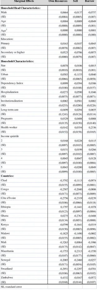
4.3 Marginal Effects13
In this sense, each set of dependent variables will be analyzed separately. Firstly, in terms of household-head characteristics being a male has the higher effect on the probability of using own resources, while its age has almost no impact. Secondly, in
12
See Table A8, page 37.
13
terms of broad household variables, being located in an urban area has a higher effect on the probability using own resources, while having some member who needs long-term care has the highest negative impact, followed by having an hospitalized member. Thirdly, in terms of quintiles distribution being at the first three quintiles has a higher impact on the probability of using own resources than being in the last two quintiles. Finally, in terms of countries, being in Ethiopia and Ghana increases slightly the probability of using own resources to cope with health expenditures, while for the rest of the countries the impact is negative and the highest in Zimbabwe.
In terms of marginal effects of the probability of selling assets to cope with health expenditures, in the household-head characteristics having completed secondary school or a higher educational level has the highest impact, while once again age has almost no effect. At the whole household level, having an hospitalized and institutionalizes member have the highest positive impact, a household located in an urban area seems to have the highest negative impact the probability of selling assets to cope with health expenditures. In terms of quintiles distribution being at the first three quintiles has a higher positive impact on the probability of selling assets than being in the last two quintiles. In fact, being at the 4th quintile has almost no effect and being at the 5th quintile decreases the probability of selling assets to cope with health expenditures In terms of countries, while being in Mali and Mauritania slightly increases the probability, for the rest of the countries the effect is negative, being the highest Ghana. Note that for the probability of using own resources living in Ghana actually had a positive impact.
household head characteristics. In terms of household variables, having some member who works in the health sector has the highest positive impact, followed by having an hospitalized member. Analyzing quintiles distribution being at the first four quintiles has a positive low effect on the probability of borrowing, being the highest impact of quintile 3, while being at the 5th quintile has almost no effect. Living in Mali decreases the probability of borrowing to cope with health expenditures, while for the rest of the countries the impact although negative is much lower.
4.4 Discussion
On the one hand, across countries we have a higher financial penalization on households with an older household head, illustrating the fact that when the household head attains a higher age threshold the household is more exposed to financial hardship. This effect can arise due to the fact that when the household head attains a certain age threshold, the contributions to the household income diminish, as does the disposable income to face health expenditures. A numerous family, as well as having members in a fragile health status (either hospitalized, institutionalized or in need for long-term care) contributes to the vulnerability of the household and puts them at risk of having to use more than their own resources to cope with health expenditures.
On the other hand, investing in education is proven to be beneficial for the probability of having to penalize the household resources, as well as living in an urban area, often more capable in terms of infrastructures to answer people‟s needs.
tend to find selling assets a less preferable strategy. Living in an urban area makes it difficult to sell assets what contradicts the intuition that in the face of a broad market selling assets would be a valuable strategy. A possible reason remains in the fact that households still have sufficient income and savings and so a lower probability of selling assets to cope with health expenditures. Can also be the case that the nature of assets in urban and rural areas is different, being easier to sell live stock for instance than a house or a car.
Additionally, having a bigger family indicates a higher probability of selling assets as a strategy to cope with health expenditures. A family with more members could mean less assets to sell, indicating that the marginal cost of selling an asset is lower than in the case of a larger family.
All in all, borrowing seems to be the more penalizing strategy for the overall sample of households.
Section 5. Determinants of Health Expenditure
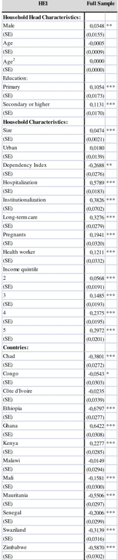
Table A1014 reports the probit model estimated for the probability of having Health Expenditures. In the majority of countries the probability of having health expenditures is positively influenced by the household head having a primary (for 6 countries) and secondary educational level (for 8 countries), the increase in the size of the household (all 13 countries), having hospitalized members (for 11 countries), those who need long-term care (for 11 countries) and pregnant women (for 6 countries) and being in the 3rd (for 7 countries), 4th (for 8 countries) and 5th (for 8 countries) quintiles.
14
The overall probability15 of having health expenditures is significantly increased by all variables, except for age, urban and dependency index. The latter significantly decreases the probability of having health expenditures.
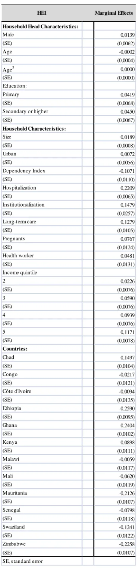
To evaluate the effect and the strength of the coefficients on the probability of having health expenditures we use marginal effects16, mentioned earlier in this section.
Firstly, in terms of household head characteristics completing primary and secondary or a higher educational degree has the highest impact on the probability having health expenditures. Secondly, a higher dependency index, that is, having a higher number of dependent members, strongly decreases the probability having health expenditures, while having an hospitalized member increases it. Thirdly, along the quintiles the impact on the probability of having health expenditures increases. And finally, in terms of countries, living in Ghana and Kenya increases the probability of having health expenditures, while for the rest of the countries the impact is negative and the highest for Ethiopia.
Table A1317 reports the tobit model results. The probability of having health expenditures greater than 018 is positively influenced by the household head having a primary (for 7 countries) and secondary educational level (for 8 countries), the increase in the size of the household (for 13 countries), the household being localized in an urban area (for 6 countries), having hospitalized (for 12 countries) and institutionalized members (for 9 countries), those who need long-term care (for 8 countries) and being in the 4th (for 8 countries) and 5th (for 10 countries) quintiles.
15
See Table A11, page 40.
16
See Table A12, page 41.
17
See Table A13, page 42.
18
Section 6. Concluding remarks
The vulnerability of families was found to be reflected mainly by their size, educational level and members in a poor health status. Educational level of the household was proven to be a greater drive for incurring in health expenditures. This fact illustrates that a more educated household do not spare on the essential in terms of health care. Nevertheless, for all strategies households at the lowest quintiles tend exploit them while facing health expenditures than people in the highest quintiles..
The choice of coping strategies also depends on the ability of households to borrow and the availability of assets. The former is linked not only to the financial capacity to repay a loan but also to the availability of social capital. The amounts needed may also differ from quintile to quintile. This could be a possible explanation to why there is no significant difference in the use of these coping strategies between lower quintiles in the majority of countries. Another reason is that the set of countries includes countries were the population is very poor and in that sense there is no large difference between the first quintiles.
Moreover, while we have searched for patterns in behavior among countries, it is also reasonable to believe that the precise mechanisms underlying coping strategies are likely to be context-specific both within and across countries. For instance, living in Mali was found to increase the vulnerability of a higher penalization of resources and in terms of individual strategies it had a positive impact in the probability of selling assets at the same time that decreases the probability of borrowing. For the majority of countries the effect in any choice of strategy is negative.
across time. In that sense, the study only captures the responses to an health shock in 2002 and not its consequences till today. Second, information on the amount of its own resources each household used, borrowed or the assets sold would be helpful for more perceptive analysis of the coping mechanisms used by households to finance health care.
References
Abel-Smith B, Rawal P. 1992. “Can the poor afford 'free' health services? A case study of Tanzania”, Health Policy Plan, Volume 7, Issue 4, pp. 329-341;
Banerjee. A, Duflo E. 2006. “The economic lives of the poor.”, Journal of
Economic Perspectives, Volume 21(1), pp. 141-167;
Ferguson. BD, Tandon A, Gakidou E, Murray CJL. 2003. “Estimating permanent income using indicator variables” [Evidence and Information
Policy Cluster Discussion Paper No.42]. Geneva: World Health Organization;
Flores. G, Krishnakumar J, O‟Donnell O, Van Doorslaer E. 2008. “Coping
with health care costs: implications for the measurement of catastrophic
expenditures and poverty”, Health Economics, Volume 17, pp.1393-1412;
Morduch. J. 1995. ”Income smoothing and consumption smoothing.”,
Journal of Economic Perspectives, Volume 9, pp.103-14;
Mwabu G, Mwanzia J, Liambila W. 1995. “User charges in government
health facilities in Kenya: effect on attendance and revenue.”, Health Policy Plan, Volume 10, Issue 2, pp. 164-170;
O'Donnell O, van Doorslaer E, Rannan-Eliya RP, Somanathan A, Adhikari SR, Akkazieva B, Harbianto D, Garg CC, Hanvoravongchai P, Herrin AN, Huq MN, Ibragimova S, Karan A, Kwon SM, Leung GM, Lu JF, Ohkusa Y, Pande BR, Racelis R, Tin K, Tisayaticom K, Trisnantoro L, Wan Q, Yang BM, Zhao Y. 2005. “Who pays for health care in Asia?”, Journal of Health Economics, Volume 27(2), pp.460-75;
Russell S. 2004. “The economic burden of illness for households in
and human immunodeficiency virus/acquired immunodeficiency syndrome.”, American Journal of Tropical Medicine and Hygiene, Volume 71, pp.147– 155;
Sauerborn. R, Adams A, Hien M. 1996. “Household strategies to cope with
the economic costs of illness.” Social Science & Medicine, Volume 43,
pp.291-301;
Russell. S. 1996. “Ability to pay for health care: concepts and evidence”,
Health Policy Plan; Volume 11, pp.219-37;
Wagstaff A. 2007. “The economic consequences of health shocks: evidence
from Vietnam 1993–98.”, Journal of Health Economics, Volume 26, pp.82– 100;
Wagstaff, A. and van Doorslaer, E. 2003. “Catastrophe and Impoverishment
in Paying for Health Care: with Applications to Vietnam 1993–98.” Health Economics, Volume 12(11), pp. 921–934;
Xu, K. 2005. “Distribution of Health Payments and Catastrophic
Expenditures. Methodology.” Geneva, WHO - Discussion paper No. 2.;
Xu. K, Evans DB, Kawabata K, Zeramdini R, Klavus J, Murray CJ. 2003. “Household catastrophic health expenditure: a multicountry analysis.” The Lancet, Volume 362, pp.111-117;
Xu. K, Evans D, Carrin G, Aguilar-Rivera AM, Musgrove P, Evans T. 2007. “Protecting households from catastrophic health spending.”, Health Affairs,
ANNEXES
Survey Questions
Section 0100. Sampling Information Q104. Setting:
1. Urban
2. Peri-urban/semi-urban
3. Rural
4. Other
Section 0400. Household Roster
C. Household member age
D. Household member education
Section 0500. Household Questionnaire
Q0500. Who is the person who provides the main economic support for the household?
Section 0560. Malaria Prevention: Use of (bed) nets
Q0563. Can you please tell me how many children aged under 5 years live in this household?
Q0565. Can you please tell me how many women who live in this household are currently pregnant?
Section 0570. Household Care
Q0570. Is there anyone in your house who is in an institution (hospital, after care home, home for the aged, hospice etc.) due to their health condition?
Q0571. Is there anyone in your home, a child or adult, who needs care because of a long-term physical or mental illness or disability, or is getting old and weak?
Section 0700. Permanent Income Indicators (Lower Income Countries) Q0700. Can you please tell me how many rooms there are in your home?
Q0701. How many chairs are there in your home?
Q0702. How many tables are there in your home?
Q0703. How many cars are there in your household?
Q0704. Does your home have electricity? Does anyone in your household have:
Q0704. A bicycle?
Q0706. A clock?
Q0707. A bucket?
Q0708. A washing machine for clothes?
Q0709. A washing machine for dishes?
Q0711. A fixed line telephone?
Q0712. A mobile / cellular telephone?
Q0713. A television?
Q0714. A computer ?
Section 0800. Household Expenditure
Q0804. Health care costs, excluding any insurance reimbursements
Q0815. In the last 12 months, how many times did members of your household go to a hospital and stay overnight?
In the last 12 months, which of the following financial sources did your household use to pay for any health expenditures?
Q0817 Current income of any household members
Q0818 Savings (e.g. bank account)
Q0820 Sold items (e.g. furniture, animals, jewellery, furniture)
Q0821 Family members or friends from outside the household
Q0822 Borrowed from someone other than a friend or family
Section 0900. Health Occupations
Q0900. Identification of member of the household who has ever worked or been trained in a Health-Related field.
Table A1. Insurance
Table A2. Descriptive Statistics
BurkinaChad Congo CdIvoireEthiopia Ghana Kenya Malawi Mali Mauritania Senegal Swaziland Zimbabwe
Insurance 6 0 553 0 4 90 37 1 0 18 13 27 361
Total 4745 4561 2924 3210 4987 3965 4326 5128 4862 3315 3323 2801 3982
% of Total 0 0 19 0 0 2 1 0 0 1 0 1 9
n= 4739 n= 4573 n= 2371 n= 3119 n= 4983 n= 3875 n= 4322 n= 5127 n= 4862 n= 3297 n= 3310 n= 2774 n= 3621
Household Head Characteristics: mean sd mean sd mean sd mean sd mean sd mean sd mean sd mean sd mean sd mean sd mean sd mean sd mean sd
Male 0,89 0,31 0,80 0,40 0,79 0,40 0,83 0,37 0,86 0,35 0,74 0,44 0,68 0,47 0,78 0,41 0,97 0,16 0,72 0,45 0,81 0,39 0,75 0,43 0,69 0,46 Age 42,37 16,24 40,59 16,88 40,89 14,46 41,18 15,30 42,31 16,09 43,47 17,47 39,66 17,80 37,18 16,82 53,11 15,96 42,91 17,28 48,78 15,85 42,97 17,00 39,05 18,35 Education:
No primary 0,84 0,36 0,82 0,39 0,24 0,43 0,53 0,50 0,63 0,48 0,50 0,50 0,42 0,49 0,67 0,47 0,91 0,29 0,70 0,46 0,67 0,47 0,44 0,50 0,30 0,46 Primary 0,08 0,27 0,10 0,29 0,29 0,45 0,21 0,40 0,00 0,00 0,35 0,48 0,26 0,44 0,22 0,42 0,05 0,21 0,13 0,34 0,17 0,37 0,24 0,43 0,38 0,48 Secondary or higher 0,08 0,27 0,09 0,28 0,47 0,50 0,27 0,44 0,37 0,48 0,15 0,36 0,31 0,46 0,10 0,31 0,05 0,21 0,17 0,38 0,16 0,37 0,31 0,46 0,33 0,47 Household Characteristics:
Size 5,81 3,14 5,09 2,92 5,06 2,89 5,31 3,36 5,58 2,37 5,21 2,92 4,27 2,54 4,38 2,25 8,91 3,61 5,75 2,80 7,97 3,41 5,56 3,19 4,97 2,40 Urban 0,41 0,49 0,24 0,43 0,82 0,38 0,61 0,49 0,15 0,36 0,39 0,49 0,32 0,47 0,16 0,36 0,25 0,43 0,43 0,50 0,48 0,50 0,24 0,43 0,32 0,47 Dependency Index 0,11 0,19 0,11 0,22 0,13 0,20 0,07 0,18 0,05 0,15 0,09 0,21 0,10 0,23 0,54 0,47 0,17 0,19 0,10 0,19 0,07 0,13 0,06 0,17 0,06 0,16 Hospitalization 0,15 0,35 0,11 0,31 0,15 0,35 0,13 0,34 0,04 0,20 0,21 0,41 0,15 0,35 0,20 0,40 0,08 0,27 0,21 0,41 0,13 0,33 0,08 0,28 0,11 0,31 Institutionalization 0,01 0,08 0,01 0,11 0,01 0,11 0,01 0,08 0,003 0,05 0,01 0,10 0,00 0,06 0,004 0,07 0,01 0,11 0,01 0,09 0,01 0,11 0,01 0,11 0,01 0,09 Long-term care 0,05 0,21 0,04 0,19 0,08 0,28 0,03 0,17 0,04 0,21 0,03 0,16 0,05 0,22 0,03 0,18 0,05 0,22 0,04 0,18 0,10 0,30 0,04 0,20 0,09 0,29 Pregnants 0,04 0,20 0,19 0,20 0,06 0,24 0,02 0,12 0,002 0,04 0,01 0,11 0,02 0,14 0,03 0,17 0,15 0,36 0,04 0,19 0,03 0,16 0,001 0,03 0,09 0,29 Health worker 0,11 0,31 0,01 0,09 0,05 0,21 0,02 0,14 0,01 0,09 0,02 0,15 0,03 0,16 0,02 0,16 0,04 0,19 0,01 0,11 0,04 0,19 0,04 0,20 0,00 0,06
Malawi Kenya
Ghana Mali Mauritania Senegal Swaziland Zimbabwe
32 3 . Or de re d p robit re sult s for the pe na li za ti on index :
Household Head Characteristics:
Male -0,0947 -0,2370* -0,0087 -0,1977 0,1890 -0,0129 -0,2132** 0,0167 -0,7010 0,1074 -0,2506* 0,0961 -0,1684
(SE) (0,0856) (0,1347) (0,1909) (0,1651) (0,1384) (0,1125) (0,0844) (0,1183) (1,0896) (0,1726) (0,1445) (0,1670) (0,1482)
Age -0,0438*** -0,0231 -0,0091 0,0331 -0,0153 -0,0006 0,0098 -0,0072 0,0688 0,0053 0,0194 -0,0272 -0,0201
(SE) (0,0091) (0,0142) (0,0269) (0,0230) (0,0134) (0,0107) (0,0097) (0,0136) (0,1213) (0,0205) (0,0175) (0,0194) (0,0181)
Age2 0,0005*** 0,0003** 0,0001 -0,0004 0,0002 0,0001 -0,0001 0,0002 -0,0006 0,0000 -0,0002 0,0004** 0,0003
(SE) (0,0001) (0,0002) (0,0003) (0,0003) (0,0001) (0,0001) (0,0001) (0,0002) (0,0011) (0,0002) (0,0002) (0,0002) (0,0002)
Education:
Primary -0,2029* 0,0650 -0,1299 -0,0267 d -0,0912 -0,0688 0,1039 0,0196 0,4969*** -0,3557** -0,0714 -0,0218
(SE) (0,1056) (0,1412) (0,1877) (0,1425) - (0,0876) (0,0866) (0,0857) (0,6418) (0,1820) (0,1533) (0,1512) (0,1714)
Secondary or higher -1,0045*** -0,2331 -0,1747 0,0634 -0,1740** -0,5384*** -0,3781*** 0,1559 -0,1524 0,5158*** -0,2113 -0,2110 -0,0871
(SE) (0,1401) (0,1542) (0,1847) (0,1302) (0,0808) (0,1466) (0,0876) (0,1144) (0,6480) (0,1678) (0,1488) (0,1566) (0,1814)
Household Characteristics:
Size 0,0350*** 0,0127 0,0296 0,0332** 0,0614*** 0,0249* 0,0634*** 0,0250 -0,0127 0,0545** 0,0022 0,0261 0,0227
(SE) (0,0096) (0,0166) (0,0245) (0,0161) (0,0173) (0,0137) (0,0139) (0,0170) (0,0031) (0,0224) (0,0149) (0,0219) (0,0256)
Urban -0,4693*** -0,5497*** 0,1578 0,1471 -0,6744*** -0,2912*** -0,6604*** -0,3993*** -1,5406*** 0,0700 -0,1761 -0,2396 -0,2913**
(SE) (0,0684) (0,1089) (0,2036) (0,1180) (0,1422) (0,0888) (0,0865) (0,1048) (0,4705) (0,1769) (0,1100) (0,1783) (0,1219)
Dependency Index -0,3102* -0,5276* -0,4003 0,4915 -0,5267 -0,4233 -0,1226 -0,2262 -0,4496 0,1762 0,1901 -0,4818 -0,0292
(SE) (0,1750) (0,2727) (0,4531) (0,3615) (0,4529) (0,2840) (0,2175) (0,2304) (1,3316) (0,4542) (0,4181) (0,7223) (0,5550)
Hospitalization 0,1253* 0,4784*** 0,7832*** 0,2027 0,6289*** 0,6578*** 0,4610*** 0,2140*** -0,5520 0,0651 0,1700 0,1690 -0,1133
(SE) (0,0723) (0,1015) (0,1653) (0,1317) (0,1194) (0,0871) (0,0869) (0,0768) (0,7668) (0,1498) (0,1206) (0,1595) (0,1360)
Institutionalization 0,3859 -1,0153* 1,2371*** 0,2254 0,4664 0,6318** -0,3643 0,0606 6,3892 -0,1371 0,1297 0,0566 -0,7413
(SE) (0,2644) (0,5680) (0,3852) (0,4307) (0,4412) (0,2703) (0,5728) (0,4712) (0,5288) (0,6181) (0,3719) (0,3591) (0,5531)
Long-term care 0,2480* 0,1765 -0,0667 -0,2311 0,0493 0,1508 0,5520*** 0,3420 -1,0202 0,2159 0,1053 0,1247 0,5011***
(SE) (0,1328) (0,2269) (0,2424) (0,2795) (0,1631) (0,2383) (0,1387) (0,1991) (0,8820) (0,2303) (0,1466) (0,2460) (0,1660)
Pregnants 0,0423 -0,1758 0,6137** -0,2041 -0,1884 -0,0882 -0,1245 0,1131 0,2349 0,0850 0,2402 d 1,1622
(SE) (0,1200) (0,1883) (0,2376) (0,3913) (0,6758) (0,3176) (0,2458) (0,1923) (0,5806) (0,2982) (0,2284) - (1,1017)
Health worker 10,4563 0,4159 -0,2966 0,0176 0,2066 -0,5891* -0,4887 0,8817*** -1,5816** 0,4563 -0,4102 0,2378 -0,5397*
(SE) (412.514) (0,3853) (0,3753) (0,4072) (0,5230) (0,3286) (0,3359) (0,1908) (0,6615) (0,3802) (0,2952) (0,2956) (0,3272)
Income quintile
2 0,0256 -0,0661 -0,2473 0,0928 -0,0368 0,0309 -0,0609 0,2133* -0,4784 0,7039 0,0870 -0,0616 0,2265
(SE) (0,0915) (0,1820) (0,2044) (0,1896) (0,1098) (0,1214) (0,1025) (0,1098) (0,8473) (0,4295) (0,1362) (0,2121) (0,1859)
3 0,0735 0,1105 -0,5168** 0,2666 -0,2141* 0,1657 -0,1393 0,0343 -1,5088** 0,6364 -0,1847 0,1719 0,0295
(SE) (0,0905) (0,1665) (0,2127) (0,1803) (0,1193) (0,1225) (0,1053) (0,1124) (0,7562) (0,4259) (0,1562) (0,2043) (0,1902)
4 -0,0599 0,1166 -0,6255* 0,0518 0,0087 0,0873 -0,2020** 0,0751 -1,4237 0,6769 -0,3771** 0,1616 -0,0242
(SE) (0,2150) (0,1646) (0,2206) (0,1871) (0,1171) (0,1223) (0,1047) (0,1145) (0,7935) (0,4285) (0,1634) (0,1891) (0,1887)
5 -0,3780*** -0,1115 -0,2829 0,0240 -0,0881 0,2554** -0,2687** 0,0723 -1,1617 0,8976** -0,2253 -0,0733 -0,1416
(SE) (0,1097) (0,1725) (0,2081) (0,1847) (0,1220) (0,1197) (0,1080) (0,1180) (0,6744) (0,4284) (0,1618) (0,1988) (0,1898)
*P<0.10, **P<0.05,***P<0.01, SE, standard error, d for dropped variable
Mauritania Senegal Swaziland Zimbabwe
Ethiopia Ghana Kenya Malawi Mali
Table A4. Ordered probit results for full sample:
Household Head Characteristics:
Male -0,0337
(SE) (0,0316)
Age -0,0087**
(SE) (0,0034)
Age2 0,0001***
(SE) (0,0000)
Education:
Primary -0,0567*
(SE) (0,0320)
Secondary or higher -0,1980***
(SE) (0,0322)
Household Characteristics:
Size 0,0336***
(SE) (0,0041)
Urban -0,3815***
(SE) (0,0271)
Dependency Index -0,2296***
(SE) (0,0776)
Hospitalization 0,2917
(SE) (0,0277)
Institutionalization 0,2214**
(SE) (0,1013)
Long-term care 0,2169***
(SE) (0,0475)
Pregnants 0,0539
(SE) (0,0614)
Health worker 0,6934***
(SE) (0,0559) Income quintile 2 0,0217 (SE) (0,0363) 3 -0,0153 (SE) (0,0364) 4 -0,0317 (SE) (0,0366)
5 -0,1246***
(SE) (0,0380)
Countries:
Chad -0,4537***
(SE) (0,0493)
Congo -1,0778***
(SE) (0,0693)
Côte d'Ivoire -1,2377***
(SE) (0,0581)
Ethiopia -0,7564***
(SE) (0,0453)
Ghana -1,3937***
(SE) (0,0455)
Kenya -0,8002***
(SE) (0,0434)
Malawi -0,9728***
(SE) (0,0443)
Mali 1,7992***
(SE) (0,1364)
Mauritania 0,5068***
(SE) (0,0446)
Senegal -1,1813***
(SE) (0,0533)
Swaziland -1,2219***
(SE) (0,0665)
Zimbabwe -0,4610***
(SE) (0,0634)
*P<0.10, **P<0.05,***P<0.01, SE, standard error
34 5 . P robit re sult s for own r esourc es stra te gy :
Household Head Characteristics:
Male 0,1389 -0,1791 ** 0,1059 0,1023 0,2345 0,3300 *** 0,3866 *** 0,2821 *** 0,0859 -0,1062 0,2688 *** 0,0742 0,1997**
(SE) (0,0902) (0,0894) (0,0944) (0,0946) (0,1884) (0,0700) (0,0633) (0,0758) (0,1919) (0,0987) (0,0873) (0,0902) (0,0976)
Age 0,0115 0,0153 * 0,0189 0,0185 * -0,3867 * -0,0015 -0,0023 0,0131 -0,0084 0,0081 -0,0030 -0,0136 0,0027
(SE) (0,0094) (0,0092) (0,0130) (0,0109) (0,0217) (0,0073) (0,0075) (0,0091) (0,0096) (0,0114) (0,0104) (0,0114) 0,0108
Age2 -0,0001 -0,0002 * -0,0002 * -0,0002 * 0,0004 * 0,0000 0,0000 -0,0002 * 0,0001 -0,0001 0,0000 0,0001 -0,0001
(SE) (0,0001) (0,0001) (0,0001) (0,0001) (0,0002) (0,0001) (0,0001) (0,0001) (0,0001) (0,0001) (0,0001) (0,0001) (0,0001)
Education:
Primary 0,3386 -0,0256 0,0512 0,1067 d -0,1037 0,0968 0,0751 *** 0,4262 *** 0,0379 0,1540 * 0,1253 -0,0061
(SE) (0,1059) (0,0943) (0,1017) (0,0827) - (0,0661) (0,7197) (0,0633) (0,1330) (0,1187) (0,0901) (0,0918) (0,1006)
Secondary or higher -0,1772 * 0,1814 * 0,0884 0,2070 ** -0,0307 0,0991 0,2702 *** 0,5454 0,1882 -0,0675 0,0324 0,0485 0,3012***
(SE) (0,1017) (0,1015) (0,1011) (0,0799) (0,1337) (0,0940) (0,0711) (0,1016) (0,1292) (0,1089) (0,0881) (0,0897) (0,1129)
Household Characteristics:
Size 0,0216 ** 0,0381 *** 0,0526 *** 0,0155 0,0008 0,0274 ** 0,0056 0,0114 0,0377 *** -0,0143 0,0160 0,0105 -0,0514***
(SE) (0,0109) (0,0113) (0,0130) (0,0099) (0,0268) (0,0110) (0,0115) (0,0122) (0,0079) (0,0139) (0,0098) (0,0123) (0,0163)
Urban -0,3866 *** 0,1778 ** 0,5616 *** 0,0192 0,0312 -0,0106 0,3845 *** 0,4510 *** 0,1922 *** 0,1027 0,0870 0,0292 0,6657***
(SE) (0,7409) (0,0724) (0,0958) (0,0686) (0,1805) (0,0625) (0,0673) (0,0826) (0,0651) (0,0139) (0,0687) (0,0958) (0,0823)
Dependency Index 0,2907 0,2798 0,0573 0,4536 * -0,5785 -0,3595 ** -0,0557 0,0542 0,1002 -0,1068 0,1888 -0,1641 -0,1226
(SE) (0,1985) (0,1741) (0,2026) (0,2365) (0,4927) (0,1644) (0,1561) (0,1600) (0,1505) (0,2375) (0,2899) (0,3635) (0,3353)
Hospitalization -0,0428 0,1572 ** -0,3514 *** 0,1362 * -0,3775 ** -0,4235 *** -0,1705 ** -0,0658 -0,1818 ** 0,0329 0,0590 0,1657 0,2761
(SE) (0,0749) (0,0727) (0,0882) (0,0825) (0,1726) (0,0661) (0,0712) (0,0584) (0,0794) (0,0924) (0,0834) (0,1018) (0,0921)
Institutionalization -0,0119 -0,5420 *** 0,1299 0,6067 d -0,4527 ** 0,0638 -0,0191 0,2260 0,7730 -0,0634 0,1704 0,4842
(SE) (0,2919) (0,1988) (0,2772) (0,4049) - (0,2172) (0,3912) (0,3368) (0,2139) (0,5122) (0,2558) (0,2604) (0,3428)
Long-term care -0,2891 ** -0,0967 -0,3928 *** 0,3182 * -0,4510 ** -0,1485 -0,0931 -0,2097 -0,0018 0,2186 -0,2024 ** 0,0993 -0,0412
(SE) (0,1171) (0,1539) (0,1139) (0,1744) (0,2107) (0,1545) (0,1092) (0,1356) (0,1068) (0,1717) (0,0932) (0,1581) (0,1096)
Pregnants 0,0326 0,1874 -0,1390 0,0495 d -0,1260 -0,0305 0,1258 0,0934 0,1299 0,0397 d -0,7096
(SE) (0,1467) (0,1371) (0,1396) (0,2374) - (0,2443) (0,1855) (0,1583) (0,0727) (0,2077) (0,1756) - (0,7261)
Health worker -0,2909 *** -0,0046 0,1417 -0,4555 ** d -0,2581 0,0076 -0,3284 ** 0,1152 -0,1280 -0,0953 -0,0076 0,5354**
(SE) (0,0860) (0,2818) (0,1636) (0,2119) - (0,1786) (0,1952) (0,1440) (0,1406) (0,3228) (0,1476) (0,1772) (0,2070)
Income quintile
2 0,6495 0,0840 0,0889 0,0552 -0,2328 -0,1319 -0,0457 0,0386 d 0,5009 *** -0,0043 0,0595 -0,0983
(SE) (0,1136) (0,1153) (0,1138) (0,1038) (0,2020) (0,0924) (0,0856) (0,0825) - (0,1366) (0,1006) (0,1162) (0,1197)
3 0,0854 0,2643 ** 0,1051 0,0329 -0,0168 -0,1262 -0,1084 0,0124 d 0,4885 *** -0,0541 0,1167 -0,0827
(SE) (0,1112) (0,1083) (0,1137) (0,1010) (0,2219) (0,0932) (0,0850) (0,0818) - (0,1324) (0,1053) (0,1191) (0,1207)
4 0,0578 0,1531 *** 0,0739 0,0319 -0,3336 0,0086 0,2918 -0,1438 * d 0,3244 ** -0,0846 0,2107 ** -0,0534
(SE) (0,1115) (0,1057) (0,1140) (0,1030) (0,2059) (0,0961) (0,0858) (0,0811) - (0,1368) (0,1034) (0,1122) (0,1201)
5 -0,0959 0,3861 -0,0229 0,1588 -0,1697 -0,2163 ** -0,0168 -0,1701 ** d 0,5747 *** -0,0608 0,3283 *** -0,0539
(SE) (0,1209) (0,1109) (0,1143) (0,1333) (0,2153) (0,0925) (0,0875) (0,0849) - (0,1452) (0,1065) (0,1135) (0,1196)
35 6 . P robit re sult s for selli ng a ssets st ra te g y :
Household Head Characteristics:
Male -0,0278 -0,1024 0,1187 -0,0886 0,1671 0,1200 -0,1144 * -0,0017 0,0529 -0,1153 0,0326 -0,0967 -0,2843***
(SE) (0,0798) (0,0924) (0,1359) (0,1144) (0,1331) (0,0906) (0,0664) (0,0794) (0,1914) (0,0967) (0,1160) (0,1140) (0,0963)
Age -0,0032 -0,0078 -0,0099 0,0378 ** -0,0005 -0,0020 0,0075 0,0047 -0,0075 0,0065 0,0059 -0,0090 0,0154
(SE) (0,0082) (0,0094) (0,0176) (0,0151) (0,0133) (0,0087) (0,0077) (0,0094) (0,0096) (0,0112) (0,0129) (0,0140) (0,0104)
Age2 0,0000 0,0001 0,0001 -0,0005 *** 0,0000 0,0001 0,0000 0,0000 0,0001 -0,0009 -0,0001 0,0002 -0,0002
(SE) (0,0001) (0,0001) (0,0002) (0,0002) (0,0001) (0,0001) (0,0001) (0,0001) (0,0001) (0,0001) (0,0001) (0,0002) (0,0001)
Education:
Primary -0,1931 ** -0,0327 0,1156 -0,0579 d -0,0730 -0,1463 ** 0,0955 0,2896 ** 0,0598 -0,5415 *** -0,1158 0,0565
(SE) (0,0934) (0,0984) (0,1336) (0,0958) - (0,0749) (0,0723) (0,0641) (0,1294) (0,1163) (0,1370) (0,1152) (0,0971)
Secondary or higher -0,8753 *** -0,2381 ** -0,2000 -0,2762 *** -0,1573 * -0,4372 *** -0,3481 *** -0,1015 0,1644 -0,0892 -0,2738 ** -0,0434 -0,1698
(SE) (0,1206) (0,1108) (0,1392) (0,0961) (0,0811) (0,1238) (0,0720) (0,0956) (0,1285) (0,1066) (0,1188) (0,1126) (0,1108)
Household Characteristics:
Size 0,0473 *** 0,1160 0,0248 0,0199 * 0,0698 *** 0,0219 * 0,0534 *** 0,0237 * 0,0416 *** -0,0145 0,0003 0,0209 0,0483***
(SE) (0,0092) (0,1173) (0,0175) (0,0115) (0,0172) (0,0119) (0,0114) (0,0123) (0,0079) (0,0136) (0,0122) (0,0152) (0,0159)
Urban -0,7820 *** -0,3558 *** -0,0428 -0,2737 *** -0,8855 *** -0,2899 *** -0,6929 *** -0,4174 *** 0,2024 *** 0,0804 -0,1841 ** -0,3264 ** -0,3379***
(SE) (0,0617) (0,0770) (0,1288) (0,0799) (0,1403) (0,0757) (0,0728) (0,0827) (0,0648) (0,0933) (0,0887) (0,1349) (0,0823)
Dependency Index -0,0070 -0,1304 0,0730 -0,1451 -0,2750 -0,3804 * -0,2934 * -0,2667 0,0794 -0,0916 0,2097 -0,5346 0,3551
(SE) (0,1655) (0,1801) (0,2870) (0,2946) (0,4142) (0,2229) (0,1665) (0,1639) (0,1504) (0,2347) (0,3457) (0,4853) (0,3321)
Hospitalization 0,0281 0,4131 *** 0,2354 ** -0,0951 0,5492 *** 0,4409 *** 0,3720 *** 0,1416 ** -0,1746 ** 0,0842 0,3345 *** 0,1740 0,0106
(SE) (0,0658) (0,0732) (0,1160) (0,0984) (0,1186) (0,0733) (0,0699) (0,0586) (0,0793) (0,0912) (0,0969) (0,1205) (0,0913)
Institutionalization 0,2253 -0,0377 0,7604 *** 0,0250 0,5301 0,3738 -0,3949 0,1215 0,2962 0,4741 -0,0234 0,0791 -0,4877
(SE) (0,2672) (0,1997) (0,2848) (0,3699) (0,4761) (0,2307) (0,4014) (0,3351) (0,2136) (0,4285) (0,3351) (0,2884) (0,3420)
Long-term care -0,0387 0,2456 -0,1191 0,1271 0,0108 0,3102 * 0,2344 ** -0,1069 -0,0262 0,2337 0,0735 0,1878 0,2580**
(SE) (0,1123) (0,1570) (0,1619) (0,1855) (0,1623) (0,1727) (0,1086) (0,1401) (0,1064) (0,1678) (0,1163) (0,1746) (0,1064)
Pregnants 0,1858 0,1470 0,5922 *** -0,2275 -0,4540 -0,0718 -0,0345 -0,0179 0,1158 -0,0373 0,2009 d -0,3594
(SE) (0,1209) (0,1394) (0,1648) (0,2906) (0,6269) (0,2812) (0,2024) (0,1545) (0,0725) (0,1964) (0,1888) - (0,6898)
Health worker 0,2219 *** 0,2998 -0,4100 -0,0204 -0,0710 -0,5840 ** -0,3305 0,7842 *** 0,1327 -0,1385 -0,4592 * 0,0417 -0,7826***
(SE) (0,0787) (0,2883) (0,2833) (0,2684) (0,5212) (0,2912) (0,2736) (0,1470) (0,1403) (0,3120) (0,2523) (0,2198) (0,2342)
Income quintile
2 0,0457 0,1028 -0,3218 ** -0,0155 -0,1223 0,1119 -0,0601 0,1386 d 0,4555 *** -0,0525 -0,1065 0,2117*
(SE) (0,0891) (0,1181) (0,1524) (0,1250) (0,1112) (0,1033) (0,0853) (0,0841) - (0,1348) (0,1118) (0,1448) (0,1165)
3 0,0978 0,1449 -0,2314 0,0982 -0,2684 ** 0,0747 -0,0946 0,0634 d 0,5346 *** -0,3069 ** 0,0296 0,2385**
(SE) (0,0880) (0,1114) (0,1487) (0,1194) (0,1201) (0,1069) (0,0856) (0,0842) - (0,1316) (0,1270) (0,1453) (0,1183)
4 -0,0316 0,1571 -0,4978 *** 0,1136 -0,0116 0,0034 -0,1879 ** 0,1803 ** d 0,3633 *** -0,4067 *** 0,0738 -0,0092
(SE) (0,0898) (0,1090) (0,1631) (0,1219) (0,1175) (0,1091) (0,0857) (0,0832) - (0,1357) (0,1294) (0,1353) (0,1178)
5 -0,2423 ** -0,0003 -0,2007 0,0592 -0,1031 0,2353 ** -0,2019 ** 0,1697 * d 0,5417 *** -0,3108 ** -0,1615 -0,0172
(SE) (0,1026) (0,1152) (0,1507) (0,1235) (0,1226) (0,1046) (0,0889) (0,0870) - (0,1429) (0,1310) (0,1440) (0,1179)
36 . P robit re sult s for the bor ro wing str ate gy :
Household Head Characteristics:
Male -0,0684 -0,4846 *** -0,2076 ** -0,4084 *** -0,2996 *** -0,5098 *** 0,2304 *** -0,3653 *** 0,4203 0,0820 -0,3853 *** -0,0100 -0,1259
(SE) (0,0910) (0,1029) (0,0976) (0,1019) (0,1304) (0,0636) (0,0619) (0,0804) (0,4345) (0,1364) (0,0882) (0,1017) (0,1019)
Age -0,0611 *** -0,0189 * -0,0158 -0,0303 *** -0,0095 -0,0171 *** -0,0023 -0,0237 ** 0,0035 0,0094 -0,0231 ** -0,0126 -0,0081
(SE) (0,0090) (0,0106) (0,0133) (0,0117) (0,0139) (0,0065) (0,0074) (0,0097) (0,0205) (0,0163) (0,0104) (0,0124) (0,0110)
Age2 0,0007 *** 0,0002 ** 0,0002 0,0004 *** 0,0001 0,0002 *** 0,0001 0,0003 *** 0,0000 -0,0001 0,0003 *** 0,0001 0,0001
(SE) (0,0001) (0,0001) (0,0001) (0,0001) (0,0001) (0,0001) (0,0001) (0,0001) (0,0002) (0,0002) (0,0001) (0,0001) (0,0001)
Education:
Primary 0,0078 0,1996 * -0,1260 0,1739 * d 0,0547 -0,1746 ** 0,0143 0,4542 ** 0,2245 -0,1499 0,1154 -0,0647
(SE) (0,1046) (0,1102) (0,1076) (0,0937) - (0,0594) (0,0702) (0,0705) (0,1921) (0,1495) (0,0921) (0,1013) (0,1041)
Secondary or higher -0,1001 0,1477 0,0649 0,1624 * -0,1266 -0,0744 -0,2480 *** 0,0676 0,0288 0,2848 ** -0,1050 -0,0177 -0,0688
(SE) (0,1118) (0,1217) (0,1054) (0,0909) (0,0970) (0,0823) (0,0679) (0,0992) (0,2418) (0,1362) (0,0910) (0,1017) (0,1180)
Household Characteristics:
Size -0,0081 0,0140 0,0303 ** 0,0179 -0,0075 0,0014 -0,0062 0,0073 -0,0096 0,0416 ** 0,0006 -0,0007 -0,0144
(SE) (0,0103) (0,0137) (0,0133) (0,0111) (0,0198) (0,0096) (0,0111) (0,0132) (0,0154) (0,0180) (0,0099) (0,0138) (0,0171)
Urban 0,2340 *** -0,1259 0,5792 *** -0,1006 0,4051 *** 0,0316 -0,1193 * -0,0497 -0,1798 0,1657 0,0268 -0,1734 -0,0628
(SE) (0,0706) (0,0896) (0,1112) (0,0778) (0,1216) (0,0556) (0,0622) (0,0840) 0,1300 (0,1381) (0,0699) 0,1105 (0,0887)
Dependency Index -0,3704 ** 0,0233 0,3281 -0,0876 -0,0931 0,2806 * 0,2455 0,1079 0,1528 0,0994 -0,0698 0,2387 0,4734
(SE) (0,1844) (0,2081) (0,2123) (0,2629) (0,4089) (0,1534) (0,1505) (0,1701) (0,2849) (0,3522) (0,2941) (0,3868) (0,3331)
Hospitalization 0,1317 * 0,6851 *** 0,7006 *** 0,3687 *** 0,6443 *** 0,7024 *** 0,4687 *** 0,2761 *** -0,0441 -0,0163 0,1108 0,2054 ** -0,0786
(SE) (0,0732) (0,0798) (0,0892) (0,0866) (0,1257) (0,0594) (0,0669) (0,0623) (0,1626) (0,1237) (0,0832) (0,1086) (0,0986)
Institutionalization 0,3680 -0,4316 * 0,4315 0,2391 -0,6232 0,1038 0,4579 -0,0748 -0,0796 -0,0201 -0,1093 -0,4000 -0,0841
(SE) (0,2523) (0,2444) (0,2686) (0,3267) (0,6286) (0,2177) (0,3600) (0,3736) (0,4367) (0,4806) (0,2688) (0,3143) (0,3610)
Long-term care 0,2821 ** 0,1623 -0,0847 0,0412 0,1532 0,3470 ** 0,3672 *** 0,4744 *** -0,0503 0,2054 0,0989 0,1272 0,3120***
(SE) (0,1217) (0,1816) (0,1202) (0,1757) (0,1699) (0,1449) (0,1038) (0,1350) (0,2150) (0,1959) (0,0953) (0,1697) (0,1109)
Pregnants -0,0678 -0,1524 0,2657 * 0,0682 0,5443 -0,1573 -0,0079 0,3463 ** -0,1385 0,2572 0,1869 d 0,0137
(SE) (0,1382) (0,1746) (0,1441) (0,2524) (0,5889) (0,2334) (0,1769) (0,1531) (0,1486) (0,2304) (0,1714) - (0,6995)
Health worker d 0,0539 0,1644 0,0111 0,3453 -0,4354 ** -0,4287 ** 0,4064 *** -0,4526 0,3944 -0,1628 0,0739 0,3911**
(SE) - (0,3281) (0,1603) (0,2526) (0,3678) (0,2000) (0,2012) (0,1522) (0,3104) (0,3220) (0,1571) (0,1992) (0,1952)
Income quintile
2 -0,0235 -0,0034 -0,0140 -0,0780 0,1458 0,1500 * -0,0801 -0,1057 2,5650 *** 0,2512 0,0324 0,0328 0,0242
(SE) (0,1026) (0,1483) (0,1189) (0,1178) (0,1356) (0,0833) (0,0822) (0,0918) (0,4183) (0,2175) (0,1024) (0,1296) (0,1241)
3 0,0192 0,2706 ** -0,1519 0,0314 -0,0927 0,3368 *** -0,0212 -0,0690 2,0621 *** 0,0400 0,1193 0,0541 0,0977
(SE) (0,1001) (0,1355) (0,1209) (0,1138) (0,1509) (0,0825) (0,0817) (0,0899) (0,3599) (0,2205) (0,1066) (0,1325) (0,1254)
4 -0,0837 0,2147 -0,2070 * -0,0968 0,1226 0,1711 ** -0,0636 -0,0161 1,7617 *** 0,0896 0,0526 -0,0194 -0,0536
(SE) (0,1037) (0,1334) (0,1209) (0,1181) (0,1446) (0,0840) (0,0811) (0,0895) (0,3632) (0,2238) (0,1052) (0,1258) (0,1262)
5 -0,2215 * 0,1598 -0,0420 -0,1629 0,1077 0,1671 ** -0,2131 ** -0,0264 1,8268 *** 0,3527 0,0246 -0,1460 -0,1435
(SE) (0,1164) (0,1398) (0,1189) (0,1181) (0,1479) (0,0848) (0,0847) (0,0926) (0,2873) (0,2225) (0,1088) (0,1292) (0,1272)