Experimental Investigations of the Existence of a Local-Time Effect on
the Laboratory Scale and the Heterogeneity of Space-Time
Victor A. Panchelyuga∗, Valeri A. Kolombet∗, Maria S. Panchelyuga∗and Simon E. Shnoll∗,†
∗Institute of Theor. and Experim. Biophysics, Russian Acad. of Sciences, Pushchino, Moscow Region, 142290, Russia †
Department of Physics, Moscow State University, Moscow 119992, Russia
Corresponding authors. Victor A. Panchelyuga: [email protected]; Simon E. Shnoll: [email protected]
The main subject of this work is an experimental investigation of the existence of a local-time effect on the laboratory scale, i.e. longitudinal distances between locations of measurements from one metre to tens of metres. A short review of our investigations of the existence of a local-time effect for longitudinal distances from 500 m to 15 km is also presented. Besides investigations of the minimal spatial scale for a local-time effect, the paper presents investigations of the effect in the time domain. In this relation the structure of intervals distribution in the neighbourhood of local-time peaks was studied and splitting of the peaks was revealed. Further investigations revealed second order splitting of local-time peaks. From this result it is concluded that space-time heterogeneity, which follows from the local-time effect, probably has fractal character. The results lead to the conclusion of sharp anisotropy of space-time.
1 Introduction
Our previous works [1–4] give a detailed description of mac-roscopic fluctuations phenomena, which consists of regular changes in the fine structure of histogram shapes built on the basis of short samples of time series of fluctuations in different process of any nature — from biochemical reactions and noises in gravitational antennae to fluctuations in α -decay rate. From the fact that fine structure of histograms, which is the main object of macroscopic fluctuation phenom-ena investigations, doesn’t depend on the qualitative nature of the fluctuating process, so it follows that the fine structure can be caused only by the common factor of space-time heterogeneity. Consequently, macroscopic fluctuation phe-nomena can be determined by gravitational interaction, or as shown in [5, 6], by gravitational wave influence.
The present work was carried out as further investiga-tions into macroscopic fluctuation phenomena. The local time effect, which is the main subject of this paper, is synch-ronous in the local time appearance of pairs of histograms with similar fine structure constructed on the basis of mea-surements of fluctuations in processes of different nature at different geographical locations. The effect illustrates the dependence of the fine structure of the histograms on the Earth’s rotation around its axis and around the Sun.
The local time effect is closely connected with space-time heterogeneity. In other words, this effect is possible only if the experimental setup consists of a pair of separated sources of fluctuations moving through heterogeneous space. It is obvious that for the case of homogeneous space the effect doesn’t exist. Existence of a local-time effect for some space-time scale can be considered as evidence of space-time heterogeneity, which corresponds to this scale. Dependence
of a local-time effect on the local time or longitudinal time difference between places of measurements leads to the con-clusion that space heterogeneity has axial symmetry.
The existence of a local time effect was studied for diffe-rent distances between places of measurement, from a hun-dred kilometres up to the largest distance possible on the Earth (∼15000 km). The goal of the present work is an inve-stigation of the existence of the effect for distances between places of measurements ranging from one metre up to tens of metres. Such distances we call “laboratory scale”.
2 Experimental investigations of the existence of a local-time effect for longitudinal distances between places of measurements from 500 m to 15 km
The main problem of experimental investigations of a local-time effect at small distances is resolution enhancement of the macroscopic fluctuations method, which is defined by histogram duration. All investigations of a local-time effect were carried out by usingα-decay rate fluctuations of239
Pu sources. Histogram durations in this case are one minute. But such sources of fluctuations become uselessness for distances in tens of kilometres or less when histogram durations must be about one second or less. For this reason in work [7–8] we rejectedα-decay sources of fluctuations and instead used as a source, noise generated by a semiconductor diode. Diodes give a noise signal with a frequency band of up to tens of megahertz and because of this satisfy the requirements of the present investigations.
work confirmed the suitability of diode semiconductor noise for studies of the local-time effect.
Below we present a short description of our experiments for investigation of a local-time effect for longitudinal dis-tances of 500 m up to 15 km between locations of measure-ments. The first experiment studied the local-time effect for a longitudinal distance of 15 km between locations of mea-surements, the second one for a set of longitudinal distances from 500 m to 6 km. A more detailed description of these experiments is given in [8].
In the first experiment a series of synchronous measure-ments were carried out in Pushchino (Lat. 54◦50.037′North, Lon. 37◦37.589′East) and Bolshevik (Lat. 54◦54.165′North, Lon. 37◦21.910′East). The longitudinal differenceαbetween places of measurements was α=15.679′. This value of α corresponds to a difference of local time ∆t=62.7 sec and longitudinal distance∆l=15 km.
To study the local-time effect in Pushchino and Bolshe-vik, we obtained 10-minute time series by digitizing fluc-tuations from noise generators with a sampling frequency of 44100 Hz. From this initial time series with three different steps of 735, 147 and 14 points, we extracted single mea-surements and obtained three time series with equivalent frequency equal 60 Hz, 300 Hz and 3150 Hz. On the basis of this time series, in a standard way [1–3] using a 60-point sample length for the first and second time series and a 63-point sample length for third time series, we constructed three sets consisting of histograms with duration 1 sec, 0.2 sec and 0.02 sec.
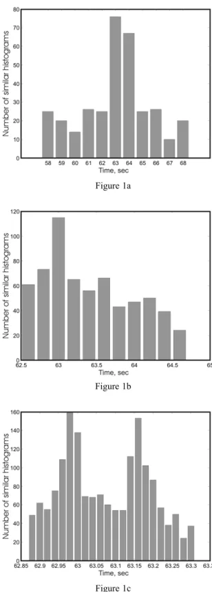
Fig. 1a depicts the intervals distribution obtained after comparisons of the 1-sec histogram sets. The distribution has a peak, which corresponds to a time interval of 63±1 sec, and which accurately corresponds to a local time difference
∆t=62.7 sec between places of measurements.
Local time peaks ordinarily obtained on the interval dis-tributions are very sharp and consist of 1–2 histograms [1–3] i.e. are practically structureless. The peak in Fig. 1a can also be considered as structureless. This leads us to the further investigation of its structure.
The fact that all sets of histograms were obtained on the basis of the same initial time series on the one hand, enables enhancement of time resolution of the method of investigation, and on the other hand, eliminates necessity of very precise and expensive synchronization of spaced measurements. The intervals distribution obtained for the 1-sec histograms set allows the use of information about the location of a local-time peak alignment of time series. The alignment makes possible the use of the set of histograms of the next order of smallness.
Using the 0.2-sec histograms set increased resolution five times and allowed more detailed investigations of local-time peak structure and its position on the local-time axis. Since the positions of the peak on the 1-sec intervals distribution (Fig. 1a) are known, it is possible to select their
neighbour-Figure 1a
Figure 1b
Figure 1c
hood by means of 60 sec relative shift of initial time series and prepare after this a 0.2-sec histograms set for further comparison.
The intervals distribution obtained from comparisons for the 0.2-sec histograms set is presented in Fig. 1b. One can see that maximum similarity of histogram shape occurs for pairs of histograms separated by an interval of 63±0.2 sec. This value is the same as for the 1-sec histogram intervals distribution, but in the latter case it is defined with an accu-racy of 0.2 sec.
It’s easy to see from the intervals distribution, Fig. 1b, that after fivefold enhancement of resolution, the distribution has a single sharp peak again. So a change of time scale in this case doesn’t lead to a change of intervals distribution. This means that we must enhance the time resolution yet again to study the local time peak structure. We can do this by using the 0.02-sec histograms set.
The intervals distribution for the case of 0.02-sec histo-grams is presented in Fig. 1c. Unlike the intervals distribu-tions in Fig. 1a and in Fig. 1b, distribution in Fig. 1c consists of two distinct peaks. The first peak corresponds to a local time difference of 62.98±0.02 sec, the second one to 63.16±
0.02 sec. The difference between the peaks is ∆t′=0.18± 0.02 sec.
Splitting of the local-time peak in Fig 1c is similar to splitting of the daily period in two peaks with periods equal to solar and sidereal days [9–11]. This result will be consi-dered in the next section.
The experiment described above demonstrates the exist-ence of a local-time effect for longitudinal distance between locations of measurements at 15 km, and splitting of the local-time peak corresponding to that distance. It is natural to inquire as to what is the minimum distance for the existence of a local time effect. The next step in this direction is the second experiment presented below.
In this experiment two measurement systems were used: stationary and mobile. Four series of measurements were carried out. The longitudinal differences of locations of stat-ionary and mobile measurement systems was 6 km, 3.9 km, 1.6 km and 500 m. The method of experimental data process-ing used was the same as for first experiment. It was found that for each of foregoing distances, a local-time effect exists and the local-time peak splitting can be observed.
3 Second-order splitting of the local-time peak. Preli-minary results
Four-minute splitting of the daily period of repetition of his-togram shape on solar and stellar sub-periods was reported in [3]. In that paper the phenomenon is considered as evidence of existence of two preferential directions: towards the Sun and towards the coelosphere. After a time interval of 1436 min the Earth makes one complete revolution and the measure-ment system plane has the same direction in space as one
stellar day before. After four minutes from this moment, the measurement system plane will be directed towards the Sun. This is the cause of a solar-day period — 1440 min.
Let us suppose that the splitting described in the present paper has the same nature as splitting of the daily period. Then from the daily period splitting ∆T=4 min it is pos-sible to obtain a constant of proportionalityk:
k= 240 sec
86400 sec ≈2.78
×10−3. (1)
The longitudinal difference between places of measure-ments presented in the second section is ∆t=62.7 sec and we can calculate splitting of the local-time peak for this value of∆t:
∆t′=k∆t=62.7×2.78×10−3≈0.17 sec. (2)
It is easy to see from Fig. 1c that splitting of the local-time peak is amounts to 0.18±0.02 sec. This value agrees with estimation (2). Values of splitting of the local-time peak, which were obtained for the mobile experiment, are also in good agreement with values obtained by the help of formula (2).
This result allows us to consider sub-peaks of local-time peak as stellar and solar and suppose that in this case the cause of splitting is the same as for daily-period splitting. But the question about local-time peak structure remains open.
In order to further investigations of the local-time peak structure an experiment was carried out using synchronous measurements in Rostov-on-Don (Lat. 47◦13.85′North, Lon. 39◦44.05′ East) and Bolshevik (Lat. 54◦54.16′ North, Lon. 37◦21.91′East). The local-time difference for these locations of measurements is∆t=568.56 sec. The value of the local-time peak splitting, according to (2), is∆t′=1.58 sec. The method of experimental data processing was the same as described in section 2.
In Fig. 2, a summation of all results of expert comparison is presented. For the considered case we omit presentation of our results in the form of interval distributions, like those in Fig 1, because it involves multiplicity graphs.
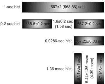
Fig. 2 consists of four lines. At the leftmost side of each line is the duration of a single histogram in the four sets of histograms, which were prepared for comparison. So we have four sets consisting of 1-sec, 0.2-sec, 0.0286-sec and 1.36 ms histograms. The rectangle in the first line schematically shows a local-time peak, obtained as a result of comparisons for the 1-sec histograms set. Taking into ac-count synchronization error (about one second), the result is 567±2 sec. This value is in agreement with the calculated lon-gitudinal difference of local time∆t=568.56 sec (through-out Fig. 2, calculated values are given in parentheses).
Fig. 2: Local-time peak splitting obtained in the experiment with synchronous measurements of fluctuations of a pair of semicon-ductor noise generators, carried out in Rostov-on-Don and Bol-shevik.
Fig. 3: Expected structure of local-time peak splitting for experi-ment with synchronous measureexperi-ments in Rostov-on-Don and Bol-shevik, calculated on the base of formula (4).
the rectangles gives the splitting of the local-time peak. The experimentally obtained splitting value is 1.6±0.2 sec, which is in good agreement with the value calculated on the basis of formula (2).
The third and fourth lines of Fig.2 present the results of additional investigations of local-time peak structure. In the third line is the result of comparisons of the 0.0286-sec histograms set for intervals, which constitute the closest neighbourhood of 567.2±0.2-sec peak. Using the 0.0286-sec histograms set increased resolution almost ten times and defines peak position on the intervals distribution at 567.22±
0.03 sec. The obtained peak is structureless. Further increase of resolution moves to the 1.36-ms histograms set, presented in fourth line. In this case resolution enhancement revealed splitting of 567.22±0.03 sec peak.
The splitting presented in last line of the diagram, can be regarded as second-order splitting. It can be calculated
using first-order splitting ∆t′
=1.58 sec by the analogue of formula (2):
∆t′′=k∆t′. (3) It easy to see from (3) and from Fig. 2, for second-order splitting∆t′′ the value of first-order splitting ∆t′ plays the same rˆole as the local-time value ∆t for ∆t′. Numerical calculations using (3) gives∆t′′=4.39 ms, which is in good agreement with the experimentally obtained splitting value 5.44±1.36 ms.
Experimental evidence for the existence of second-order splitting leads us to conjecture the possibility of n-order splitting. It easy to see from (2) and (3) that the n-order splitting value∆tncan be obtained in the following way:
∆tn
=kn
∆t . (4)
Fig. 3 presents an idealized structure of local-time peak splitting for the considered experiment, which was calculated on the base of formula (4). Unlike Fig. 2, the structure of local-time peak splitting in Fig. 3 is symmetrical. Studies of a possible splitting of 565.6±0.2 sec peak is our immediate task. At this time the results presented in the Fig. 2 can be considered as preliminary.
4 Experimental investigations of the existence of a local-time effect for longitudinal distances between places of measurements from 1 m to 12 m
The experiments described in two previous sections demon-strate the existence of a local-time effect for a longitudinal distance of 500 m between locations of measurements, and the existence of second-order splitting of the local-time peak. The next step in our investigations is a study of the local-time effect on the laboratory scale.
The main difference between local-time effect investiga-tions on the laboratory scale and the experiments described above is an absence of a special synchronization system. In the laboratory case the experimental setup consists of two synchronous data acquisition channels and two spaced noise generators, which are symmetrically connected to it. A LeCroy WJ322 digital storage oscilloscope was used for data acquisition. Standard record length of the oscilloscope consists of 500 kpts per channel. This allowed obtaining of two synchronous sets of 50-point histograms. The maximum length of every set is 10000 histograms.
Fig. 4 presents values of local time shift as a function of distance between two noise generators. The graph presents the results of investigations of a local-time effect for distan-ces of 1 m, 2 m, 3 m, and 12 m. Local-time values were found with an accuracy of 9.52 ms for the 12 m experiments and with an accuracy of 1.36 ms for the 1 m, 2 m, and 3 m experiments.
Fig. 4: Values of local time shift as a function of distance between two sources of fluctuations. The graph presents investigations of the local-time effect for distances 1 m, 2 m, 3 m, and 12 m.
Fig. 5. The intervals distribution was obtained on the basis of the 0.5-ms histograms set. Using the Earth’s equatorial radius value (6378245 m) and the latitude of the place of measurements (54◦50.0.37′), it is possible to estimate the local-time difference for a 1m longitudinal distance. The estimated value is 3.7 ms. It is easy to see from Fig. 5 that the experimentally obtained value of local-time peak is 4±0.5 ms, which is in good agreement with the theoretical value.
The results of our investigations for the laboratory scale, which are presented in this section, confirm a local-time effect for distances up to one metre. So we can state that a local-time effect exists for distances from one metre up to thousands of kilometers. This is equivalent to the statement that space heterogeneity can be observed down to the 1m scale.
5 Discussion
Local-time effect, as pointed out in [1], is linked to rotational motion of the Earth. The simplest explanation of this fact is that, due to the rotational motion of the Earth, after time
∆t, measurement system No. 2 appears in the same place where system No. 1 was before. The same places cause the same shape of fine structure of histograms. Actually such an explanation is not sufficient because of the orbital motion of the Earth, which noticeably exceeds axial rotational motion. Therefore measurement system No. 2 cannot appear in the same places where system No. 1 was. But if we consider two directions defined by the centre of the Earth and two points were we conduct spaced measurement, then after time
∆t measurement system No. 2 takes the same directions in space as system No. 1 before. From this it follows that similarity of histogram shapes is in some way connected
Fig. 5: Example of intervals distribution for longitudinal distance between two sources of fluctuations at one metre separation. Single histogram duration — 0.5 ms.
with the same space directions. This conclusion also agrees with experimental results presented in [12–13].
In speaking of preferential directions we implicitly sup-posed that the measurement system is directional and because of this can resolve these directions. Such a supposition is quite reasonable for the case of daily period splitting, but for splitting of the local-time peak observed on the 1m scale it becomes very problematic because an angle, which must be resolved by the measurement system, is negligible. It is most likely that in this case we are dealing with space-time structure, which are in some way connected with preferential directions towards the Sun and the coelosphere. Second-order splitting of local-time peaks can also be considered as an argument confirming this supposition. Apparently we can speak of a sharp anisotropy of near-earth space-time. Existence of a local-time effect leads us to conclude that this anisotropy is axially symmetric.
The Authors are grateful to Dr. Hartmut Muller, V. P. Ti-khonov and M. N. Kondrashova for valuable discussions and financial support. Special thanks go to our colleagues O. A. Mornev, R. V. Polozov, T. A. Zenchenko, K. I. Zenchen-ko and D. P. KharaZenchen-koz.
References
1. Shnoll S.E., Kolombet V.A., Pozharskii E.V., Zenchenko T.A., Zvereva I.M. and Konradov A.A. Realization of discrete states during fluctuations in macroscopic processes. Physics-Uspekhi, 1998, v. 41(10), 1025–1035.
3. Shnoll S.E. Periodical changes in the fine structure of statistic distributions in stochastic processes as a result of arithmetic and cosmophysical reasons.Time, Chaos, and Math. Problems, No. 3, University Publ. House, Moscow, 2004, 121–154.
4. Shnoll S.E. Changes in the fine structure of stochastic distri-butions as consequence of space-time fluctuations.Progress in Physics, 2006, v. 6, 39–45.
5. Panchelyuga V.A. and Shnoll S.E. Experimental investigations of gravitational-wave influence on the form of distribution function of alpha-decay rate. Abstracts of VI International Crimean Conference “Cosmos and Biosphere”, Partenit, Crimea, Ukraine, September 26 — October 1, 2005, 50–51.
6. Panchelyuga V.A. and Shnoll S.E. Experimental investigation of spinning massive body influence on fine structure of dis-tribution functions of alpha-decay rate fluctuations. In: Space-Time Structure, Moscow, TETRU, 2006, 328–343.
7. Panchelyuga V.A., Kolombet V.A., Kaminsky A.V., Panche-lyuga M.S. and Shnoll S.E. The local time effect observed in noise processes.Bull. of Kaluga University, 2006, No. 2, 3–8.
8. Panchelyuga V.A., Kolombet V.A., Panchelyuga M.S. and Shnoll S.E. Local-time effect on small space-time scale. In:
Space-Time Structure, Moscow, TETRU, 2006, 344–350.
9. Shnoll S.E. Discrete distribution patterns: arithmetic and cos-mophysical origins of their macroscopic fluctuations. Biophys-ics, 2001, v. 46(5), 733–741.
10. Shnoll S.E., Zenchenko K.I. and Udaltsova N.V. Cosmophys-ical Effects in the structure of daily and yearly periods of changes in the shape of histograms constructed from the mea-surements of 239Pu alpha-activity. Biophysics, 2004, v. 49, Suppl. 1, 155.
11. Shnoll S.E., Zenchenko K.I. and Udaltsova N.V. Cosmophys-ical effects in structure of the daily and yearly periods of change in the shape of the histograms constructed by results of measurements of alpha-activity Pu-239. arXiv: physics/ 0504092.
12. Shnoll S.E., Zenchenko K.I., Berulis I.I., Udaltsova N.V. and Rubinstein I.A. Fine structure of histograms of alpha-activity measurements depends on direction of alpha particles flow and the Earth rotation: experiments with collimators. arXiv: physics/0412007.