A new analytical inversion method for determining regional and global emissions of greenhouse gases: sensitivity studies and application to halocarbons

(1)

ACPD

8, 19063–19121, 2008

HFC inverse modeling

A. Stohl et al.

Title Page

Abstract Introduction

Conclusions References

Tables Figures

◭ ◮

Back Close

Full Screen / Esc

Printer-friendly Version

Interactive Discussion

Atmos. Chem. Phys. Discuss., 8, 19063–19121, 2008 www.atmos-chem-phys-discuss.net/8/19063/2008/ © Author(s) 2008. This work is distributed under the Creative Commons Attribution 3.0 License.

Atmospheric Chemistry and Physics Discussions

This discussion paper is/has been under review for the journalAtmospheric Chemistry

and Physics (ACP). Please refer to the corresponding final paper inACPif available.

A new analytical inversion method for

determining regional and global

emissions of greenhouse gases:

sensitivity studies and application to

halocarbons

A. Stohl1, P. Seibert2, J. Arduini3, S. Eckhardt1, P. Fraser4, B. R. Greally5, M. Maione3, S. O’Doherty5, R. G. Prinn6, S. Reimann7, T. Saito8,

N. Schmidbauer1, P. G. Simmonds5, M. K. Vollmer7, R. F. Weiss9, and

Y. Yokouchi8

1

Norwegian Institute for Air Research, Kjeller, Norway

2

Institute of Meteorology, University of Natural Resources and Applied Life Sciences, Vienna, Austria

3

University of Urbino, Urbino, Italy

4

(2)

ACPD

8, 19063–19121, 2008

A. Stohl et al.

Title Page

Tables Figures

◭ ◮

Back Close

Full Screen / Esc

5

School of Chemistry, University of Bristol, Bristol, UK

6

Center for Global Change Science, Massachusetts Institute of Technology, Cambridge, MA, USA

7

Swiss Federal Laboratories for Materials Testing and Research (Empa), Duebendorf, Switzerland

8

National Institute for Environmental Studies, Tsukuba, Japan

9

Scripps Institute of Oceanography, University of California, San Diego, CA, USA

Received: 5 September 2008 – Accepted: 25 September 2008 – Published: 13 November 2008

(3)

ACPD

8, 19063–19121, 2008

A. Stohl et al.

Title Page

Tables Figures

◭ ◮

Back Close

Full Screen / Esc

Abstract

A new analytical inversion method has been developed to determine the regional and global emissions of long-lived atmospheric trace gases. It exploits in situ measurement data from a global network and builds on backward simulations with a Lagrangian parti-cle dispersion model. The emission information is extracted from the observed

concen-5

tration increases over a baseline that is itself objectively determined by the inversion algorithm. The method was applied to two hydrofluorocarbons (HFC-134a, HFC-152a) and a hydrochlorofluorocarbon (HCFC-22) for the period January 2005 until March 2007. Detailed sensitivity studies with synthetic as well as with real measurement data were done to quantify the influence on the results of the a priori emissions and their

un-10

certainties as well as of the observation and model errors. It was found that the global a posteriori emissions of HFC-134a, HFC-152a and HCFC-22 all increased from 2005 to 2006. Large increases (21%, 16%, 18%, respectively) from 2005 to 2006 were found for China, whereas the emission changes in North America and Europe were modest. For Europe, the a posteriori emissions of HFC-134a and HFC-152a were slightly higher

15

than the a priori emissions reported to the United Nations Framework Convention on Climate Change (UNFCCC). For HCFC-22, the a posteriori emissions for Europe were substantially (by almost a factor 2) higher than the a priori emissions used, which were based on HCFC consumption data reported to the United Nations Environment Pro-gramme (UNEP). Combined with the reported strongly decreasing HCFC consumption

20

in Europe, this suggests a substantial time lag between the reported timing of the HCFC-22 consumption and the actual timing of the HCFC-22 emission. Conversely, in China where HCFC consumption is increasing rapidly according to the UNEP data, the a posteriori emissions are only about 40% of the a priori emissions. This reveals a substantial storage of HCFC-22 and potential for future emissions in China.

Deficien-25

(4)

ACPD

8, 19063–19121, 2008

A. Stohl et al.

Title Page

Tables Figures

◭ ◮

Back Close

Full Screen / Esc

or carbon dioxide are foreseen for the future.

1 Introduction

Over the past few decades, halocarbons have been used for refrigeration, as solvents, aerosol propellants, for foam blowing and for many other applications. Halocarbons containing chlorine and bromine lead to the depletion of ozone in the stratosphere

5

(Chipperfield and Fioletov, 2007) and, therefore, their usage has been regulated under the Montreal Protocol. As a consequence, chlorofluorocarbon (CFC) emissions have decreased considerably in recent years, but the emissions of hydrochlorofluorocarbons (HCFCs, used as interim replacement compounds for CFCs) are still growing in some countries. Hydrofluorocarbons (HFCs) are being used as replacement compounds for

10

most long-lived halocarbons containing chlorine and bromine and their emissions are increasing. Consequently, atmospheric concentrations of the more abundant HFCs (HFC-125, HFC-134a, HFC-152a) have been growing by about 10–14% per year (Forster et al., 2007b; Reimann et al., 2008; Greally et al., 2007; Clerbaux and Cunnold,

2007). While HFCs pose no danger for stratospheric ozone, they are e_ffective

green-15

house gases (GHGs). Thus, there is considerable interest in their emissions and they are included in the Kyoto Protocol Basket of GHGs whose emissions are regulated.

Halocarbon emissions can be determined using production, sales and consumption data such as provided by industry through the Alternative Fluorocarbons Environmen-tal Acceptability Study (AFEAS, 2007) (http://www.afeas.org/), by the Technology and

20

Economic Assessment Panel of the UNEP/IPCC (TEAP, 2005), or as reported in a number of other studies (e.g., McCulloch et al., 2003; Ashford et al., 2004b). The emis-sions can also be determined from atmospheric measurement data in conjunction with an atmospheric transport model that relates emissions to atmospheric concentrations, and an inversion algorithm. The inversion algorithm adjusts the emissions used in the

25

(5)

ACPD

8, 19063–19121, 2008

A. Stohl et al.

Title Page

Tables Figures

◭ ◮

Back Close

Full Screen / Esc

(1993) and Chen and Prinn (2006) used a global chemistry transport model and a linear Kalman filter, Mulquiney et al. (1998) a global Lagrangian model and a Kalman filter, Mahowald et al. (1997) a global chemistry transport model and a recursive weighted least-squares optimal estimation method. The spatial resolution at which source in-formation could be obtained with these global models was limited to the continental

5

scale. Furthermore, the halocarbon lifetimes are not known exactly, and this affects

the models’ capability to derive emission strengths. In fact, halocarbon lifetimes can be estimated using inverse models with prescribed emissions (Prinn et al., 2000).

Inverse methods have also been used to determine regional-scale halocarbon emis-sion fluxes. For instance, Manning et al. (2003) and O’Doherty et al. (2004) used data

10

from Mace Head, a Lagrangian particle dispersion model (LPDM), and a so-called simulated annealing technique to estimate halocarbon emissions over Europe. Even simple back trajectories combined with statistical methods have been used to derive halocarbon emission patterns qualitatively (Maione et al., 2008; Reimann et al., 2004, 2008). These methods have the advantage that they can assume that the halocarbons

15

are completely preserved over the short timescales (typically 4–10 d) considered and,

thus, are not a_ffected by uncertainties in a substance’s atmospheric lifetime. However,

they can only account for emissions that have occurred during the period of the cal-culation and leave a large fraction of the measured concentration unexplained. This so-called baseline, often said to be measured in air masses not recently perturbed by

20

emissions, must be subtracted from the measurements before the data can be used for the inversion. Unfortunately, the baseline is not clearly defined, especially in the Northern Hemisphere, and methods to determine it have all been subjective (see, e.g., Manning et al., 2003; Reimann et al., 2004; Maione et al., 2008). Furthermore, the inversion algorithms used on the regional scale (e.g. Manning et al., 2003; O’Doherty

25

(6)

ACPD

8, 19063–19121, 2008

A. Stohl et al.

Title Page

Tables Figures

◭ ◮

Back Close

Full Screen / Esc

solution in view of both the a priori emissions and the measured data.

An even simpler method of quantifying emission fluxes uses only measurement data. If the emissions of one chemical species with a lifetime longer than the duration of a typical transport event (e.g., carbon monoxide) are well known and those of another are reasonably well correlated with them ideally with co-located source, the unknown

emis-5

sions can be determined by the ratio of the measured concentration enhancements of the two species over their baseline (see Dunse et al., 2005; Yokouchi et al., 2006, for example). When combined with trajectory calculations, even regional quantification is possible to some extent.

In this paper, we develop a formal inversion method to determine the distribution of

10

HFC and HCFC sources. The advantages of our method are its analytical formulation which facilitates an e_fficient and accurate inversion, its capability of deriving both re-gional and global source strengths, the use of a priori information, and an appropriate treatment of uncertainties in the input data. The inversion builds on 20 d backward

simulations with a LPDM, which means that it is not a_ffected by uncertainties in the

15

halocarbon lifetimes. While a baseline must be determined, this is done in a way that is fully consistent with both the measurements and the model formulation. The uncer-tainty treatment also allows, for the first time in regional-scale inversions of halocarbon emissions, to use data from several stations concurrently. We apply the method here to HFC and HCFC emissions but it is suitable also for other long-lived trace gases.

20

We extensively test the new method at the example of the air-conditioning refriger-ant HFC-134a because of the large measurement data set available for this substance. The atmospheric abundance of HFC-134a, which has a lifetime of 14 years, is increas-ing at a rapid rate, in response to its growincreas-ing emissions arisincreas-ing from its role as a replacement for CFC refrigerants (McCulloch et al., 2003). We then apply the method

25

(7)

ACPD

8, 19063–19121, 2008

A. Stohl et al.

Title Page

Tables Figures

◭ ◮

Back Close

Full Screen / Esc

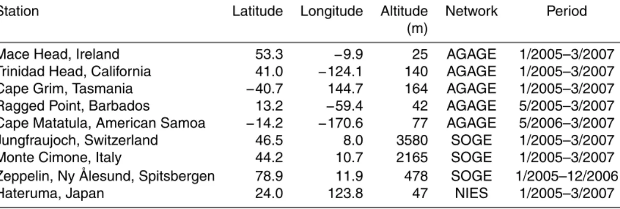
2 Measurement data

The HFC and HCFC data used in our inversions come from the three in situ at-mospheric measurement networks listed in Table 1: Advanced Global Atat-mospheric Gases Experiment (AGAGE) (Prinn et al., 2000); System for Observation of Halo-genated Greenhouse Gases in Europe (SOGE) (Greally et al., 2007); and Japanese

5

National Institute for Environmental Studies (NIES) (Yokouchi et al., 2006). Each of these networks uses automated low-temperature preconcentration and re-focussing to measure HFCs and HCFCs with an automated gas chromatograph/mass spectrometer (GC/MS). All the modelled data were averaged over 3-hourly intervals and paired with the corresponding 3-hourly model results for the respective measurement station. We

10

use data from January 2005 to March 2007.

At the five AGAGE stations, 2 l of ambient air are collected through stainless steel sampling lines and are analysed every two hours for about 40 analytes, including the HFCs and the HCFC modelled here, using a “Medusa” automated preconcentration and GC/MS instrument. The Medusa instrument employs two cryogenic traps to

pre-15

concentrate and refocus the 40 analytes from 2 l air samples prior to injection into the GC/MS, which is automated with custom control and data acquisition software. The Medusa instrument system, its operation and calibration procedures, and its perfor-mance, are described in detail by Miller et al. (2008).

At the SOGE stations Jungfraujoch and Ny- ˚Alesund, the ADS GC/MS system

devel-20

oped for AGAGE and described by Simmonds et al. (1995) and Reimann et al. (2004, 2008) is used. Every four hours, 18 halocarbons are analysed using 2 l of air. At the SOGE site of Monte Cimone a similar system as at Jungfraujoch and Zeppelin is in

op-eration (Maione et al., 2004, 2008). Di_fferences are that sampling is performed every

three hour with only 1 l of air. For all SOGE stations calibration is performed in a similar

25

way as for the Medusa system.

(8)

ACPD

8, 19063–19121, 2008

A. Stohl et al.

Title Page

Tables Figures

◭ ◮

Back Close

Full Screen / Esc

a stainless steel tube to the preconcentration system. Samples are analyzed once an hour, and after every five air analyses a gravimetrically prepared standard gas is analyzed for quantification.

Measurements of HFC-134a, HFC-152a and HCFC-22 in the AGAGE and SOGE networks are reported on the SIO-2005 primary calibration scale (Prinn et al., 2000;

5

Miller et al., 2008) through a series of comparisons between networks and should be directly comparable. However, the NIES data are independently calibrated using the Taiyo Nissan gravimetric scale. An intercomparison experiment for HFC-134a between NIES flask samples collected at Cape Grim and the AGAGE measurements at this sta-tion revealed that the NIES data are 1% too low compared to the AGAGE data. For

10

the inversions, we ignore this relatively small di_fference. Unfortunately, no

intercom-parisons have been made for HFC-152a and HCFC-22 but we assume them to be of a

similar magnitude as for HFC-134a. The implications of the different standards for the

inversions is that for Asia (which is constrained primarily by the Hateruma station), our

a posteriori HFC-134a emission fluxes will be biased low by<1% compared to other

re-15

gions, and the HFC-152a and HCFC-22 emissions have somewhat larger uncertainties than in other regions.

3 Model calculations

The inversion procedure is based on backward simulations with the Lagrangian particle dispersion model FLEXPART (Stohl et al., 1998, 2005, see also http://transport.nilu.no/

20

flexpart). FLEXPART was validated with data from continental-scale tracer experiments (Stohl et al., 1998) and has been used in a large number of studies on long-range atmo-spheric transport (e.g., Stohl et al., 2002, 2003, 2007; Damoah et al., 2004; Eckhardt et al., 2007). Here it was driven with operational analyses from the European Centre

for Medium-Range Weather Forecasts (ECMWF, 2002) with 1◦×1◦ resolution. In

ad-25

(9)

un-ACPD

8, 19063–19121, 2008

A. Stohl et al.

Title Page

Tables Figures

◭ ◮

Back Close

Full Screen / Esc

til January 2006; 91 vertical levels since then. No model calculations were made for February 2006 because of this discontinuity.

FLEXPART calculates the trajectories of tracer particles using the mean winds in-terpolated from the analysis fields plus random motions representing turbulence (Stohl and Thomson, 1999). For moist convective transport, FLEXPART uses the scheme

5

of Emanuel and ˇZivkovi´c-Rothman (1999), as implemented and tested in FLEXPART by Forster et al. (2007a). A special feature of FLEXPART is the possibility to run it backwards in time (Seibert and Frank, 2004). Such backward simulations from the measurement sites were made every 3 h. During every 3-h interval, 40 000 particles were released at the measurement point and followed backward in time for 20 d to

10

calculate an emission sensitivity, called source-receptor-relationship (SRR) by Seibert

and Frank (2004). The SRR value (in units of s kg−1_{) in a particular grid cell is}

pro-portional to the particle residence time in that cell and measures the simulated mixing ratio at the receptor that a source of unit strength (1 kg s−1) in the cell would produce. The SRR was calculated without considering removal processes. For HFC-152a, the

15

species with the shortest atmospheric lifetime considered in this paper (567 d), 3.5% would be lost after the maximum transport time of 20 d, which introduces a

system-atic underprediction of the emissions in the inversion of<3.5%. For the longer-lives

species HFC-134a and HCFC-22, this systematic error would be considerably smaller and, thus, we do not consider it further. Of particular interest is the SRR close to the

20

surface, as most emissions occur near the ground. Thus, we use SRR values for a so-called footprint layer 0–100 m above ground as the input to the inversion procedure. Folding (i.e., multiplying) the SRR footprint with the emission flux densities (in units of kg m−2s−1) (taken from an a priori emission inventory or from the inversion result) yields the geographical distribution of sources contributing to the simulated mixing ratio

25

at the receptor. Spatial integration of these source contributions gives the simulated mixing ratio at the receptor.

(10)

ACPD

8, 19063–19121, 2008

A. Stohl et al.

Title Page

Tables Figures

◭ ◮

Back Close

Full Screen / Esc

an average over the entire period investigated. There is a tendency of the network to sample ocean areas better than land areas on the 20 d time scale, which hampers the ability of the inversion method to determine emission source strengths over land. While some continents in the Northern Hemisphere (particularly Europe but also North America and large parts of Asia) are still quite well sampled, there are large regions

5

with very low sensitivity over tropical South America and Africa. Also India, Indonesia and northern Australia are not well covered. This means that emissions in these areas cannot be well determined with our method.

4 Inversion method

4.1 General theory

10

The estimation of gridded HFC emissions is based on the analytic inversion method of Seibert (2000, 2001). This method has recently been expanded by Eckhardt et al. (2008) to estimate the vertical distribution of sulfur dioxide emissions in a volcanic eruption column. They improved it to allow for an a priori for the unknown sources, a Bayesian formulation considering uncertainties for the a priori and the observations

15

and an iterative algorithm for ensuring a solution with only positive values. Here, the method is extended further considering a baseline in the observations which is adjusted as part of the inversion process, and more detailed quantification of errors. We repeat here the mathematical framework of the inversion, modified to include these extensions and adapted to other peculiarities of the problem.

20

We want to retrievenunknowns which are put into a vectorx, while themobserved

values are put into a vectoryo, where the superscriptostands for observations.

Mod-eled valuesy corresponding to the observations can be calculated as

y=Mx (1)

implying a linear relationship. Them×nmatrixMcontains the sensitivities of the

(11)

ACPD

8, 19063–19121, 2008

A. Stohl et al.

Title Page

Tables Figures

◭ ◮

Back Close

Full Screen / Esc

elled values y with respect to the unknowns x. The unknowns include the gridded

emission values as well as free parameters in the description of the baseline. The

sensitivity with respect to emissions is obtained from m FLEXPART backward

simu-lations, each with a transport time of 20 d. The transport model thus represents only concentration fluctuations caused by emissions during this time window of the air mass

5

history. Older emissions produce a background or baseline mixing ratio in the obser-vations to which the explicitly modelled part is added. As the emission sensitivity for

an age of>20 d is spread over large areas of the globe, the respective mixing ratio

contributions at a station vary rather smoothly with time. Therefore we describe them as a continuous, stepwise linear function with segments of 31 d length. The values at

10

then2nodes together with then1emission values are then=n1+n2unknowns. More

details are given later.

Typically, observations do not contain sufficient information to constrain well all ele-ments of the source vector, making the problem ill-conditioned. Therefore, regulariza-tion or, in other words, addiregulariza-tional informaregulariza-tion is necessary to obtain a meaningful

solu-15

tion. Often this additional information is provided in the form of a priori estimates of the unknowns. In combination with a quantification of the uncertainties of both unknowns and observations this leads to a Bayesian inversion minimizing a corresponding cost function.

If there is an a priori source vectorxa, we can write

20

M(x−xa)≈yo−Mxa (2)

and as an abbreviation

M ˜x≈y˜. (3)

Considering only the diagonals of the error covariance matrices (i.e., only standard deviations of the errors while assuming them to be uncorrelated), the cost function to

25

be minimized is

J=(M ˜x−y˜)T diag(σo

−2_{) (M ˜}

x−y˜)+x˜T diag(σx

−2₎ _˜

(12)

ACPD

8, 19063–19121, 2008

A. Stohl et al.

Title Page

Tables Figures

◭ ◮

Back Close

Full Screen / Esc

The first term on the right hand side of Eq. (4) measures the misfit model–observation,

and the second term measures the deviation from the a priori values. σo is the vector

of standard errors of the observations, andσx the vector of standard errors of the a

priori values. The operatordiag(a) yields a diagonal matrix with the elements of a in

the diagonal.

5

The above formulation implies normally distributed, uncorrelated errors, a condition that we know to be not fulfilled. Observation errors (also model errors are subsumed in this term) may be correlated with neighboring values, and deviations from the a priori sources are asymmetric. The justification for using this approach is the usual one: the problem becomes much easier to solve, detailed error statistics are unknown anyway,

10

and experience shows that reasonable results can be obtained. The implications of assuming normally distributed errors and how this limitation can be partly overcome follow later.

Minimization of J leads to a linear system of equations (LSE) to be solved for x˜

(Menke, 1984):

15

[MT diag(σo

−2_)]M

+diag(σx

−2_)] _˜

x=MT diag(σo

−2₎_˜

y (5)

The LSE is solved with the LAPACK1driver routine SGESVX, based on LU

factorisa-tion with calibrafactorisa-tion of rows and columns (if necessary) and iterative refinement of the solution.

Our algorithm presently does not yield an estimate of the uncertainty of x. This

20

desirable feature will be the subject of future development. However, already in its present development state, our algorithm is a substantial improvement over existing methods to determine regional halocarbon emission fluxes (e.g., Manning et al., 2003; Reimann et al., 2008), which do not consider uncertainties at all, also not in the input data.

25

1

(13)

ACPD

8, 19063–19121, 2008

A. Stohl et al.

Title Page

Tables Figures

◭ ◮

Back Close

Full Screen / Esc

4.2 Positive definiteness

Small negative “emissions” are not unrealistic in regions remote from industrial sources given that chemical and ocean sinks exist for halocarbons. These negative “emissions” are, however, negligible compared to the positive emissions on the time scale of 20 d

(<3.5% for HCFC-152a, the shortest-lived species considered). However,

inaccura-5

cies in model and data will in general cause our method to find solutions containing unrealistic negative emissions that are larger than expected. In the linear framework this cannot be prevented directly as positive definiteness is a nonlinear constraint. A workaround that has been adopted by Eckhardt et al. (2007) and which is also used here is to repeat the inversion after reducing the standard error values for those source

10

vector elements that are negative, thus binding the solution closer to the non-negative a priori values. This procedure is iterated until the sum of all negative emissions is less than 3‰ of the sum of the positive emissions. The standard errors are correspondingly recalculated in each step as

σ_xji =







0.5σ_xji−1 if x_ji−1<0 Min1.2σi−1

xj , σ 1 xj

if xi−1

j ≥0

(6)

15

wherexi−1

j andσ

i

xj denote thej-th elements of the source vector and of the vector of

uncertainties in the a priori source values, respectively, for thei-th iteration step.

4.3 The baseline definition

The substances studied here have lifetimes of the order of years. They are relatively well mixed in the troposphere and have a baseline upon which concentration variations

20

(14)

ACPD

8, 19063–19121, 2008

A. Stohl et al.

Title Page

Tables Figures

◭ ◮

Back Close

Full Screen / Esc

in order to use the inversion method. The baseline varies geographically and changes over time as the emission fluxes are not in equilibrium with the loss processes. In previous studies, various subjective combinations of data analysis and modeling were used to determine the baseline for individual stations (Manning et al., 2003; Greally et al., 2007). We aimed at a more objective method that can be applied equally for

5

all stations and that is consistent with our modeling approach. Thus, we define the baseline as that part of the measured concentration averaged over 31 d that cannot be explained by emissions occurring on the 20 d time scale of the model calculations.

Modelled concentrations are split into a part described by the transport simulation

y₁_l and the baseline party₂_l:

10

y_l =y₁_l +y₂_l =y₁_l+y_kb+_ttl −tk

k+1−tk

(y_kb₊₁−yb

k) (7)

whereldenotes a specific observation,k=1, . . . , n₂is the number of the corresponding

node and y_kb is the baseline value at node k (these values can be identified as the

baseline-related part of the vector of unknowns,x2). For an elementl of the modelled

time series, referring to a timetl,k refers to the node of the corresponding station and 15

the point in time wheret_k≤t_l<t_k₊₁.

The derivation of the sensitivies

m_kl = ∂y2l ∂x_k =

∂y2l

∂y_kb (8)

from Eq. (7) is trivial and corresponds to a linear interpolation between baseline values

at nodesk andk+1.

20

4.4 A priori baseline parameters and their uncertainty

For the practical application, xa, σx and σo need to be assigned proper values.

(15)

ACPD

8, 19063–19121, 2008

A. Stohl et al.

Title Page

Tables Figures

◭ ◮

Back Close

Full Screen / Esc

average measured mixing ratio minus the average a priori simulated mixing ratio dur-ing a 31 d interval. However, in order to reduce the dependence of the baseline on the a priori emissions, we filter out pollution events by excluding data above the me-dian of both the measured and the simulated values. Notice that for a polluted site with frequent contributions from recent emissions, the baseline defined in that way can

5

be below the lowest measured value, in contrast to previous methods (Manning et al., 2003; Greally et al., 2007). The uncertainty of the baseline values is taken to be 40% of the average a priori simulated emission contribution from the past 20 d, consistent with the assumed uncertainty for the emissions (see Sect. 4.5).

4.5 A priori emission data and their uncertainty

10

Regarding the a priori HFC-134a emissions (part ofxa), we took projections of global

total emissions from Ashford et al. (2004b) for the years from 2005–2007 and slightly adjusted them to make them fit with the AFEAS (2007) values for the year 2005 – the last year available with non-forecast data. When an inversion is done for a multi-year period, an average value weighted with the number of observations available for the

15

individual years is taken and the emissions are assumed to be constant.

For the spatial distribution of the emissions, we used total emissions for the year 2005 for countries where such information was available through the United Nations Frame-work Convention on Climate Change (UNFCCC, see http://unfccc.int). The country totals were disaggregated within each country’s borders according to a gridded

popu-20

lation density data set (CIESIN, 2005). We then subtracted the total UNFCCC emission

from the global total AFEAS emission and attributed the di_fference to all countries not

covered in the UNFCCC database, again distributing the emissions according to the CIESIN population. We also tested alternative disaggregation methods (see Sect. 5.2). Emission inventories tell us that HFC and HCFC emissions occur basically only over

25

(16)

ACPD

8, 19063–19121, 2008

A. Stohl et al.

Title Page

Tables Figures

◭ ◮

Back Close

Full Screen / Esc

The uncertainties of the emissions,σx, need to be specified for every grid cell.

Un-fortunately, no information on these uncertainties is actually available. Therefore, we have usedσ_xj=max(0.4xa_j , xa_{), where}_xa_{is the global average emission flux over the}

continents. The magnitude of these uncertainties was determined by trial and error, and was chosen to allow substantial corrections to the initial emission distribution.

5

4.6 Observation-related uncertainties

The vectorσoshould describe the part of the misfit between the observations and the

model results which is not due to wrong emissions. Thus it contains the measure-ment error as well as model errors. While information on measuremeasure-ment errors can be assessed from instrument characteristics, intercomparison tests etc., information

10

on model errors is difficult to obtain, though we assume that it is the dominant

con-tribution. Our first approach was to specify a σo for each individual station, as their

characteristics are quite di_fferent, but to assume it to be constant in time. It would be determined as the root mean square (RMS) error between a priori model output and observation, averaged for each station. Note that this is likely to be an overestimation.

15

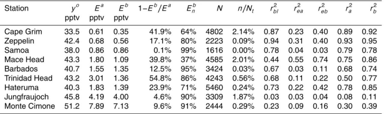
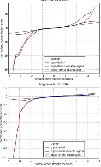
Investigating the resulting error statistics, both for the a priori and a posteriori results, we found that they are not normally distributed. This is mainly caused by a higher frequency of extreme values than expected for a normal distribution (i.e., a positive kurtosis excess), whereas the central part of the distribution is very close to normal (Fig. 2).

20

Another interesting feature is the amount of error reduction that is achieved in the inversion (Table 2). We see that for the two mountain stations, Jungfraujoch and Monte Cimone, the errors are much larger both before and after the inversion than for other stations. This is quite understandable as in mountain areas, processes are relevant for transport that cannot be resolved well, or not at all, by a global meteorological

25

(17)

ACPD

8, 19063–19121, 2008

A. Stohl et al.

Title Page

Tables Figures

◭ ◮

Back Close

Full Screen / Esc

events would be associated with underprediction by the model, and indeed as seen in Fig. 2 only the left tail is heavy at Jungfraujoch. These errors are “incurable” – the inversion cannot improve the agreement between the observations and the model results substantially. However, as the inversion minimizes quadratic errors, without additional measures taken they could have a disproportionately large influence on the

5

inversion result. As the theoretical approach implies normally distributed errors, the solution obtained is no more the most likely one in a Bayesian sense.

We tried to overcome this problem by assigning larger σo values to observations

causing very large errors. The kurtosisK of the error frequency distribution is used to

identify such large errors. For most stations,K is big if all errors are included.

There-10

fore, we sorted out the largest absolute errors step by step untilK of the remaining error values is below 5. The errors sorted out in this procedure were not entirely removed

from the inversion but their correspondingσ_ok were increased such that the frequency

distribution ofe_k/σ_ok(wheree_kare the individual errors) fits a normal distribution with a standard deviation taken from the central part of the error distribution. The standard

15

errors are first calculated using the a priori model results and are then re-calculated in three iteration steps using the a posteriori model results. The standard errors change only a little after the first iteration. Figure 2 shows the e_ffect of this normalization. At

Mace Head, the a priori error distribution is roughly Gaussian between values of −1

and+1.5 of the normal order statistic medians and this range is somewhat extended

20

by the inversion. However, there is a quite heavy tail on both ends. Our variable obser-vation error standard deviations are able to bring these tails quite close to the normal distribution after the inversion. At Jungfraujoch, we notice that positive errors (over-prediction) have a thin tail both before and after the inversion while the negative tail, indicating underprediction, is extremely heavy. Also here the variable weights bring the

25

left tail of the distribution much closer to normal.

The column with the normalized a posteriori errors (Enb) in Table 2 is the best

(18)

ACPD

8, 19063–19121, 2008

A. Stohl et al.

Title Page

Tables Figures

◭ ◮

Back Close

Full Screen / Esc

stations are not standing out anymore – an indication of the high observed variability there. By far the best performance is achieved at Mace Head with a relative error of 0.37. Cape Grim and Hateruma are the next best stations while the others have errors that are not much smaller than the observed variability.

4.7 Variable-resolution grid for the inversion

5

The size of the inversion problem is defined by the number of grid cells for which emission fluxes shall be determined. With a high-resolution global grid the problem

becomes quite big (e.g., 1◦×1◦corresponds to 64 800 unknowns). To reduce the

num-ber of unknowns, we use a variable-resolution grid with high resolution where such high resolution is warranted and lower resolution elsewhere. SRR values are high in

10

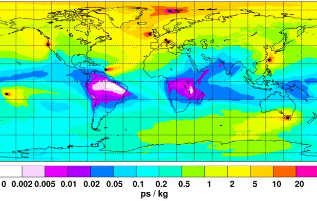
the vicinity of the observation sites but they decrease with distance from these sites (Fig. 1) lower resolution is su_fficient in these remote areas.

For setting up the variable-resolution grid, we start with a coarse 36◦

×36◦global grid,

whose resolution is enhanced in four steps to 12◦, 4◦, 2◦and 1◦, respectively. In every step, grid cells with a large total source contribution (the SRR field shown in Fig. 1

15

multiplied with the emission flux field) are subdivided, while grid cells with a low source contribution are kept at the coarse resolution. The fraction of boxes subdivided in an iteration step, here set to 50%, determines the total number of grid boxes used for the inversion. This creates a variable-resolution grid that has the highest resolution

(up to 1◦) in high-emission areas around the receptor sites, and the lowest resolution

20

(down to 36◦) in remote areas with low emission fluxes. An undesirable result of this

procedure is that coarse grid cells would be used wherever the a priori emission fluxes are very low, even in areas with large SRR values. To avoid this, a minimum emission flux (10% of the global mean) is used for calculating the source contribution values, thus enabling high resolution around the measurement stations even in areas where

25

(19)

ACPD

8, 19063–19121, 2008

A. Stohl et al.

Title Page

Tables Figures

◭ ◮

Back Close

Full Screen / Esc

5 Sensitivity studies

5.1 Idealized experiments

We tested our inversion method by determining the HFC-134a emissions in an ideal-ized set-up. For eight stations (Hateruma was removed to make Asia a region with poor data constraints) we fed the FLEXPART a priori model results plus baseline as pseudo

5

measurements into the inversion algorithm. In a first experiment, we used these data directly, in a second one we used them with superimposed noise. We then removed the a priori information by setting the emissions to zero everywhere, which is equiva-lent to a Tikhonov regularization (minimization of the total emission) to reconstruct the emission distribution. The number of pseudo observations available was 27 000, the

10

number of emission boxes 2800.

In the experiment without superimposed noise, the AFEAS/UNFCCC/CIESIN (AUC) emission field (Fig. 3a) is almost perfectly reconstructed by the inversion (Fig. 3b), with

small differences occurring mostly in Asia where there is a poor constraint by the

mea-surements. Consequently, the a posteriori modeled mixing ratios are virtually identical

15

to the pseudo measurements, as shown for Mace Head (Fig. 4a), which features a

Pearson correlation coefficient greater than 0.999. This shows that the inversion

al-gorithm has been set up correctly and is highly accurate. However, this experiment is not very realistic as the pseudo measurement data were constructed with the same transport model as was used for the inversion.

20

In the second experiment we mimicked measurement and model errors by superim-posing onto the pseudo measurements normally distributed random noise with

station-specific standard deviationσo(columnE

b

in Table 2). Even for this case, the emission distribution in Europe – the continent best constrained by the measurement data (see Fig. 1) – is very well reconstructed (Fig. 3c) and the total European emission is only

25

(20)

ACPD

8, 19063–19121, 2008

A. Stohl et al.

Title Page

Tables Figures

◭ ◮

Back Close

Full Screen / Esc

patterns and an overall underestimate of 50% (a result of the Tikhonov regularization constraining the emissions towards zero). A few “ghost” sources also appear at high northern latitudes, and emissions in the Southern Hemisphere (not shown), especially in Africa, are also not well reconstructed: continental totals are in error by more than a factor of 2. The pseudo measurements at the stations are well reproduced by the

5

inverse model, for instance at Mace Head (Fig. 4b), proving that it is the sparse density of measurement sites outside Europe that is most problematic for the inversion. An-other experiment showed that when pseudo measurements for the Hateruma station are added, the emission distribution in eastern Asia is well reconstructed.

5.2 Sensitivity to the a priori emissions and their assumed uncertainties

10

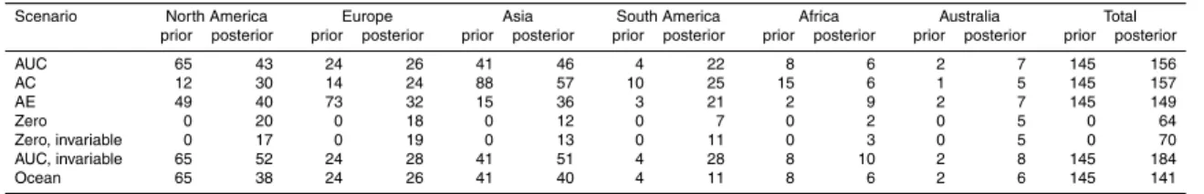
Next we evaluated the influence of the a priori emission information on the inversion for HFC-134a. All measurements from all stations (32 400 values in total) were used, and we studied the following five scenarios:

1. In our standard method, the CIESIN (2005) population map was used for distribut-ing the UNFCCC country emissions as well as the remaindistribut-ing AFEAS emissions

15

without country-specific information (AFEAS/UNFCCC/CIESIN or AUC).

2. The AFEAS global emissions were distributed only according to population with-out using UNFCCC information (AFEAS/CIESIN or AC).

3. The EDGAR version 3.3 inventory for the year 1995 (Olivier et al., 2001) was used for emission disaggregation (AFEAS/EDGAR or AE).

20

4. A zero emission flux was assumed everywhere (Tikhonov regularization, Zero).

5. Using the AUC a priori, we allowed the inversion to also produce non-zero emis-sion fluxes over the oceans (Ocean).

For the zero emission flux and the AUC inversion we also tested the influence of the assumed emission uncertainty. For that, we replaced our standard scenario (see

(21)

ACPD

8, 19063–19121, 2008

A. Stohl et al.

Title Page

Tables Figures

◭ ◮

Back Close

Full Screen / Esc

Sect. 4.5) with a globally constant uncertainty of 200% of the global mean emission flux.

The three a priori emission distributions (Fig. 5a, b; AC distribution not shown) are

quite different from each other. Continental total emissions as reported in Table 3 are

a factor of 7 and 6 higher in Africa and Asia for the AC distribution than for the AE

5

distribution. The AC distribution does not reflect different degrees of industrialization and likely overestimates emissions in less developed countries. Conversely, emissions in Europe are highest for the AE distribution, a result of the rather outdated EDGAR inventory for the year 1995 when HFC-134a emissions were still heavily weighted to-wards North America and Europe. The AUC distribution (Fig. 5a) lies between the AE

10

and AC distributions (Table 3) and is probably most realistic.

The a posteriori HFC-134a emissions (Fig. 5c, d, Table 3) differ much less than the

corresponding a priori emissions. Asian total emissions are more than doubled in the AE case, increased by 12% in the AUC case, and reduced by 35% in the AC case,

resulting in a maximum di_fference of 58% in the total a posteriori emissions, despite

15

the factor 6 difference in the a priori emissions. Emissions in China and Southeast

Asia, in particular, are increased substantially in the AE case.

Four stations located in Europe provide a strong constraint on European emissions.

The a posteriori total European emissions differ by a maximum of 33% (24–32 kt/yr,

see Table 3), although the AUC, AC and AE a priori emissions di_ffer by more than a

20

factor of 5. Also the resulting emission distributions within Europe are quite similar. The

weaker measurement constraint for North America results in slightly larger differences

between the a posteriori total emissions for that continent (43% di_fference compared

to more than a factor 5 in the a priori). Australian emissions, constrained mostly by the single station in Cape Grim, Tasmania are increased by approximately a factor of 4

25

over the a priori estimates. Possible reasons for this large discrepancy in the Southern Hemisphere are discussed below.

(22)

ACPD

8, 19063–19121, 2008

A. Stohl et al.

Title Page

Tables Figures

◭ ◮

Back Close

Full Screen / Esc

of the United States of America (USA), while increases occur in Canada and Alaska. Emission changes in Europe are spatially more complex, with a tendency of emission reductions in Central Europe and emission increases over the United Kingdom, Italy and Spain. In Asia, emissions are reduced by the inversion in India and southeast Asia but increased over China and Russia.

5

The zero a priori emissions scenario is particularly revealing, as it shows the capabil-ity of the method to identify emission areas without a priori information. Not surprisingly, the a posteriori emissions for this inversion are lower everywhere than when using non-zero a priori emissions (Table 3). However, the emission distribution in Europe is very well represented and total European emissions are only 30% lower than with the AUC

10

a priori distribution. Quite remarkably, also the strong emissions at the east coast of the USA are well reproduced, even though the constraint on these emissions mostly comes from the European stations (see Fig. 1). Australian emissions are also relatively well constrained and a strong emission source is also revealed in East Asia. Most en-couraging is the fact that the inversion does not produce artificial sources in regions

15

where strong emissions are unlikely.

For the zero a priori emission scenario, we also tested how strongly the inversion results depend on the assumed emission uncertainties. In our standard inversion, the uncertainty is 40% of the emission value in a grid box or 100% of the global mean emission flux, whichever is larger (for the zero a priori emission scenario, the AUC

20

uncertainties were used). As an alternative, we tested a spatially invariable uncertainty of 200% of the global mean emission flux (Fig. 5e). The continental total a posteriori values for the two uncertainty scenarios are almost identical (Table 3), except for South America where the masurement constraint is weak. The regional emission distribution within the continents is also similar for both scenarios but the patterns are smoother

25

when using the invariable emission uncertainty.

(23)

ACPD

8, 19063–19121, 2008

A. Stohl et al.

Title Page

Tables Figures

◭ ◮

Back Close

Full Screen / Esc

the source strengths in high-emission regions. In high-emission grid cells, the invari-able uncertainty is a too small fraction of the a priori source and, thus, the emissions are bound too tightly to their a priori values. The changes (a posteriori minus a priori) in the HFC-134a emission distribution are spatially more homogeneous when using the invariable emission uncertainty than when using a variable emission uncertainty

5

(Fig. 6). For instance, with the invariable uncertainty, emissions are reduced by the inversion almost all over the USA. In contrast, with the variable uncertainty, large re-ductions are made in at the east coast, with a more variable pattern of small increases and decreases elsewhere in the USA.

Our default setup ignores boxes where more than 99% of the area is covered by

10

water or ice. Allowing the inversion, using the AUC a priori emissions, to also produce emissions there, provides another check on the quality of the inversion. Although some spurious emissions can be found over the oceans in this case (Fig. 5f), their source strengths are all very low. In contrast, with the exception of South America which is poorly constrained by measurement data, the emissions over the continents remain

15

very similar to our default setup (Table 3).

5.3 Station-specific error statistics

Another way to look at the inversion results is to compare a priori and a posteriori errors at di_fferent stations for our default inversion using the AUC a priori (Table 2). At stations that are not too far from source regions (Cape Grim, Mace Head, Trinidad

20

Head, Hateruma) relative error reductions (1−Eb/Ea in Table 2) between 25% and

55% are achieved. At more remote stations such as Zeppelin and Barbados, errors are reduced by around 15%. At Samoa, the error reduction is marginal. This station is not influenced by sources on the time scale of 20 d included in our method (see Fig. 1); thus it cannot make a contribution to the inversion. The European mountain

25

(24)

ACPD

8, 19063–19121, 2008

A. Stohl et al.

Title Page

Tables Figures

◭ ◮

Back Close

Full Screen / Esc

have already been discussed in Sect. 4.6.

At most stations, the variability and trend in the baseline explains a substantial frac-tion of the observed HFC-134a variafrac-tions, shown as the squared Pearson correlafrac-tion coefficientr_bl2 between the a priori baseline and the observed concentrations in Table 2 (results using the a posteriori baseline are nearly identical). r_bl2 is highest for remote

5

stations (e.g.,r_bl2=0.94 for Zeppelin) where events with transport from source regions on the time scale of 20 d are rare, intermediate at stations not too far from source regions (e.g.,r_bl2=0.44 for Mace Head) where short-term variability is large, and low-est at the mountain stations where short-term variability dominates (e.g.,r_bl2=0.03 for Jungfraujoch).

10

Variability in the excess of the observed values over the baseline is mainly the result of transport events. A correlation analysis of the excess with the simulated emission contributions from the last 20 d reveals to what extent these events are captured by the

model. This was done using both the a priori (rea2 in Table 2) and a posteriori model

results (r_eb2 in Table 2). This analysis confirms the previous finding that the transport

15

model has no explanatory power at the remote station Samoa (r_eb2 =0.03). The model

also performs poorly at the mountain station Jungfraujoch (r_eb2 =0.04), partly because of some ”incurable” large errors, which were used with a reduced weight in the inversion but are included in the calculation of the correlation coe_fficients. The situation is a little better at the Monte Cimone mountain site (r_eb2 =0.16) where the inversion also results

20

in an improvement of the correlation. The model performs much better at the other sites. At Mace Head, it can even explain 74% of the observed short-term variance.

The correlations between observations and model results (i.e., baseline plus 20 d source contributions, r_a2 and r_b2 in Table 2) are high at all flatland stations (74–95% of the variance in the observations explained by the a posteriori model results). Only

25

at the mountain stations Jungfraujoch and Monte Cimone, the observations cannot be explained well (11–39%).

(25)

ACPD

8, 19063–19121, 2008

A. Stohl et al.

Title Page

Tables Figures

◭ ◮

Back Close

Full Screen / Esc

for the stations Mace Head and Trinidad Head where substantial error reductions could be achieved by the inversion. At both stations, the a priori concentrations are reduced, quite substantially so in the case of Trinidad Head where also the baseline is shifted upward to compensate for the reduced source contributions from the 20 d transport. At Mace Head, even the a priori simulation captures the majority of the transport episodes,

5

and the a posteriori results show excellent agreement with the measurements.

5.4 Tests with a subset of the data

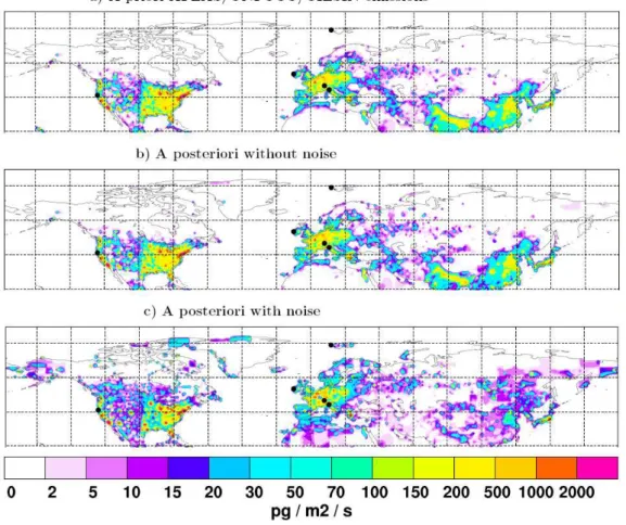
To investigate how sensitive the inversion result is to the availability of data from diff er-ent stations, we repeated the inversion using the AUC a priori information but in one case we removed all data from the Mace Head station and in another case we removed

10

all data from the mountain stations Jungfraujoch and Monte Cimone. The results are compared in Fig. 8 to the inversion using the full data set by showing the increments to the a priori caused by the inversion. Stations outside Europe were kept in the inversion but have a small influence on the results for Europe. The total European emissions are very similar in all three a posteriori cases (26.4, 28.0 and 24.4 kt/yr for the default

inver-15

sion, the case without Mace Head data and the case without Jungfraujoch and Monte Cimone data) and are all higher than in the a priori AUC inventory (24.2 kt/yr). This

shows that the measurement data from the di_fferent stations are quite consistent with

each other in constraining the European total emissions despite the modeling prob-lems at the mountain stations. A similar experiment done with the AE a priori, which

20

has a three times larger European total emission than the AUC a priori yielded similar a posteriori results, showing that the small di_fferences in the a posteriori total Euro-pean source strength is not the result of binding the inversions too tightly to the a priori. In fact, substantial corrections to the a priori occur on the regional scale. These

cor-rections are broadly consistent between the three di_fferent inversions shown in Fig. 8,

25

(26)

ACPD

8, 19063–19121, 2008

A. Stohl et al.

Title Page

Tables Figures

◭ ◮

Back Close

Full Screen / Esc

that even the data from the mountain stations are valuable in guiding the inversion on the regional scale. However, notice also that the removal of data from Mace Head has a stronger impact on the inversion than the removal of both Jungfraujoch and Monte Cimone data, a consequence of the lower model skill for the mountain stations. There are also some inconsistencies between the inversion results but they are mostly

re-5

stricted to individual grid boxes. For instance, emissions are increased over Madrid when Mace Head data are removed but decreased in the other cases, and the rel-atively large changes made to the emissions in Central Europe deviate somewhat in location between the di_fferent experiments.

Another inversion experiment was done using only data from Jungfraujoch, the

sta-10

tion with the poorest model performance. Also data from stations outside Europe were removed. The corrections to the a priori were much smaller in this case but the patterns were broadly consistent with the other results, showing for example emission increases in the United Kingdom and Eastern Europe.

In summary, our sensitivity experiments show that the inversion algorithm is working

15

properly as intended and produces consistent results both for idealized and realistic setups. In the following, we will apply the algorithm to determine the emissions of HFC-134a, HFC-152a and HCFC-22. While our inversion algorithm at present does not yield formal uncertainties of the a posteriori emission fluxes, we subjectively estimate that they are accurate to within better than 20% for Europe and to within 30% for other

20

(27)

ACPD

8, 19063–19121, 2008

A. Stohl et al.

Title Page

Tables Figures

◭ ◮

Back Close

Full Screen / Esc

6 HFC inversion results

6.1 HFC-134a

HFC-134a inversion results for our reference case using the AFEAS/UNFCCC/CIESIN a priori were presented in detail already in Sect. 5 and are further discussed here. To facilitate interpretation, we show results from inversions done separately for the years

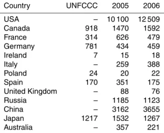
5

2005 and 2006, and we also report totals for some selected countries that are big enough to be resolved by our model grid. The results must be interpreted cautiously where large emissions occur near borders and, thus, attribution of the gridded emis-sions to a country is somewhat problematic (e.g., Canada, Germany). Both for the a priori as well as for the a posteriori results, total HFC-134a emissions increase from

10

2005 to 2006 (see Table 4). However, while the a priori emissions increase everywhere (no UNFCCC country-specific information was available for years after 2005 when this work was done), the a posteriori emissions increase in Europe (mostly in Eastern Eu-rope) and Asia (especially in China) but decrease in North America. The increase in Europe is a continuation of the upward trend seen also in the UNFCCC data until

15

2005, while the decrease in North America (due to a decrease in the USA, see Table 5) could indicate a trend reversal. UNFCCC data for the USA and Canada indeed show

a leveling-o_ffbetween 2004 and 2005 of the previously positive emission trend. Our a

posteriori emissions for the USA for 2005 (2006) are furthermore only 61% (50%) of the UNFCCC value.

20

For Europe, the a posteriori emissions are somewhat higher than the industry-based a priori emissions and suggest a 13% increase from 2005 to 2006. In con-trast, O’Doherty et al. (2004) found for several periods (latest period 2000–2002) that emissions derived from simulations with the NAME model and an inverse algorithm were about a factor 2 smaller than the industry-based value. If both model-derived

25

(28)

ACPD

8, 19063–19121, 2008

A. Stohl et al.

Title Page

Tables Figures

◭ ◮

Back Close

Full Screen / Esc

since their European emissions are only 12% of their reported global emissions, which seems low. Furthermore, Reimann et al. (2004) derived much higher European emis-sions of 23.6 kt/yr for the same period (2000–2002), almost identical to our estimate for 2005 and 2006. Still, our a posteriori source distribution in Europe is quite similar to that shown by O’Doherty et al. (2004), lending confidence to both approaches. The

5

source distribution is, however, very di_fferent from the potential source regions shown

by Reimann et al. (2008) and Maione et al. (2008) based on statistical analyses of back trajectories and HFC-134a data from the mountain sites Jungfraujoch and Monte Ci-mone. We attribute this to artifacts in their trajectory statistics, which are likely to occur especially in regions not frequently passed by trajectories.

10

While many western European countries (e.g., France, Ireland, Spain, United King-dom) had constant or slightly decreasing emissions from 2005 to 2006, emissions in some southern (e.g., Italy) and eastern (e.g., Poland) European countries increased (Table 5). In general, there is relatively good agreement between UNFCCC reported emissions and our a posteriori emissions for the year 2005 for most European

coun-15

tries.

For Asia, between 2005 and 2006 we find an increase of emissions in China and a decrease in Japan (Table 5). According to UNFCCC, emissions in Japan peaked in 2003 and decreased by 25% until 2005. Our results confirm decreasing emissions in Japan but the 2005 total is 50% higher than the UNFCCC total. For China, we obtain

20

annual emissions of 9.8 and 11.9 kt/yr for the years 2005 and 2006, respectively, sub-stantially more than the 3.9 kt/yr reported by Yokouchi et al. (2006) for the period May 2004 – May 2005, which was derived using Hateruma HFC-134a to carbon monoxide ratios and a – likely too low – estimate of Chinese carbon monoxide emissions. Our results indicate that China is now a substantial emitter of HFC-134a with a 20% growth

25

(29)

ACPD

8, 19063–19121, 2008

A. Stohl et al.

Title Page

Tables Figures

◭ ◮

Back Close

Full Screen / Esc

6.2 HFC-152a

HFC-152a has an estimated atmospheric lifetime of 1.55 yr (Greally et al., 2007) and is used predominately in foam-blowing and aerosol spray applications (Ashford et al.,

2004b). For HFC-152a, the a priori emission data were calculated slightly di_fferently

than for HFC-134a. As no global emission data from AFEAS are available, we used

5

projections from Ashford et al. (2004b) for 2005–2007 directly (i.e., without adjustment to AFEAS emissions). Furthermore, UNFCCC country total emissions are available for fewer countries than for HFC-134a. Where available, we used this information. Data for the USA – the largest emitter of HFC-152a, according to Ashford et al. (2004b) – are missing for confidentiality reasons. A distribution of emissions according to the

10

world population distribution would definitely lead to an underestimation of HFC-152a emissions in the USA (about 1 kt/yr). Inversion experiments done with such a low a priori value for the USA lead to a more than four-fold increase of emissions in the USA and unrealistically high emissions in border regions of Canada, as the inversion algorithm is trying to compensate for far too low USA emissions. To bring the a priori

15

estimate closer to the suspected real emissions, we therefore assumed an annual emission of 10 kt/yr in the USA, about 40% of the global emissions.

The inversion results in a substantial increase (55% for the whole period) of global HFC-152a emissions relative to the a priori emission from Ashford et al. (2004b) (see Table 4 and Fig. 9). The relative increase is larger for the full period than for the

20

individual years because the stronger constraint from the larger measurement data set can drive the a posteriori solution further away from the a priori emissions. This

e_ffect is especially evident in this case of HFC-152a where the a priori emissions are

systematically too low in all continents. Since the solution is bound towards a too low a priori, it is likely that our inversion results (particularly for the individual years) are

25

actually a lower estimate of the true global source strength.

(30)

ACPD

8, 19063–19121, 2008

A. Stohl et al.

Title Page

Tables Figures

◭ ◮

Back Close

Full Screen / Esc

HFC-152a emissions than reported by Ashford et al. (2004b) from industry data. For the year 2004, Greally et al. (2007) reported a source strength of 28.5 kt, compared to only 21.9 kt from Ashford et al. (2004b). Our results confirm this stronger source and also indicate that emissions have grown more rapidly from 2005 to 2006 than the industry-based estimate of Ashford et al. (2004b).

5

The inversion increases the emissions in all continents (see Table 4 and Fig. 9), even in North America, where high a priori emissions of 10 kt/yr for the USA alone were used. The smallest increases occur in Europe where many countries have reported their emissions to UNFCCC and our a priori estimate should be most accurate. Most of these increases occur in Southern Europe (see Fig. 9c), especially in Italy and in some

10

regions of Spain. European emissions derived by the inversion increased from 2005 to 2006, whereas emissions reported by the European Union decreased from 2003 to 2005. Increasing emissions higher than reported by the EU countries were already found by Greally et al. (2007) using inversions based on another LPDM and Reimann et al. (2004) using measurement data from Jungfraujoch. There is some agreement

15

in regional emission patterns in Europe between our results and those reported by Greally et al. (2007), Maione et al. (2008) and Reimann et al. (2008).

The inversion increases the emissions in Asia by about 50%, with a doubling of the a priori emissions in China (see Fig. 9) and a 16% increase from 2005 to 2006 (see Table 6). Our estimated Chinese HFC-152a emissions of 3.2–3.7 kt/yr are in good

20

agreement with the 4.3 kt/yr recently reported by Yokouchi et al. (2006) for the period May 2004 to May 2005.

HFC-152a emissions in Australia are relatively small (ca. 200–600 t/yr, depending on period) but significantly larger than the 5–10 t/yr reported by Greally et al. (2007). Figure 10 shows time series of 152a for the Cape Grim station in Tasmania.

HFC-25

152a concentrations are very low and the measurements show a lot of variability, which partly appear to be associated with instrumental noise and probably the advection of air masses with variable background but without recent emission input, which makes the