Correction method for line extraction in vision measurement.

(1)

Vision Measurement

Mingwei Shao, Zhenzhong Wei*, Mengjie Hu, Guangjun Zhang

Beihang University, Key Laboratory of Precision Opto-mechatronics Technology, Ministry of Education, Beijing, 100191, China

*[email protected]

Abstract

Over-exposure and perspective distortion are two of the main factors underlying inaccurate feature extraction. First, based on Steger’s method, we propose a method for correcting curvi-linear structures (lines) extracted from over-exposed images. A new line model based on the Gaussian line profile is developed, and its description in the scale space is provided. The line position is analytically determined by the zero crossing of its first-order derivative, and the bias due to convolution with the normal Gaussian kernel function is eliminated on the basis of the related description. The model considers over-exposure features and is capable of detect-ing the line position in an over-exposed image. Simulations and experiments show that the proposed method is not significantly affected by the exposure level and is suitable for correct-ing lines extracted from an over-exposed image. In our experiments, the corrected result is found to be more precise than the uncorrected result by around 45.5%. Second, we analyze perspective distortion, which is inevitable during line extraction owing to the projective camera model. The perspective distortion can be rectified on the basis of the bias introduced as a function of related parameters. The properties of the proposed model and its application to vi-sion measurement are discussed. In practice, the proposed model can be adopted to correct line extraction according to specific requirements by employing suitable parameters.

Introduction

In the field of remote sensing, curvilinear structures (lines for short) are extracted from aerial and satellite images to determine key information such as roads and rivers [1–4]. Further, in the field of medical image analysis, line extraction facilitates the detection of blood vessels and nerves, and the obtained information is important for medical diagnosis [5–9]. Moreover, in some fields of vision measurement, including 3D reconstruction using structured light, stereo reconstruction [10–15], 3D Object Retrieval and Recognition [16–22], and so on, the image of the feature that reflects information on the target morphology is often a line. Therefore, line ex-traction is an indispensable technique in various fields.

Thus far, various methods for line extraction have been proposed. Lines can be extracted using skeletons, whereby the candidate skeleton is extracted from the Euclidean distance map [23]. The skeletal points of the candidate skeleton are classified into three types: ridge, ravine, and stair. Based on the classification, the line regions are reconstructed. In [24], the clustering of principal curves was adopted to detect curvilinear features in spatial point patterns. Based on the theory of

OPEN ACCESS

Citation:Shao M, Wei Z, Hu M, Zhang G (2015) Correction Method for Line Extraction in Vision Measurement. PLoS ONE 10(5): e0127068. doi:10.1371/journal.pone.0127068

Academic Editor:Rongrong Ji, Xiamen University, CHINA

Received:January 31, 2015

Accepted:April 11, 2015

Published:May 18, 2015

Creative Commons Attribution License, which permits unrestricted use, distribution, and reproduction in any medium, provided the original author and source are credited.

Data Availability Statement:All relevant data are within the paper and its Supporting Information files.

(2)

hierarchical, agglomerative, and related iterative relocation, line features in spatial point patterns can be determined in a straightforward manner. A line extraction method used primarily for de-tecting roads in spaceborne synthetic aperture radar images is presented in [25]. This method is based on a genetic algorithm, and it can detect roads accurately via curve segment extraction and postprocessing. Thus, the three different methods described above employ three distinct theories. However, problems such as extensive computation and significant bias persist in line extraction. Owing to the large number of classified candidate points, optimization is necessary in some meth-ods; thus, the extraction may be time-consuming. Moreover, the extraction may involve additional noise when a line is asymmetrical. Therefore, models for asymmetric bar-shaped [26], parabolic, and Gaussian line profiles have been proposed to describe the profile of a line in [27] (Steger’s method). The center of the profile can be determined by the zero crossing of its first-order deriva-tive, whereas the edge can be determined by the zero crossing of its second-order derivative. Par-tial derivatives of a real image are computed by convolving the image with the corresponding partial derivative of a normal Gaussian kernel. A bias function that can be obtained by the bisec-tion method [28] is used to rectify the center and edge of the line. In addition, the bar-shaped model has been used to extract line positions of light stripes [29]. Owing to its high accuracy, this method is widely used for image processing in the field of vision measurement.

In vision measurement systems based on line-structured light, over-exposure is ubiquitous owing to intense illumination and extensive reflection. Because of the finite sensitivity of the vi-sion sensor, it becomes saturated easily; thus, over-exposure of images is inevitable. In [30], a li-cense-plate detection method has been proposed to facilitate the detection of license plates from over-exposed images. This method involves the following steps: converting a color image into a grayscale image, equalizing the image, detecting the edges, checking the black pixel ratio, verifying the license plate, and outputting the license plate. In [31], an approach for correcting over-expo-sure in photographs has been introduced; it is based on the separate recovery of color and light-ness. However, these methods are effective only in some specific fields because they are not based on a special model, as defined in [27]. But in Steger’s method, the over-exposure is not consid-ered. The center of the line profile is normally with additional error in the over-exposure image.

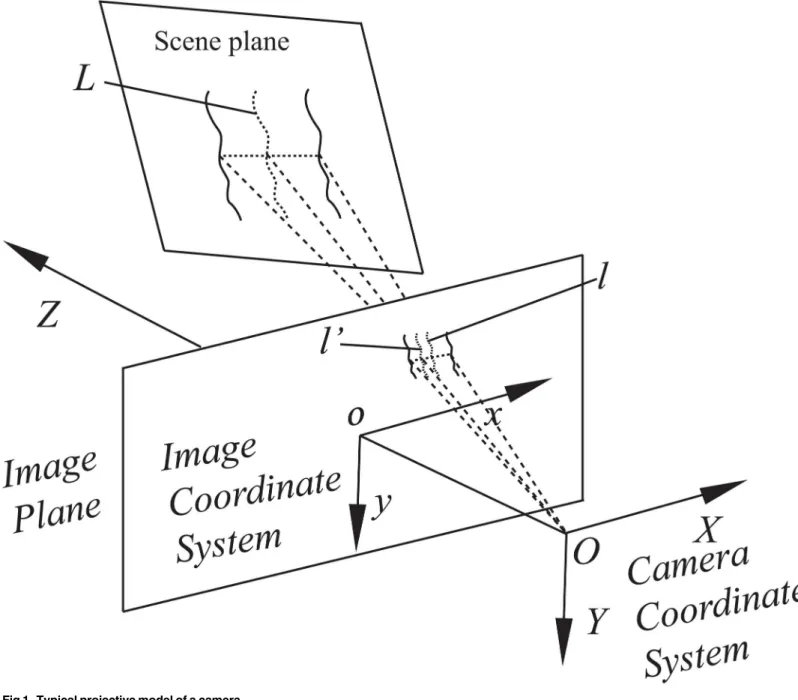
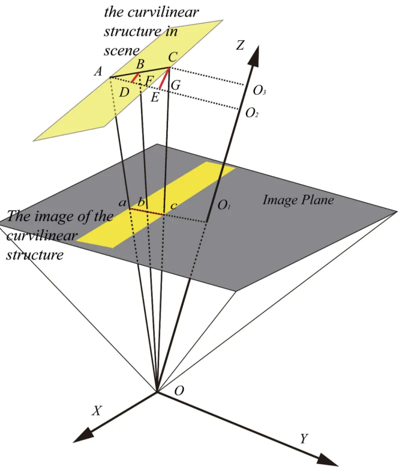
Moreover, most cameras used for capturing images are based on a projective model; there-fore, perspective distortion of the captured image is inevitable, and it results in inaccurate line extraction. The typical projective model is shown inFig 1. The centerline of a curve in the scene isL, whereas the centerline of its image isl. The linel’in the image is the projection ofL

on the image plane. Further,o-xyis the image coordinate system, whereasO-XYZis the camera coordinate system. Owing to the existence of perspective distortion, the lineslandl’are not co-incident. Similarly, a circle in the scene also suffers from the same problem. In [32], the per-spective distortion of a circular center in the image plane has been modeled. In [33], the perspective distortion of an elliptical center, which is a more general case, has been analyzed on the basis of projective transformation and analytic geometry. Thus, perspective distortion is a significant issue that needs to be rectified from the viewpoint of line extraction, especially in some industrial measurement fields that require high precision.

In this paper, we propose a new model for correcting line positions in an over-exposed image. The proposed model is based on the Gaussian model of Steger’s method, with the addi-tional capability of suitably fitting line profiles in over-exposed images. As a result of this cor-rection procedure, the center of the line profile becomes close to the ideal/actual center (as shown inFig 2). We also discuss the related properties of perspective distortion. In addition, we describe the relationship between the centerline of a scene and the centerline of its image, which can serve as a reference for correcting the bias introduced by perspective distortion. Fur-ther, we discuss the practical applications of the proposed method, including its application to vision measurement. Finally, we describe some simulations and experiments conducted to

Line Extraction Correction in Vision Measurement

professor in the School of Instrumentation Science and Opto-electronics Engineering Beihang University, China. His research interests are machine vision and artificial intelligence. Guangjun Zhang received his PhD degree from the Department of Precision Instrument Engineering of Tianjin University, China, in 1991. He was a visiting professor at North Dakota State University, USA, from 1997 to 1998. He was a Yangtze River Scholar Award Program Professor in 2000. He is currently a professor in the School of Instrumentation Science and Opto-electronics Engineering, Beihang University China and an academician of CAE. His research interests are laser precision measurement, machine vision, optical sensing, and artificial intelligence.

(3)

verify the validity of our method. Because the line position is critical in vision measurement, obtaining the line position is the primary objective of this study.

Correction of Line Position in Over-Exposed Image

A) Model description

a) Steger’s line extraction model. As lines exhibit a characteristic profile across the line at each point, the problems concerning the extraction of lines are essentially one-dimensional in nature. The related analysis can be carried out for one-dimensional line profile. When consid-ering one-dimensional line profile, a bar-sharped line model, a parabolic line model and a

Fig 1. Typical projective model of a camera.

(4)

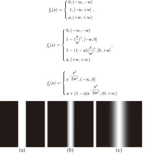
Gaussian line model are used to fit the profile and remove the bias in Steger’s method respec-tively[26,27]. The images of the three models in Steger’s method are shown inFig 3.

The functions of the three models stated in Steger’s method are listed below:fb(x) denotes the bar-shaped line profile,fp(x) denotes the parabolic line profile, andfg(x) denotes the Gauss-ian line profile.

fbðxÞ ¼

0_;_ð1_;_w_Þ

1_;_½_w;_þ_w

a;ðþw;þ1Þ

; ð1Þ

8

> <

> :

fpðxÞ ¼

0_;_ð1_;_w_Þ

1_ðx wÞ

2

;½w;0

1_ð1_a_Þðx wÞ

2

;½0_;_þ_w

a;ðþw;þ1Þ

; ð2Þ

8 > > > > > > < > > > > > > :

fgðxÞ ¼ e

x2 2_w2

;ð1;0

aþ ð1_a_Þ_e x2 2_w2

;ð0_;_þ1Þ

ð3Þ 8 > > > < > > > :

Fig 2. (a) Over-exposure image, (b) extraction result in over-exposure image.

doi:10.1371/journal.pone.0127068.g002

Fig 3. (a) Image of a bar-shaped, (b) image of a parabolic, and (c) image of a Gaussian line with equal line widths.

(5)

wherewdenotes the width of the profile anda(0a<1) denotes the asymmetry of the profile. Among these three models, the Gaussian line profile is the most precise model for line extrac-tion after correcextrac-tion, whereas the bar-shaped line profile is simplest one.

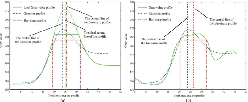
To extract the line position in an over-exposed image, the bar-shaped profile and the Gauss-ian profile are adopted to fit the profile, including the ideal and real profiles. The related fitting results are shown inFig 4.

InFig 4, there is a certain bias between the ideal center and the fitted one when either the bar-shaped line profile or the Gaussian line profile is used. Image saturation is the main reason for this phenomenon, as shown inFig 4(A). Similar problems also exist in real images, as shown inFig 4(B). Thus, the models stated in Steger’s method cannot fit the line profile in an over-exposed image properly. Therefore, a bias is introduced between the extracted center and the ideal/actual one.

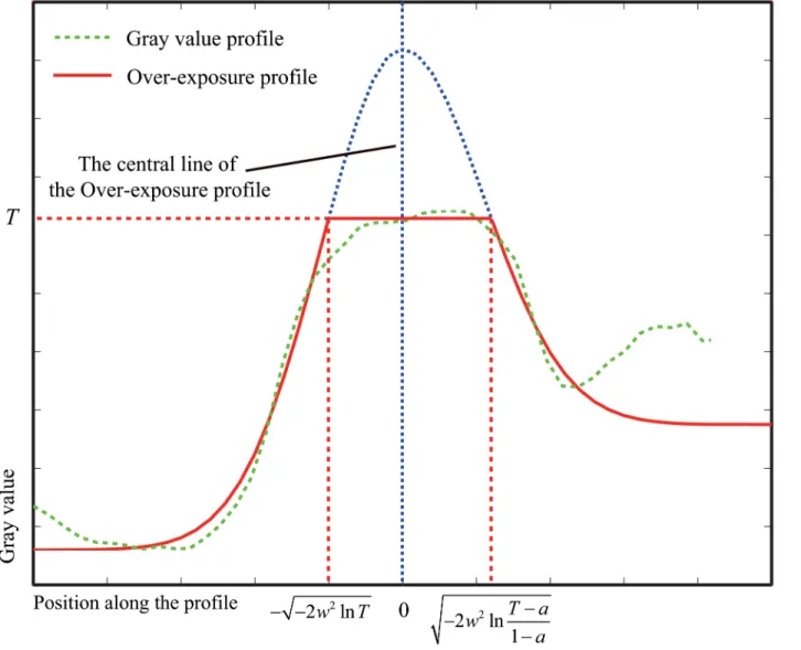
b) Over-exposure model. Owing to the saturation of over-exposed images, Steger’s line extraction models, including the bar-shaped, parabolic, and Gaussian line profiles, do not allow accurate fitting of the line profile. Therefore, we propose a new model, namely, the over-exposure model, based on Steger’s Gaussian line profile.

As shown inFig 5, let us assume thatTis the saturation value in the over-exposure model. From Eq (3),f(x) is given by

fðxÞ ¼

e x2 2_w2

;ð1; ffiffiffiffiffiffiffiffiffiffiffiffiffiffiffiffiffiffiffi 2_w2_ln

T

p

Þ

T;ð ffiffiffiffiffiffiffiffiffiffiffiffiffiffiffiffiffiffiffi 2_w2_ln

T

p

;

ffiffiffiffiffiffiffiffiffiffiffiffiffiffiffiffiffiffiffiffiffiffiffiffiffiffiffiffi 2_w2_lnTa 1_a

r

Þ

aþ ð1_a_Þ_e x2 2_w2

;ð

ffiffiffiffiffiffiffiffiffiffiffiffiffiffiffiffiffiffiffiffiffiffiffiffiffiffiffiffi 2_w2_lnTa 1_a

r

;þ1Þ

; ð4Þ

8 > > > > > > > > > < > > > > > > > > > :

whereaandware deﬁned as in Eq (3). The relation betweenTandais 1>T>a>0 in the scale

Fig 4. (a) Ideal over-exposure model and fitting result using the bar-shaped profile and the Gaussian profile, (b) line profile in the over-exposed image.

(6)

space. The description of the real profile requires a scale factor related to the description in the scale space. Thefitness of a profile in the real image using the proposed method is plotted inFig 5.

The center of the gray value profile is determined by the zero crossing of the first-order de-rivative (f’(x) = 0), i.e., the local maximum (for bright lines) or local minimum (for dark lines) of the gray value profile. For real images, this criterion must be augmented with a criterion for selecting salient lines representing the noise involved. This can be achieved with a threshold on |f”(x)|, as mentioned in Steger’s method, i.e., by requiring thatf”(x)<<0 for bright lines and

f”(x)>>0 for dark lines. Furthermore, derivatives of the real image are estimated by convolv-ing the image with the derivative of a normal Gaussian kernel [34]. The normal Gaussian ker-nel and its derivatives are given by

gðx;s_{Þ ¼} _{ffiffiffiffiffiffi}1 2_p

p

se x2

2s2_;

ð5Þ

Fig 5. Fitness of a real profile using the proposed model.

(7)

g0_ð_x;_s_{Þ ¼} x

ffiffiffiffiffiffi

2_p

p

s3e x2

2s2; ð6Þ

g00ðx;sÞ ¼x

2

s2

ffiffiffiffiffiffi

2_p

p

s5e x2

2s2_:

ð7Þ

In the scale space, the description of the proﬁle can be determined by convolving the gray value proﬁle with the corresponding derivative of the normal Gaussian kernel. The scale space de-scription is given by

rðx;s;w;a;TÞ ¼fðxÞ gðx;sÞ

¼ ffiffiffiffiffiffi

2_p

p

wgðx; ffiffiffiffiffiffiffiffiffiffiffiffiffiffiffiffi

w2

þs2

p

Þ þ ½1_apffiffiffiffiffiffi2_p_wg_ð_x; ffiffiffiffiffiffiffiffiffiffiffiffiffiffiffiffi_w2

þs2

p

Þðx2þ

xw2

w2

þs2;

ws

ffiffiffiffiffiffiffiffiffiffiffiffiffiffiffiffi

w2

þs2

p Þ

ðx1þ

xw2

w2

þs2;

ws

w2

þs2

p Þ þ ðaTÞðxx2Þ þTðxþx1Þ

; ð8Þ

r0_ð_x;_s_;_w;_a;_T_{Þ ¼}_f_ð_x_Þ_g0_ð_x;_s_Þ

2_p

p

wg0_ð_x; ffiffiffiffiffiffiffiffiffiffiffiffiffiffiffiffi

w2

þs2

p

Þ ½1_a_ð_x 2þ

xw2

w2

þs2;

ws

w2

þs2

p Þ

þgðx2þ

xw2

w2

þs2;

ws

w2

þs2

p Þ½1_apffiffiffiffiffiffi2_p_wg_ð_x; ffiffiffiffiffiffiffiffiffiffiffiffiffiffiffiffi_w2

þs2

p

Þ

w

2

w2

þs2gðx1þ

xw2

w2

þs2;

ws

w2

þs2

p Þ þ ðaTÞgðxx2Þ þTgðxþx1Þ

; ð9Þ

r00_ð_x;_s_;_w;_a;_T_{Þ ¼}_f_ð_x_Þ_g00_ð_x;_s_Þ

2_p

p

wg00_ð_x; ffiffiffiffiffiffiffiffiffiffiffiffiffiffiffiffi

w2

þs2

p

Þ ½1_a_ð_x₂_þ xw 2

w2

þs2;

ws

w2

þs2

p Þ

ð w

2

w2

þs2Þ 2

g0_ð_x 2þ

xw2

w2

þs2;

ws

w2

þs2

p Þ½1_apffiffiffiffiffiffi2_p_wg_ð_x; ffiffiffiffiffiffiffiffiffiffiffiffiffiffiffiffi_w2

þs2

p

Þ

2_apffiffiffiffiffiffi2_p_wg0_ð_x; ffiffiffiffiffiffiffiffiffiffiffiffiffiffiffiffi

w2

þs2

p

Þgðx2þ

xw2

w2

þs2;

ws

w2

þs2

p Þ w

2

w2

þs2

ð w

2

w2

þs2Þ 2

g0_ð_x 1þ

xw2

w2

þs2;

ws

w2

þs2

p Þ þ ðaTÞg0_ð_x_x

2Þ þTg0ðxþx1Þ:

; ð10Þ

The related notations are deﬁned as

x1¼

ffiffiffiffiffiffiffiffiffiffiffiffiffiffiffiffiffiffiffi 2_w2

lnT

p

;x2¼

ffiffiffiffiffiffiffiffiffiffiffiffiffiffiffiffiffiffiffiffiffiffiffiffiffiffiffiffi

2_w2

lnTa

1_a

r

; ðx;s_{Þ ¼}

Z x 1

et

2 2s2_dt:

B) Removal of bias

As the line position is the necessary information in vision measurement, we analyze the bias of the center of the profile in an over-exposed image as well as the effect of the saturation valueT. The center of the profile is determined from the zero crossing of the first-order derivative, i.e.,

r'(x,σ_,_w_,_a_,_T_{) = 0. Because direct determination is difficult, the centerline is computed using a}

(8)

method [28] in the proposed extraction method. The following proposition is obtained from [27]:if bothσ_{and w are scaled by the same constant factor s}_,_{the line and edge locations will be} sl,sel,and ser, wherelis the line position,elis the left edge point, anderis the right edge point. Thus, bias analysis can be performed forσ_{= 1, and all other values can be obtained via simple}

multiplication by the actual scaleσ_.

a) Effect ofTon bias. In this section, we analyze the effect of the parameterTon the bias, under the conditions of asymmetry and symmetry. The relationship between the convolution of the profile with the Gaussian kernel function and the parameterTis shown inFig 6.

The line position, i.e., the maximum of the profile, is invariant in the case of symmetry. In contrast, in the asymmetric condition, the maximum of the profile varies according toT. Thus, in the case of asymmetry, correction should be performed in order to obtain a precise position.

b) Correction in asymmetric condition. The profile in the over-exposure model is a part of the Gaussian line profile. Let the entire Gaussian line profile beRg(x,σ_,_w_,_a_{) and the missing}

part beRd

gðx;s;w;a;TÞ. Then, the expression forrcan be rewritten as

rðx;s;w;a;TÞ ¼fðx;s;w;a;TÞ gðx;s_{Þ ¼ ð}Rgðx;s;w;aÞ Rdgðx;s;w;a;TÞÞ gðx;sÞ:ð11Þ

WhenT<<1, the extreme point ofris not unique, i.e., the center of the proﬁle will be incor-rect. Then,Rd

gðx;s;w;a;TÞcan be substituted forf(x,σ,w,a,T), because they have the same

cen-ter point. Further, the description ofRd

gðx;s;w;a;TÞcan be determined in a similar manner as

the description off(x,σ_,_w_,_a_,_T_):

rd

gðx;s;w;a;TÞ ¼ R d

gðx;s;w;a;TÞ gðx;sÞ

¼_ðx2þ

xw2

w2

þs2;

ws

w2

þs2

p Þ _ðx1þ

xw2

w2

þs2;

ws

w2

þs2

p Þ T_ðxx2Þ þTðxþx1Þ ; _ð12Þ

Fig 6. (a) Gray value as a function ofTand positionxin the case of symmetry; (b) Gray value as a function ofTand positionxin the case of asymmetry.

(9)

rd0

gðx;s;w;a;TÞ ¼ R d

gðx;s;w;a;TÞ g0ðx;sÞ

¼gðx2þ

xw2

w2

þs2;

ws

w2

þs2

p Þ w

2

w2

þs2gðx1þ

xw2

w2

þs2;

ws

w2

þs2

p Þ

Tgðxx2Þ þTgðxþx1Þ

; ð13Þ

rd00

g ðx;s;w;a;TÞ ¼ Rdgðx;s;w;a;TÞ g00ðx;sÞ

¼ ð w

2

w2

þs2Þ 2

g0_ð_x 2þ

xw2

w2

þs2;

ws

w2

þs2

p Þ

ð w

2

w2

þs2Þ 2

g0_ð_x 1þ

xw2

w2

þs2;

ws

w2

þs2

p Þ Tg0_ð_x_x 2Þ þTg

0_ð_x_þ_x 1Þ:

; ð14Þ

The related notations are deﬁned as in Eq (10).

It is known that the edge points of the line are the zero crossings of its second-order deri-vate, while the line positions are the zero crossings of its first-order derivate. In order to elimi-nate the scale effect, the symbolλis introduced:

l_{¼ j}rd0

gðel;s;w;a;TÞj=jr d0

gðer;s;w;a;TÞj: ð15Þ

The bias function is a map fromvσandλtowσ,T, anda, wherevσis the width of the proﬁle,

i.e.,vσ= |el−er|; thus, the correction can be determined [27].

Since a function fromR2toR3can only be injective, it is difficult to analyze the bias removal function. For this reason, the parameterwis fixed, and in this case, the bias removal function is fromR2toR2, which is surjective. In our paper, we analyze only the relationships ofvσ,λ, and

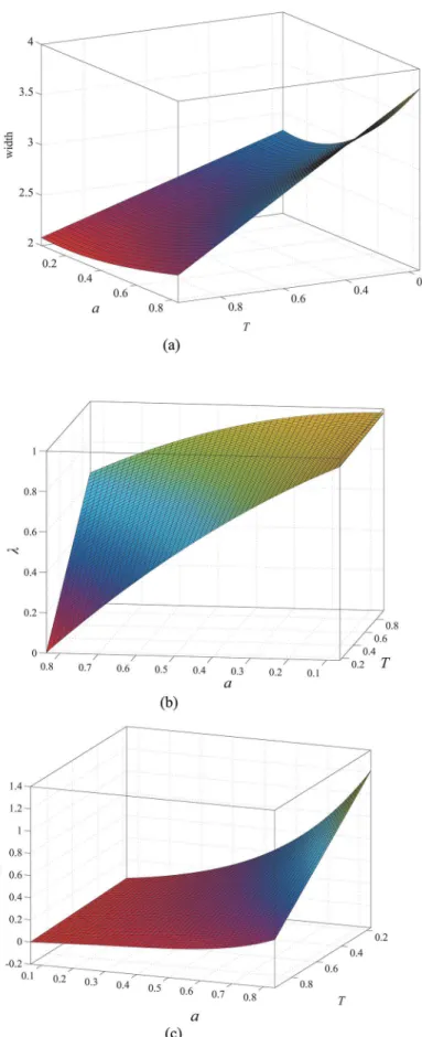
the bias with the parametersTandawhenwequals 1, 2, and 3, respectively. As in the case of the approach described in [27], the results for other values can be obtained by interpolation. The relations are shown in Figs7,8and9. Our profile involves the constraint 1>T>a>0, but the data are expanded by interpolation in these illustrations for the sake of clarity.

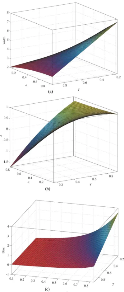
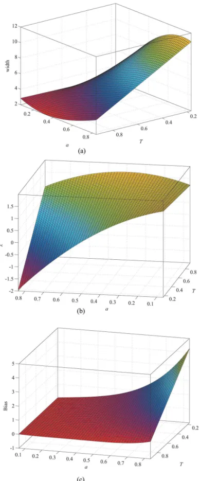
The results indicate that the line width increases asaincreases orTdecreases. Thus, the line width increases fromFig 7(A)toFig 9(A). Therefore, the line width is proportional tow. From

Fig 7(B),λincreases asadecreases orTincreases. Similarly, we can conclude thatλis propor-tional towfrom Figs7(B),8(B)and9(B). The bias, which is shown in Figs7(C),8(C)and9(C)

whenwequals 1, 2, and 3, respectively, is proportional toaandwbut inversely proportional to

T. Therefore, correction is necessary for accurate extraction of the line position, especially whenaandware too large orTis too small.

Correction of Perspective Distortion

A) Related properties

As the camera model is projective, perspective distortion exists in the captured line image, i.e., the line position of the image does not correspond with the projection of the line position of the scene on the image plane. The perspective distortion in the camera model is shown in

Fig 10.

(10)

Fig 7. Whenw= 1, (a) width as a function ofaandT; (b)λas a function ofaandT; (c) bias as a functionaandT.

(11)

Fig 8. Whenw= 2, (a) width as a function ofaandT; (b)λas a function ofaandT; (c) bias as a function ofaandT.

(12)

Fig 9. Whenw= 3, (a) width as a function ofaandT; (b)λas a function ofaandT; (c) bias as a function ofaandT.

(13)

Fig 10. Perspective distortion in the camera model.

(14)

lineAO2with lineOBand lineOC, separately. The vertical lines that pass through pointBand pointCintersect with the lineAO2at pointDand pointE, respectively. Owing to the limited field of view (FOV) of the lens, the range of angleBAD(0~90°) and angleGOO1(0~45°) can be determined; we define angleBADasθ_{, angle}_GOO₁_asβ, the width of the profile asl, and the distance from the line to the image plane asd. The following relation is obtained:

DDBF’DO2OF: ð16Þ

Then,

DB OO2

¼ DF

O2F

)lsiny=2

f þd ¼

lcosy=2_{þ j}_EF_j

ðf þdþlsinyÞtanb jEFj: ð17Þ

Therefore, the length of line segmentEFis

jEFj ¼lsinytanbðf þdþlsinyÞ lcosyðf þdÞ

lsinyþ2_ð_f_þ_d_Þ : ð18Þ

As the length of segmentEGis |EG| =lsinθ_tanβ, the following equation can be derived:

jabj jbcj¼

jAFj jFGj¼

lcosy_{þ j}EFj jEGj jEFj ¼1þ

l

f þdsiny¼1þ

jO2O3j

ðjOO1j þ jO1O2jÞ

: ð19Þ

Then, the deviation ratio is given by

t¼ l

f þdsiny¼

jO2O3j

ðjOO1j þ jO1O2jÞ

: ð20Þ

Given the width and location of the line, the derivation ratio is proportional toθ_{. Moreover,}

lines with the samez-coordinate in theCCShave the same derivation ratio.

The width of line segmentac, which is the line profile on the image plane, can be derived as follows:

f

f þd¼

jacj jAGj¼

jacj

lcosyþlsinytanb) jacj ¼

fl

f þdðcosyþsinytanbÞ: ð21Þ

The offset of the center is easily determined as

D¼ fl

2

ðfþdÞ2ðsinycosyþsin 2

ytanbÞ: ð22Þ

Asθ_andβare known, Eq (22) can be rewritten as

D¼ dfl

2

ðf þdÞ2; ð23Þ

whereδ= (sinθ_cosθ_+sin2θ_tanβ).

(15)

D0l ¼ 2_d_fl

ðfþdÞ2

D0f ¼ dl2

ðd2

f2

Þ ðf þdÞ4

D0d ¼

2_d_fl2

ðf þdÞ3

: ð24Þ

8 > > > > > > > > < > > > > > > > > :

The following properties can be deduced from Eq (24):

1. The offset is proportional toland inversely proportional tod. Further, it is proportional to the focal lengthfwhend>f, and inversely proportional tofwhend<f. In general,dis far larger thanf; therefore, the assumption that the offset is proportional tofcan be treated as a fact in practice.

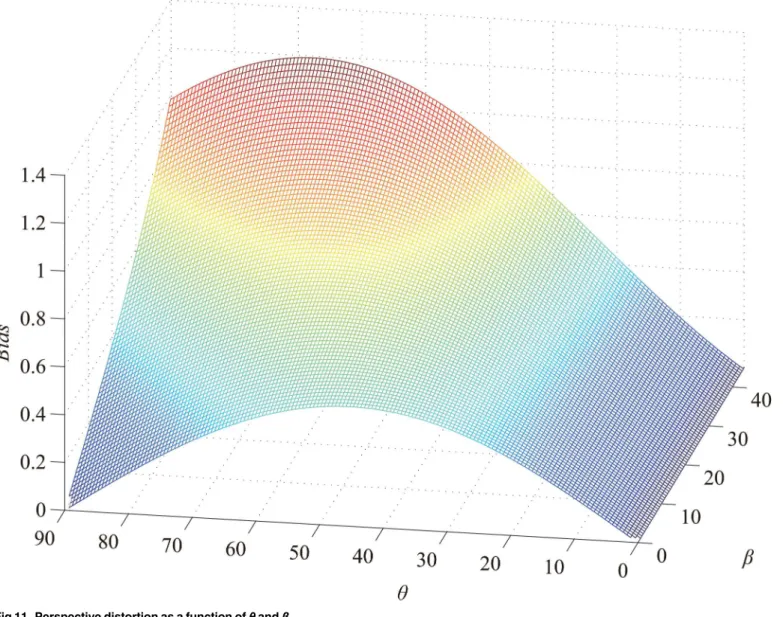
2. The offset is a function ofθ_and_β_when_f_,_l_{, and}_d_{are determined. The relationship is shown}

inFig 11.

Because we assume fl2

ðfþdÞ2to be 1 inFig 11, the offset should be multiplied by a scale factor in

practice. We can see that the offset is zero whenθ_{is zero. Although the offset is proportional to} θ_{, the available information will reduce as}_l_{decreases and}θ_{increases. Synthesizing the related}

factors,θ_{should be minimized to obtain sufficient information and decrease the offset. If}

re-quired, correction can be performed on the basis of Eq (22).

B) Perspective distortion in measurement

In this section, we consider a typical vision measurement system, namely, the line-structured light vision system (LSLVS), as an example. In the measurement process ofLSLVS, a light stripe is projected onto the target surface. The light stripe, which represents the available information, is captured for reconstruction.

The schematic ofLSLVSis shown inFig 12. The profile of the laser beam, i.e., the line seg-mentabinFig 12, can be represented as the normal Gaussian line profile. The profile of the projection on the image plane isAB. Line segmentBCis parallel to line segmentab, and it also satisfies the normal Gaussian distribution. PointDis the midpoint ofBC, while lineDFis par-allel to lineACand intersects with lineABat pointF. Because the projective angle of the laser projector (angleFinFig 12) is small (in general, around 0.02°), the line segmentABcan also be treated as the normal Gaussian line profile. Similarly, the midpoint of line segmentABcan be treated as the projection (pointE) of the center of the laser projector, i.e., pointEand point

Fare approximately coincident.

Pointa’and pointb’are the projective points of pointAand pointBon the image plane. Line segmenta’b’is not a Gaussian line profile, but it should be multiplied by a function of the Gaussian line profile. Then, the description of line segmenta’b’is given by

fðxÞ ¼ e

F

2

x2 2_w2

;ð1;sinyF

aþ ð1_a_Þ_e F2

x2 2_w2

;ðsinyF;þ1Þ

: ð25Þ

(16)

Owing to offset of the light stripe in thex-direction, Eq (25) is simplified as

fðxÞ ¼eF

2_x2

2w2; ð26Þ

whereF= cosθ_{+ sin}θ_tanβ, andθ_andβare deﬁned as inFig 10. For a vision measurement sys-tem, the normalFOVis less than 90° (e.g., a 1/3”CCDcamera with a 2.8-mm lens); similarly,β

is less than 45°. Then, Eq (26) can be rewritten as

fðxÞ ¼ ðex

2 2w2

ÞF2: ð27Þ

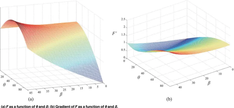
Fand its gradient as a function ofθ_andβare shown inFig 13.

InFig 13(A), the value ofFis less than 1.5. Moreover, the continuity ofFwith a small gradi-ent can be deduced fromFig 13(B). As there exists only a small variation inθ_andβintheCCS, the variation ofFis small, i.e., the offset is small. In the measurement process ofLSLVS, the width of the laser stripe is small, whereas the distance from the lens to the target (d) is much

Fig 11. Perspective distortion as a function ofθandβ.

(17)

greater than the focal length (f). Therefore, we obtain the relationship fl2

ðfþdÞ21. In other

words, the offset due to perspective distortion is small. The geometrical center of the line image

Fig 12. Schematic of line-structured light vision system.

Fig 13. (a)Fas a function ofθandβ; (b) Gradient ofFas a function ofθandβ.

(18)

can be considered as the representation of the center of the line in the scene. In some special fields that require high precision, the line position can be corrected, if required, on the basis of the method described in Section 4.

Experiment

A) Images using the over-exposure model

In this section, we explain how the over-exposure model is used to extract the line position from an over-exposed image. In the field of medical image analysis, owing to over-exposure, the image of the line is always saturated in the negative direction (Fig 14(A)). During laser

Fig 14. Application of the proposed method to (a) medical imaging (the image is taken from [27]); (b) image of a 1D target in the structured light vision system; (c) image of a planar target in the line-structured light vision system.

(19)

measurement, over-exposure is inevitable;Fig 14(B) and 14(C)show some examples. The line position is extracted using the over-exposure method, and the related results are plotted in

Fig 14.

To verify the effect of exposure level on the proposed method, images were captured under different levels of exposure.Fig 15shows the setup of the line-structured light vision system. In this system,AVT F-504Bwas employed as the camera for capturing images of the light stripe at different levels of exposure. The light stripe was projected onto the surface of an experimen-tal workpiece. By controlling the exposure time, a series of images at different exposure levels can be captured. As the camera faces the surface of the experimental workpiece, the perspective distortion is negligible in this experiment. The results are shown inFig 16.

The images captured at different levels of exposure are shown inFig 16. The exposure time of the image inFig 16(A)is 70 ms, and the gray value of the line is unsaturated. Therefore, for

Fig 16(A), extraction using the Gaussian model of Steger’s method is identical to that using the proposed method. Further, it is verified that the extraction accuracy is sufficiently high such that the obtained value can be regarded as the true value in this experiment. FromFig 16(A)to

Fig 16(F), the exposure time increases, and the exposure becomes increasingly evident. Thus,

Fig 15. Structure of the over-exposure experiment.

(20)

the centers of these images (Fig 16(B)–16(F)) can be detected by the proposed method. Unlike the method described in [27], the proposed method detects the centers according to the fitting edges of the profile, and the result obtained is compared with the true value.

In order to compare with the detected result of other methods, the extractions were also per-formed using Steger’s method and the method mentioned in [23] (inFig 16, the extractions using other methods are not plotted for the sake of clarity). The line centers using three differ-ent methods as a function of exposure time are listed inTable 1.

According toTable 1, the root mean square (RMS) error of the centers extracted by the pro-posed method is less than 0.5 pixels, while the RMS error of the centers extracted by the other two methods is less than 1.0 pixel. Although Steger’s method and the method in [23] also pro-vide good results, they are less accurate than the over-exposure model. The corrected result is more precise than the uncorrected result by around 45.5%. Thus, the proposed method is capa-ble of precisely detecting the center from an over-exposed image.

B) Correction of perspective distortion

Because it is difficult to determine the center of the line, a planar target with zebra stripes is em-ployed in our experiment. The image is captured at an angle of around 60°. In the experiment, the adjacent black and white stripes are treated as a group. In this case, the center is obvious

Fig 16. Extraction of the light stripe at different exposure levels.The green line represents the gray value of the profile, whereas the red line represents the fitting result. Extraction with exposure duration of (a) 70 ms; (b) 253 ms; (c) 590 ms; (d) 870 ms; (e) 1030 ms; (f) 2723 ms.

(21)

because of the distinct contrast between black and white. Then, the group is processed as a sin-gle color (Fig 17(A)), and the image center of the group can be determined, while the corrected center can also be determined using Eq (20). The related result is shown inFig 17.

Furthermore, a series of experiments were conducted to evaluate the effect of perspective distortion on the extraction. Because it is difficult to measure the shooting angle, we merely in-creased the angle to observe the perspective distortion. We obtained the center of the line using the extraction method and then corrected based on the related properties. The ideal center is obtained as descripted above. As the extraction method descripted in our manuscript, the cen-ter of the line at one position can be obtained from its one-dimensional line profile. In this case, the center is simplified to one-dimensional space and the results are listed inTable 2.

In general, the image center does not correspond with the projection of the scene center on the image plane. According toTable 2, the extraction is improved evidently after correction of perspective distortion. The root mean square (RMS) error of the extracted center after correc-tion is about 0.22 pixels, while the RMS error of uncorrected extraccorrec-tion is about 1.44 pixels. In our experiments, the shooting angle increases from No.1 to No.9 gradually. In order to show evidently, the perspective distortion as a function of the shooting angle is shown inFig 18.

No. Time of exposure (ms) Gaussian line proﬁle (pixel)

Method in [23] (pixel) Over-exposure model (pixel)

——— Center Error Center Error Center Error

70 43.40 ——— 43.40 ——— 43.40 ———

1 253 44.03 0.63 42.87 -0.53 43.17 -0.23

2 590 42.56 -0.85 41.98 -0.89 43.53 0.13

3 870 42.52 -0.88 41.06 -0.92 44.03 0.63

4 1030 43.10 -0.30 40.05 -1.01 44.24 0.84

5 2723 42.04 -1.36 38.78 -1.27 43.44 0.04

RMS ——— ——— 0.88 ——— 0.95 ——— 0.48

doi:10.1371/journal.pone.0127068.t001

Fig 17. Effect of perspective distortion on extraction.(a) Processed image, (b) Original image. The green circle denotes the image center, whereas the red cross denotes the corrected one.

(22)

Table 2. Extraction results and its corrected results.

No. True Value (pixel) Uncorrected (pixel) Corrected (pixel)

———— Center Error Center Error

1 52.18 52.40 0.22 52.38 0.20

2 52.18 52.64 0.46 52.36 0.18

3 52.18 52.79 0.61 52.37 0.19

4 52.18 53.15 0.97 52.40 0.22

5 52.18 53.33 1.15 52.43 0.25

6 52.18 53.54 1.36 52.35 0.17

7 52.18 54.00 1.82 52.28 0.10

8 52.18 54.38 2.20 52.45 0.27

9 52.18 54.59 2.41 52.48 0.30

RMS ———- ———- 1.44 ———- 0.22

doi:10.1371/journal.pone.0127068.t002

Fig 18. Perspective distortion as a function of the shooting angle.

(23)

shooting angle is large. After correcting based on Eq (20), the distortion is nearly eliminated. In practice, the correction should be performed according to specific requirements.

Conclusion

In this paper, we proposed a method for correcting line positions extracted from an over-ex-posed image. Based on the Gaussian line profile of Steger’s method, a new line model was de-veloped by incorporating over-exposure features. Accordingly, the proposed model was used to determine the line position from an over-exposed image. Simulations and experiments showed that the proposed model is more suitable than Steger’s method for line extraction from an over-exposed image in terms of its accuracy and its ability to detect the actual line center in the over-exposed image. We also analyzed the perspective distortion, which is inevitable during line extraction owing to the projective camera model employed in vision measurement. The perspective distortion can be rectified on the basis of the bias introduced as a function of relat-ed parameters. In addition, we discussrelat-ed the properties of the proposrelat-ed model and its applica-tion to vision measurement. In practice, a suitable model should be selected to correct line extraction, and the perspective distortion can be corrected according to specific requirements. Moreover, the proposed model can be used not only in vision measurement but also in other fields such as remote sensing and medical image analysis, where over-exposed images are frequently encountered.

Although the proposed line model is based on the Gaussian line profile, higher accuracy can be achieved by replacing the Gaussian line profile by a better extraction method. In addition, when the over-exposure is severe, the saturation value is small. In such cases, the proposed line model becomes ineffective, and it should be improved to obtain the actual line position. We plan to investigate such scenarios in future studies.

Acknowledgments

We would like to thank Dr. Y. Wang from Beihang University who helped the authors to finish the experiments. We would also like to thank one anonymous reviewer for helpful suggestions that improved this manuscript.

Author Contributions

Conceived and designed the experiments: MS ZW. Performed the experiments: MS. Analyzed the data: MS. Contributed reagents/materials/analysis tools: MS ZW GZ. Wrote the paper: MS MH.

References

1. Wessel B. Automatische Extraktion von Straβaus SAR-Bilddaten, Deutsche Geodätische Kommis-sion, Reihe C, Heft 600, München, 2006.

2. Hedman K. Statistical fusion of multi-aspect synthetic aperture radar data for automatic road extraction, Deutsche Geodätische Kommission, Reihe C, Heft 654, München, 2010.

3. Hinz S, Baumgartner A. Automatic extraction of urban road networks from multi-view aerial imagery ISPRS J. Photogramm. Remote Sens., 58 (2003), pp. 83–98.

4. Hinz S, Wiedemann C. Increasing efficiency of road extraction by self-diagnosis Photogramm. Eng. Re-mote Sens., 70 (2004), pp. 1457–1466.

5. Fleming MG, Steger C, Zhang J, Gao J, Cognetta AB, Pollak I, et al. Techniques for a structural analy-sis of dermatoscopic imagery Comput. Med. Imaging Graph., 22 (1998), pp. 375–389. PMID:9890182 6. Fleming MG, Steger C, Cognetta AB, Zhang J. Analysis of the network pattern in dermatoscopic

(24)

7. Xiong G, Zhou X, Degterev A, Ji L, Wong STC. Automated neurite labeling and analysis in fluorescence microscopy images. Cytometry Part A, 69A (2006), pp. 494–505.

8. Zhang Y, Zhou X, Witt RM, Sabatini BL, Adjeroh D, Wong STC. Dendritic spine detection using curvilin-ear structure detector and LDA classifier. NeuroImage, 36 (2007), pp. 346–360. PMID:17448688 9. Nuydens R, Dispersyn G, Kieboom GVD, de Jong M, Connors R, Ramaekers F, et al. Bcl-2 protects

against apoptosis-related microtubule alterations in neuronal cells. Apoptosis, 5 (2000), pp. 43–51 PMID:11227490

10. Wei Z, Zhou F, Zhang G. 3d coordinates measurement based on structured light sensor. Sensor Actuat. A: Phys., 120 (2005), pp. 527–535.

11. Wong AK, Niu P, He X. Fast acquisition of dense depth data by a new structured light scheme. Comput. Vision Image Understand., 98 (2005), pp. 398–422.

12. Sun J, Zhang G, Wei Z, Zhou F. Large 3d free surface measurement using a mobile coded light-based stereo vision system. Sensor Actuat. A: Phys., 132 (2006), pp. 460–471.

13. Hinz S, Stephani M, Schiemann L, Zeller K. An image engineering system for the inspection of transpar-ent construction materials. ISPRS J. Photogramm. Remote Sens., 64 (2009), pp. 297–307.

14. Lemaître C, Miteran J, Matas J. Definition of a model-based detector of curvilinear regions, in: Kro-patsch WG, Kampel M, Hanbury A (Eds.), Computer analysis of images and patterns, Lecture Notes in Computer Science, vol. 4673, Springer-Verlag, Berlin (2007), pp. 686–693.

15. Guan T, Duan LY, Yu JQ, Chen YJ, and Zhang X, Real Time Camera Pose Estimation for Wide Area Augmented Reality Applications, IEEE Computer Graphics and Application, 31(3), pp. 56–68, 2011. doi:10.1109/MCG.2010.23PMID:24808092

16. Gao Y, Wang M, Ji RR, Wu XD, Dai QH, 3D Object Retrieval with Hausdorff Distance Learning, IEEE Transactions on Industrial Electronics, 61(4), pp. 2088–2098, 2014.

17. Gao Y, Wang M, Zha ZJ, Shen JL, Li XL, Wu XD, Visual-Textual Joint Relevance Learning for Tag-Based Social Image Search, IEEE Transactions on Image Processing, 22(1), pp. 363–376, 2013. doi: 10.1109/TIP.2012.2202676PMID:22692911

18. Gao Y, Wang M, Tao DC, Ji RR, Dai QH, 3D Object Retrieval and Recognition with Hypergraph Analy-sis, IEEE Transactions on Image Processing, 21(9), pp.4290–4303, 2012. doi:10.1109/TIP.2012. 2199502PMID:22614650

19. Ji RR, Duan LY, Chen J, Yao H, Yuan J, Rui Y, Gao W, Location discriminative vocabulary coding for mobile landmark search, International Journal of Computer Vision, 96 (3), pp. 290–314, 2012. 20. Guan T, He Y, Gao J, Yang J, and Yu J, On-Device Mobile Visual Location Recognition by Integrating

Vision and Inertial Sensors, IEEE Transactions on Multimedia, 15(7), pp.1688–1699, 2013.

21. Guan T, He YF, Duan LY, and Yu JQ, Efficient BOF Generation and Compression for On-Device Mobile Visual Location Recognition, IEEE Multimedia, 21(2), pp. 32–41, 2014.

22. Guan T, Fan Y, Duan LY, On-Device Mobile Visual Location Recognition by Using Panoramic Images and Compressed Sensing Based Visual Descriptors, PLOS ONE, 9(6), 2014.

23. Jang J-H, Hong K-S. Detection of curvilinear structures and reconstruction of their regions in gray-scale images. Pattern Recognition 35 (2002) 807–824.

24. Stanford DC, Raftery AE. Finding curvilinear features in spatial point patterns: principal curve clustering with noise. IEEE Trans. Pattern Anal. Mach. Intell., 22(6), June 2000.

25. Jeon B-K, Jang J-H, Hong K-S. Road detection in spaceborne SAR images using a genetic algorithm. IEEE Trans. Geosci. Remote Sens., 40(1), Jan 2002.

26. Steger C. An unbiased detector of curvilinear structures, IEEE Trans. Pattern Anal. Mach. Intell. 20 (1998) 113–125.

27. Steger C. Unbiased extraction of lines with parabolic and Gaussian profiles. Computer Vision and Image Understanding, 117 (2013) 97–112.

28. Press WH, Numerical recipes in C: The Art of Scientific Computing, 1992.

29. Yang X, He J, Zhang G, Zhou F. A method of sub-pixel extraction from circular structured light stripes center, Opto-Electronic Engineering, 31(4), 46–49.

30. Tseng HY, Lai CH, Yu SS. An effective license-plate detection method for overexposure and complex vehicle images, ICHIT 2008: 176–181.

31. Guo D, Cheng Y, Zhuo S, Sim T. Correcting over-exposure in photographs. CVPR 2010: 515–521. 32. Heikkila J, SilvCn O. A four-step camera calibration procedure with implicit image correction. Computer

Vision and Pattern Recognition, 1997.

(25)

Science and Technology, 2003, 14:1420–1426.