Simulating snow maps for Norway: description and statistical evaluation of the seNorge snow model

(1)

TCD

6, 1337–1366, 2012

Simulating snow maps for Norway

T. M. Saloranta

Title Page

Abstract Introduction

Conclusions References

Tables Figures

◭ ◮

Back Close

Full Screen / Esc

Printer-friendly Version

Interactive Discussion

Discussion

P

a

per

|

Dis

cussion

P

a

per

|

Discussion

P

a

per

|

Discussio

n

P

a

per

|

The Cryosphere Discuss., 6, 1337–1366, 2012 www.the-cryosphere-discuss.net/6/1337/2012/ doi:10.5194/tcd-6-1337-2012

The Cryosphere Discussions

This discussion paper is/has been under review for the journal The Cryosphere (TC). Please refer to the corresponding final paper in TC if available.

Simulating snow maps for Norway:

description and statistical evaluation of

the seNorge snow model

T. M. Saloranta

Section for Glaciers, Snow and Ice, Hydrology Department, Norwegian Water Resources and Energy Directorate (NVE), Postboks 5091 Majorstua, 0301 Oslo, Norway

Received: 29 February 2012 – Accepted: 19 March 2012 – Published: 30 March 2012

Correspondence to: T. M. Saloranta (tus@nve.no)

(2)

TCD

6, 1337–1366, 2012

T. M. Saloranta

Title Page

Tables Figures

◭ ◮

Back Close

Full Screen / Esc

Discussion

P

a

per

|

Dis

cussion

P

a

per

|

Discussion

P

a

per

|

Discussio

n

P

a

per

|

Abstract

Daily maps of snow conditions have been produced in Norway with the seNorge snow model since 2004. The seNorge snow model operates with 1×1 km resolution, uses gridded observations of daily temperature and precipitation as its input forcing, and simulates among others snow water equivalent (SWE), snow depth (SD), and the snow

5

bulk density (ρ). In this paper the set of equations contained in the seNorge model code is described and a thorough spatiotemporal statistical evaluation of the model performance in 1957–2011 is made using the two major sets of extensive in-situ snow measurements that exist for Norway. The evaluation results show that the seNorge model generally overestimates bothSWE andρ, and that the distribution of model fit

10

forSWE has a clear dependency on elevation throughout the snow season. However, theR2-values for model fit are 0.60 for (log-transformed)SWEand 0.45 forρ, indicating that after removal of the detected systematic model biases (e.g. by recalibrating the model or expressing snow conditions in relative units) the model performs rather well. The seNorge model provides a relatively simple, not very data-demanding, yet still

15

process-based method to construct snow maps of high spatiotemporal resolution. It is especially well-suited alternative for operational snow mapping in regions with rugged topography and large spatiotemporal variability in snow conditions, as is the case in the mountainous Norway.

1 Introduction

20

Seasonal snow cover is an important element, and of great social and economic signif-icance in many countries, including Norway, where approximately 30 % of the annual precipitation falls as snow. Good knowledge of snow conditions is important in hy-dropower production planning, forecasting of floods and the risk of avalanches, and in water resources management. Snow conditions influence also many aspects of

so-25

ciety, such as tra_ffic flow, construction safety, winter sport activities, and play an

(3)

TCD

6, 1337–1366, 2012

T. M. Saloranta

Title Page

Tables Figures

◭ ◮

Back Close

Full Screen / Esc

Discussion

P

a

per

|

Dis

cussion

P

a

per

|

Discussion

P

a

per

|

Discussio

n

P

a

per

|

portant role in population dynamics and survival of many animal and plant species (e.g., Stenseth et al., 2004; Borgstrøm et al., 2005; Tahkokorpi et al., 2007). Conse-quently, national snow maps providing updated information on snow conditions are produced in many countries. For example, in Finland (www.fmi.fi, www.environment.fi), Sweden (www.smhi.se), Switzerland (www.slf.ch) and Canada (www.socc.ca) these

5

maps are normally constructed on the basis of (interpolated) in-situ snow observa-tions or interpreted satellite images, or a combination of both. In the United States (www.nohrsc.noaa.gov), snow maps are compiled by a rather detailed process-based energy balance model and assimilation of observations into the model simulations.

In Norway, daily maps of snow conditions have been produced at the Norwegian

10

Water Resources and Energy Directorate (NVE) with the seNorge snow model since 2004, in co-operation with the Norwegian Meteorological Institute (met.no) and the Norwegian Mapping Authority (Tveito et al., 2002; Engeset et al., 2004a, b). A model approach for snow mapping was chosen, among others, due to the lack of spatiotempo-rally well-distributed snow observation network and due to di_fficulties in using

satellite-15

based snow observations in the cloudy and mountainous Norway. The seNorge snow model operates with the same 1×1 km resolution as the model used for operational

snow mapping in the United States (see above), but is simpler and requires less forc-ing data. It simulates different snow-related variables, such as snow water equivalent (SWE), snow depth (SD), bulk snow density (ρ=SWE/SD), and the amount of liquid

20

water in snowpack (W_L), using gridded values of daily mean temperature and daily sum of precipitation as input forcing. This forcing data, produced by the met.no, is based on spatial interpolation of available temperature and precipitation observations to a grid with 1 km resolution (Tveito et al., 2005; Mohr, 2008, 2009). Consequently, a snow map consists of simulated snow conditions in approximately 324 000 1×1 km grid cells

25

(4)

TCD

6, 1337–1366, 2012

T. M. Saloranta

Title Page

Tables Figures

◭ ◮

Back Close

Full Screen / Esc

Discussion

P

a

per

|

Dis

cussion

P

a

per

|

Discussion

P

a

per

|

Discussio

n

P

a

per

|

power system planning, forecasting of runoff, floods and the risk of avalanches, in ad-dition to the public (e.g., for checking skiing conad-ditions). The historical time series of snow conditions are also applied in scientific studies.

The seNorge evaluation studies by Engeset et al. (2004b), Alfnes (unpublished NVE research note, 2008) and Stranden (2010), using snow data from point measurements,

5

snow courses, snow pillows and catchment model simulations indicated a general over-estimation ofSWE (especially in the Southern Norway) andρ, except for a few glacier sites whereSWE was generally underestimated andρstill overestimated. The overes-timation ofSWE was in these studies associated with the overestimation of the input precipitation, likely due to a too strong elevation gradient of precipitation. For the ten

10

studied stations of the hydropower companies, the annual maximumSWE was on av-erage overestimated by₊86 %, andSDsomewhat less by₊50 % due to overestimation ofρ (Stranden, 2010). However, in terms of year-to-year variation, and deviation from a long-term mean value, the evaluation of Engeset et al. (2004b) showed a rather good agreement between simulated and observedSWE.

15

Dyrrdal (2010) used observations ofSDfrom 11 meteorological stations at three dif-ferent regions and found a general underestimation ofSDon all stations for the study period 1971–2003, except for the station with highest elevation (830 m a.s.l. (above sea level)) whereSDwas overestimated. She associated the model discrepancy mainly to overestimation ofρby the snow compaction model, since the interpolated precipitation

20

was larger than the observed at most of the selected stations, while the interpolated temperature values showed good agreement with observations. Similarly, the study of Endrizzi (unpublished NVE research note, 2010) indicated a general model underesti-mation ofSDat seven meteorological stations where the model was run with observed temperature and precipitation forcing. Ragulina et al. (2011) analysed high-resolution

25

SDmeasurements (<1 m sampling interval) obtained by towing a ground-penetrating radar along approximately 80 km long transects over the Hardangervidda mountain plateau in Southern Norway in April in 2008, 2010 and 2011, approximately at the time of the maximum annualSWE. They compared the observed meanSD averaged over

(5)

TCD

6, 1337–1366, 2012

T. M. Saloranta

Title Page

Tables Figures

◭ ◮

Back Close

Full Screen / Esc

Discussion

P

a

per

|

Dis

cussion

P

a

per

|

Discussion

P

a

per

|

Discussio

n

P

a

per

|

the seNorge grid cells to the simulated values and found a general overestimation of SDby the model by roughly₊50 %.

The previous seNorge snow model evaluation studies, briefly reviewed above, indi-cate a general overestimation ofSWE andρby the model. However, the evaluations in these studies have often been rather qualitative or spatially or temporally restricted to

5

a limited number of stations or years. Since snow conditions vary strongly with region and elevation, as well as with the time and the weather characteristics of the snow season (e.g. cold and dry vs. wet and warm winters), a comprehensive set of data is needed to thoroughly spatiotemporally evaluate the seNorge snow model and the ap-proximately 20 000 daily maps of snow conditions covering the apap-proximately 324 000

10

di_fferent grid cells of Norway.

Due to the general overestimation of snow amounts in the seNorge-simulated snow maps, one has often been bound to use relative snow conditions (e.g. comparisons of current SWE to a 30-yr median SWE) instead of absolute values in practical ap-plications, such as flood forecasting and hydropower production planning. The lack of

15

accurate absolute values of snow conditions is a real limitation for many existing and potential new applications of the snow maps.

The main aim of this paper is to increase the usefulness and quality of the seNorge snow model results, and thus the snow maps for Norway, by:

– describing the set of equations contained in the seNorge model code;

20

– making a thorough statistical evaluation of the model performance in 1957–2011 using the two major sets of extensive in-situ snow measurements that exist for Norway, namely (1) the over 5 million measurements ofSDtaken at meteorologi-cal stations, and (2) the over 40 000 measurements ofSDandρ(and thusSWE) collected by various hydropower companies;

25

(6)

TCD

6, 1337–1366, 2012

T. M. Saloranta

Title Page

Tables Figures

◭ ◮

Back Close

Full Screen / Esc

Discussion

P

a

per

|

Dis

cussion

P

a

per

|

Discussion

P

a

per

|

Discussio

n

P

a

per

|

– discussing sources of uncertainty in model, input data and observations, and giv-ing suggestions for future model recalibration and development.

2 Description of the seNorge snow model

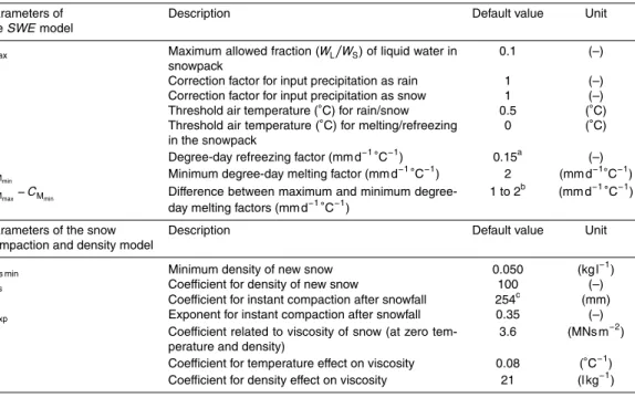
In this section the equations in the seNorge snow model code are presented. The model parameters and their default values are summarized in Table 1.

5

The seNorge snow model takes as input forcing the daily mean air temperatureT (◦ C) and the daily sum of precipitationP (mm). The model consists of two main modules: (1) theSWE model for snow pack water balance, based on the snow routine in the HBV model (Sælthun, 1996), and (2) the snow compaction and density module (Alfnes, unpublished NVE research note, 2008) used to convertSWE toSD.

10

2.1 SWE _{model for snowpack water balance}

The precipitation is categorized as liquid or solid (PL, PS) depending on whether T is

above or below the snowfall threshold temperature parameterT_S: IfT≤T_S (conditions for snowfall)

PS=fS·P

15

P_L=0 (1)

IfT > T_S(conditions for rain)

P_S=0

P_L=f_R·P (2)

20

where the parameters f_S and f_R are correction factors for the input precipitation (as snow and rain, respectively). The degree-day factorCMfor potential daily melting rate

(7)

TCD

6, 1337–1366, 2012

T. M. Saloranta

Title Page

Tables Figures

◭ ◮

Back Close

Full Screen / Esc

Discussion

P

a

per

|

Dis

cussion

P

a

per

|

Discussion

P

a

per

|

Discussio

n

P

a

per

|

between C_M

min and CMmax reaching its maximum at the summer equinox (around 21

June):

C_M=C_M_min+(C_M_max−C_M

min)·0.5·(sin(2π((Nd−81.5)/366))+1)

(3)

whereN_dis the number of the current day in the current year.

Depending on whether T is above or below the melting threshold temperature

pa-5

rameterT_M, the potential daily melting (positive values) or refreezing (negative values)

M∗ (mm d−1) in the snow pack is calculated. The actual daily melting or refreezing M

(mm d−1_{) is restricted by the availability of ice and liquid water in the snow pack,}

re-spectively:

IfT≤T_M (conditions for refreezing)

10

M∗

=C_rf(T−T_M) (4)

M=maxM∗

,−Wt−1 L

(5)

IfT > T_M(conditions for melting)

M∗

=C_M(T−T_M) (6)

15

M=minM∗ ,Wt−1

I +PS

(7)

where the superscriptstandt−1 denote values from the current (today’s) and previous

(yesterdays) time steps, and whereC_rf is a constant degree-day factor for refreezing in the snowpack. The ice content in snow (in water equivalents)WI (mm), as well as the

20

potential and actual liquid water contents in snow (W_L_pot and W_L, (mm)) are updated correspondingly:

W_Lt

pot=W

t−1

L +PL+M (8)

W_Lt=minW_Lt

pot,rmax·W

t I

(9)

W_It=Wt−1

I +PS−M (10)

(8)

TCD

6, 1337–1366, 2012

T. M. Saloranta

Title Page

Tables Figures

◭ ◮

Back Close

Full Screen / Esc

Discussion

P

a

per

|

Dis

cussion

P

a

per

|

Discussion

P

a

per

|

Discussio

n

P

a

per

|

where r_max is the maximum allowed liquid water to ice weight ratio (W_L/W_I) in the snowpack, used to restrict the actual liquid water content in snow (W_L). Note that Eq. (5) implies that only “old” W_L from previous time step can refreeze, while rain P_L in the current time step cannot refreeze.

Finally,SWE (mm) is the sum of liquid water and ice (in water equivalents) contained

5

in the snow pack, and the difference between potential and actual liquid water contents in the snow pack is lost to runo_ffQ(mm d−1):

SW Et=W_It+W_Lt (11)

Q=W_Lt

pot

−Wt

L (12)

10

2.2 Snowpack compaction and density model

The snow compaction and density model algorithms in the seNorge model are adopted from the VIC model (Cherkauer and Lettenmaier, 1999) and from the SNTHERM model (Jordan, 1991). This part of the model calculates the changes in SD (mm) in three steps. In the first step, any net decrease inSWE since the previous time step (due to

15

melting; not taking into account the new snow fallen at the current time step) is taken into account in the snow depthSD₀ by reducing SD from the previous time step with the same relative amount:

SD₀=SDt−1_·_min SW E t

−P_S

SW Et−1 , 1

!

(13)

In the second step, the lowering of the snow depth∆SD₁ due to instant compaction

20

of the old snowpack (i.e. compaction only below the new snow fall) owing to weight of new snow fallen at the current time step (if any) is calculated as in Bras (1990):

∆SD1=

P_S SW Et−P_S

·

_SD

0

b1

bexp

·SD₀ (14a)

(9)

TCD

6, 1337–1366, 2012

T. M. Saloranta

Title Page

Tables Figures

◭ ◮

Back Close

Full Screen / Esc

Discussion

P

a

per

|

Dis

cussion

P

a

per

|

Discussion

P

a

per

|

Discussio

n

P

a

per

|

whereb₁and b_expare empirical coefficients (see Table 1). After the initial compaction and added new snow, snow depthSD₁becomes thus:

SD₁=SD₀−_∆SD₁₊ PS

ρ_ns (14b)

whereρ_nsis the density of new snow fallen at the current time step (if any). The value ofρ_nsis estimated as a function of air temperature as in Bras (1990):

5

ρ_ns=ρ_{ns min}+

_max(_T

fahr, 0)

a_ns

2

(14c)

whereρ_{ns min} is the minimum density of new snow,a_nsis an empirical coefficient (see Table 1), andTfahr is the air temperature in Fahrenheit units, i.e.Tfahr=T·9/5+32.

In the third step, a gradual compaction_∆SD₂ of the whole snow pack is calculated by assuming that snow behaves as a viscous medium (e.g., Jordan, 1991):

10

∆SD₂=kc_η·g·ρw·(0.001·SW E) 0·exp(−C5·Tsnow+C6·ρ1)

·SD₁·_∆t (15a)

where the numerator describes the force (N m−2) due to the weight of the snowpack over the layer compaction is calculated for, and the denominator the viscosity of the snow (Ns m−2) as a function of snow temperatureT_snow (estimated by min (T, 0)) and densityρ₁=SW E/SD₁. Thekc,gandρware the weight scaling constant (0.5),

grav-15

itation constant (9.81 m s−2) and water density (1000 kg m−3), respectively. The η₀,C₅

andC₆are empirical coefficients (see Table 1) and∆tthe time step (s). The final snow depth and density (SDt,ρt) for the present time step are then calculated as:

SDt=SD₁−_∆SD₂ (15b)

ρt=SW E t

SDt (15c)

(10)

TCD

6, 1337–1366, 2012

T. M. Saloranta

Title Page

Tables Figures

◭ ◮

Back Close

Full Screen / Esc

Discussion

P

a

per

|

Dis

cussion

P

a

per

|

Discussion

P

a

per

|

Discussio

n

P

a

per

|

3 Model evaluation

As pointed out in Sect. 1, previous studies have indicated that the seNorge snow model tends in general to overestimate bothSWE and ρ. In order to make a statistical and more detailed evaluation of the model performance along di_fferent covariates, such as elevation and the date in the snow season (t_s), two extensive sets of in-situ snow

5

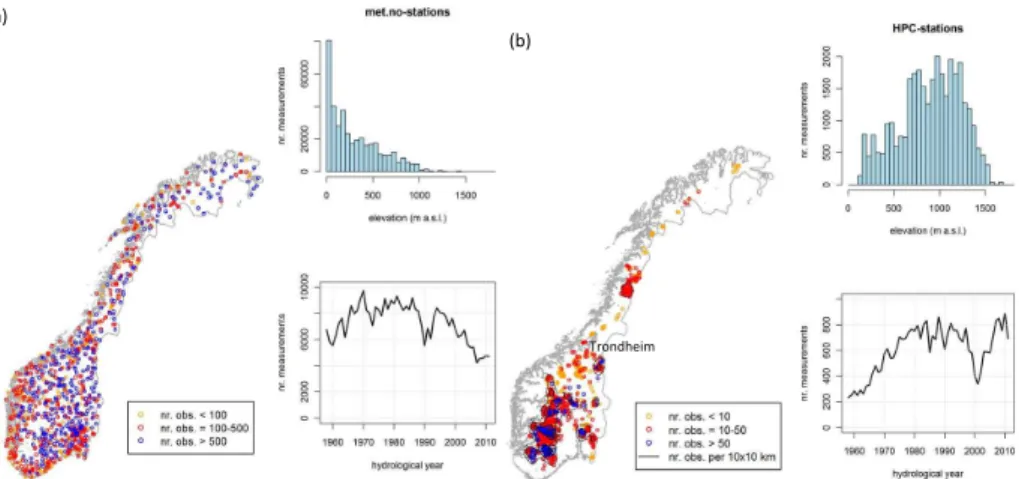
measurements for Norway are applied. The first of the snow data sets consists of daily point measurements of SD recorded at stations operated by the met.no since 1882 (hereinafter referred to as the “met.no-data”). The second data set consists of mea-surements ofSDandρ(enabling calculation ofSWE) recorded at stations operated by various hydropower companies since 1914 (hereinafter referred to as the “HPC-data”).

10

Since the seNorge snow map simulations start in 1 September 1957, data before that is not considered in the following sections. The spatiotemporal distribution and other features and differences of these two snow data sets are shown in Fig. 1 and listed in Table 2.

While the met.no-data has one hundred times more observations and a better

spa-15

tiotemporal coverage than the HPC-data,ρ has not commonly been observed at the met.no-stations, which complicates model evaluation somewhat, since a good model fit inSD can result by compensating model biases, e.g. due to overestimation in both SWE and ρ. Therefore, the HPC-data with measurements of bothSD andρis some-what better suited for seNorge model evaluation. The met.no-data also represents point

20

observations, while the HPC-data is based on mostly averages of several observations taken over a snow course, which leads to smaller uncertainty in observing the grid cell mean snow conditions. Moreover, the potential model uncertainty due to input forcing should be less at the met.no-stations than generally in model grid cells, since data from the same met.no-stations are often used in the interpolation ofT and/orP to the

25

model grid cells. Consequently, the model biases and uncertainties detected at the HPC-stations are probably more representative for the majority of the seNorge model grid cells than those detected at the met.no stations. The melting season is, however,

(11)

TCD

6, 1337–1366, 2012

T. M. Saloranta

Title Page

Tables Figures

◭ ◮

Back Close

Full Screen / Esc

Discussion

P

a

per

|

Dis

cussion

P

a

per

|

Discussion

P

a

per

|

Discussio

n

P

a

per

|

better resolved in the met.no-data. These and other sources of uncertainty are further discussed in Sect. 4. All the evaluation statistics were calculated using the “R” statistical software (www.r-project.org).

3.1 Model performance against snow data from met.no-stations

The met.no-data of dailySDmeasurements were downloaded from the met.no climate

5

data web service (eklima.met.no/wsKlima). For model evaluation purposes the data set was reduced so that measurements every 10 days were extracted from the original daily time series in 1957–2011. Since it was difficult to separate between true SD zero-values (i.e. bare ground) and missing observations, all zero or negative values in the data set were replaced by missing values, and thus only positiveSDvalues were

10

considered in the model evaluation. One clearly erroneous value was removed. The simulated SD values in grid cells corresponding to the met.no-stations were extracted from the seNorge model results, and only those grid cells, where the dif-ference between station and grid cell elevation was within±100 m, were used. After

this matching, there were 392 547 observation-simulation pairs ofSDat 1105

met.no-15

stations, which could be used in model evaluation (see Fig. 1 and Table 2). Of these, 107 267 (27 %) pairs had either the simulated or the observedSD≤10 cm. The num-ber of observations varies between 4000 and 10 000 per snow season in 1957–2011 and decreases strongly with elevation, as most of the met.no-stations are located in lowland regions (Fig. 1).

20

The overall model fit with observations was evaluated by calculating the squared correlation coe_fficient (R2-value) between simulated and observed values. TheR2was 0.61 in case of the originalSD values and 0.56 in case of the log₁₀-transformed SD values. A spline-based general additive model (GAM) fitted to the cloud of points of observed vs. simulatedSD(not shown) revealed, that the seNorge model fit switches

25

(12)

TCD

6, 1337–1366, 2012

T. M. Saloranta

Title Page

Tables Figures

◭ ◮

Back Close

Full Screen / Esc

Discussion

P

a

per

|

Dis

cussion

P

a

per

|

Discussion

P

a

per

|

Discussio

n

P

a

per

|

time of the snow season, it is important to analyse the differences between simulated and observedSD(_∆SD₌SD_sim−SD_obs) further along these three main covariates.

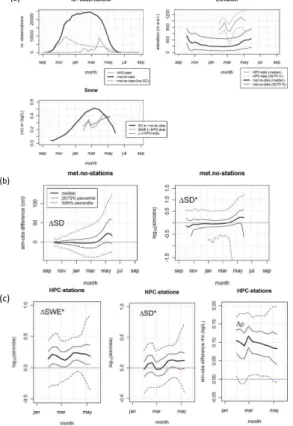
The di_fferent percentiles of the_∆SD distribution alongt_s are shown in Fig. 2. This figure shows almost no systematic bias in ∆SD, until the main melting season from the middle of March onwards, when the model starts to increasingly overestimate the

5

observed SD. However, it is worth bearing in mind, that only non-zero, positive SD values are used, and thus the number of observations varies strongly alongt_s, having a maximum around February, and being much lower both at the start and end of the snow season, as Fig. 2 shows. Moreover, the median station elevation is negatively correlated with the number of available observations, reaching a minimum elevation

10

around February.

Since the variance of _∆SD increases along t_s, an alternative model fit measure was calculated, namely the relative difference (i.e. ratio) between simulated and ob-servedSD(_∆SD∗₌SD_sim/SD_obs). As Fig. 2 shows, the variance of_∆SD∗is more con-stant alongt_s, except in the main melting season. Consequently, the relative di_fference

15

model fit measure is preferred forSDandSWE in the following model evaluations. As-suming that the station-wise log₁₀(∆SD∗) is normally distributed (visually confirmed), then Mean (log₁₀(_∆SD∗))≈Median(_∆SD∗), and an 80 % confidence factorCF_{80 %} can

be applied to describe the station-wise variability around the median value. For exam-ple, a CF_{80 %} (∆SD∗)=2 means that 80 % of the ∆SD∗ values are between 1/2 and 2

20

times the median value.

Figure 3 shows the spatial distribution (station position and elevation) of the station-wise Mean(log₁₀(∆SD∗)) for two selected dates along ts, for stations with

measure-ments from at least 15 snow seasons. Those stations where the systematic bias is not detected to be statistically significantly larger than−23 to+30 % (corresponding to

25

larger than a factor 1.3 deviation from a “perfect match”) were categorized as “good match” stations. In addition, stations at each investigated t_s (every 30 days from 30 December to 29 May) were binned by 200 m elevation intervals, and median, 10 and 90 % percentiles of the station-wise means and variability were calculated for the bins

(13)

TCD

6, 1337–1366, 2012

T. M. Saloranta

Title Page

Tables Figures

◭ ◮

Back Close

Full Screen / Esc

Discussion

P

a

per

|

Dis

cussion

P

a

per

|

Discussion

P

a

per

|

Discussio

n

P

a

per

|

containing at least 15 stations. These results show that from January through March the average station-wise Median (_∆SD∗) in all bins are within−14 to₊22 % of the exact

match, as the example for 30 March in Fig. 3 illustrates. At the end of April, however, the station-wise Median (∆SD∗) values are generally positively biased, increasingly so at higher elevations (median bias of₊25 % in the 0–200 m a.s.l. bin, and ₊108 % in

5

the 400–600 m a.s.l. bin (Fig. 3)). Similarly, from January through March the average station-wise CF_{80 %}(∆SD∗) is 1.3–2.3 (the lower the bin elevation, the higher the value), and at the end of April, somewhat higher (1.8–2.6). The percentage of “good match” stations is 72–83 % before April, but decreases to 42 % at the end of April.

Figure 3 shows also the geographical distribution of the met.no-stations whereSDis

10

significantly systematically under- or overestimated (shown for 30 March and 29 April). No very distinct clustering patterns appear, except that no significant bias is detected at a majority of the stations in the eastern, more continental half of the Southern Norway at 30 March (or before that; not shown), until the general overestimation pattern starts to prevail from April onwards.

15

3.2 Model performance against snow data from the HPC-stations

The HPC-data consists of measurements ofSD and ρ(enabling estimation of SWE) taken by various hydropower companies since the 1910s. This data is managed by NVE, where the whole data set has recently been quality controlled by removing or correcting bad or duplicate values and outliers. Only data where both SD and SWE

20

were reported in the period 1957–2011 were used in model evaluation (ρ=SWE/SD). Most of the measurements (60 %) are taken once per snow season around the time of the maximum annual SWE (March–April), but at many stations several (up to 13) measurements per snow season have been taken. A snow measurement from an HPC-station is normally based on a snow course, but may also be based on a sample taken

25

at one or more points at/around the station.

(14)

TCD

6, 1337–1366, 2012

T. M. Saloranta

Title Page

Tables Figures

◭ ◮

Back Close

Full Screen / Esc

Discussion

P

a

per

|

Dis

cussion

P

a

per

|

Discussion

P

a

per

|

Discussio

n

P

a

per

|

SDandSWEvalues in grid cells corresponding to the HPC-stations were extracted, re-sulting in 32 256 observation-simulation pairs ofSD,SWE andρat 1207 HPC-stations (see Fig. 1 and Table 2). The station elevation ranges from 139 to 1700 m a.s.l., with most of the observations located on the central mountain area in the Southern Nor-way, and most of them (70 %) taken between 600–1300 m a.s.l. (Fig. 1). The number

5

of observations varies between 200 and 900 per snow season in 1957–2011 (Fig. 1). Mostly the same methods as described in the previous section are also applied to model evaluation with the HPC-data.

TheR2-value forSWE andSD(simulated vs. observed) were 0.64 and 0.58, respec-tively (0.60 and 0.53, respecrespec-tively, in case of the log₁₀-transformed values). Forρ the

10

R2-value was 0.45. The fitted GAM-curves (not shown) revealed a general overestima-tion forSWE and SD (more so for SWE than SD, due to the parallel overestimation in ρ). The general positive bias for ρ, however, decreases towards higher values of observedρ.

As in the previous section, Fig. 2 shows the different percentiles of the distribution

15

of∆SD∗ and∆SWE∗ (=SWE_sim/SWE_obs) alongts. The same every-10-day time

res-olution is used, as with the met.no-data. However, since the HPC-data is not sampled daily, date-windows of 10 days around the dates int_s are applied to bin together ob-servations with almost equal dates. The number of stations varies strongly along ts,

as Fig. 2 shows, peaking around late March and early April, and being much lower

20

both at the start and end of the snow season. Since the motivation behind the HPC-data has mostly been to measure the annual maximum SWE, the melting season is consequently not so well resolved in this data (see Fig. 2).

Due to the lower number of stations, as well as due to variation in median elevation of the observations (Fig. 2), both∆SD∗and∆SWE∗have a more ragged pattern along

25

t_s than in the met.no data. The overall variance of _∆SD∗ and _∆SWE∗ seem to be rather invariant alongt_s, though, except in the main melting season in April, when the 5 to 95 % percentile intervals increase markedly. The median of the difference between simulated and observedρ(_∆ρ=ρ_sim−ρ_obs) reaches a maximum of₊0.12 kg l−1in early

(15)

TCD

6, 1337–1366, 2012

T. M. Saloranta

Title Page

Tables Figures

◭ ◮

Back Close

Full Screen / Esc

Discussion

P

a

per

|

Dis

cussion

P

a

per

|

Discussion

P

a

per

|

Discussio

n

P

a

per

|

March, being somewhat smaller both at the beginning and end of the snow season (Fig. 2).

Since most of the HPC-data (especially those stations with longer time series) are located in Southern Norway, this data is not as well-suited as the met.no-data for as-sessment of regional variations in the station-wise bias in model fit. Therefore, the

5

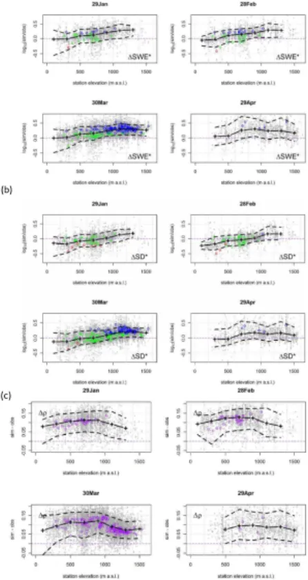
spatiotemporal analysis (i.e., calculating median, 10 and 90 % percentiles of the data in 200 m elevation-bins at different dates alongt_s) is conducted both for all data and for station-wise means. The results are shown in Fig. 4, and reveal a rather similar pat-tern for_∆SWE∗ from end of January to end of March, namely a general positive bias increasing with elevation between roughly 500–1000 m a.s.l. For example, at 30 March

10

the median bias is₊34 % and₊100 % at the bins centered at 500 and 1100 m a.s.l., re-spectively. Due to overestimation inρ(median_∆ρ∼0.1 kg l−1), the corresponding bias

for∆SD∗ is somewhat less (−5 % and+54 %, respectively). At 29 April, the significant bias in_∆SWE∗ still remains above∼500 m a.s.l. (₊50 to ₊100 %) but does not show

any clear trend with elevation anymore. The 10 and 90 % percentiles in Fig. 4 show the

15

variability in model fit. At 30 March, for example, 80 % of all the simulatedSWE values between 400–600 m a.s.l. are within−22 % and +139 % of the observed SWE in the

HPC-data, which corresponds to a CF_{80 %}of 1.7–1.8 around the median bias of₊34 %. The percentage of “good match” HPC-stations (see definition in previous section) for SWE was 57 % and 28 % in 28 February and 30 March, respectively.

20

The large-scale regional di_fferences in_∆SWE∗ were roughly investigated by remov-ing all data in the Southern Norway (south of Trondheim; see Fig. 1). Although the data coverage in the Northern Norway is rather limited (5 % of all data), the results (not shown) did not indicate any less bias inSWE than seen in the whole dataset. A plot similar to Fig. 4 showed a median bias of+76 and+57 % at 30 March in elevation bins

25

(16)

TCD

6, 1337–1366, 2012

T. M. Saloranta

Title Page

Tables Figures

◭ ◮

Back Close

Full Screen / Esc

Discussion

P

a

per

|

Dis

cussion

P

a

per

|

Discussion

P

a

per

|

Discussio

n

P

a

per

|

4 Discussion

There are several possible sources of uncertainty to explain the di_fferences seen be-tween the simulated and observed snow conditions in the two previous sections. Firstly, there is the uncertainty connected to the seNorge model structure (process represen-tation, subgrid variability), model parameters, and model input forcing (i.e. observations

5

ofP andT and their interpolation to grid cells). Secondly, there is the uncertainty con-nected to the spatial natural variability in snow conditions (horizontally and with eleva-tion), and to the snow observations (especially density can sometimes be demanding to measure).

As summarized in Table 2, the two data sets differ in many ways from each other.

10

The HPC-data seems to give a more representative picture of the seNorge model fit in Norway in general than the met.no-data, since the interpolation uncertainty in the forcing data at the met.no-stations is likely smaller than in most of the other model grid cells (see Sect. 3). Moreover, since the met.no-data consist of point observations, they have larger uncertainty in representing the grid cell mean snow conditions than the

15

HPC-data, which is based on mostly averages over a snow course. On the other hand, due to less uncertainty in the forcing data, the met.no-data could provide a better basis for isolating the uncertainty connected to the model structure and parameters, had it not been for the fact that the lack of measurements ofρmakes the model evaluation more di_fficult, since a good fit forSDcan arise from compensating biases in simulating

20

SWE andρ.

The results presented in the previous sections confirm the general and sometimes rather substantial overestimation ofSWE and ρ, which has been pointed out by pre-vious evaluation studies (Sect. 1). However, this study has contributed to refining and quantifying the knowledge on the seNorge model performance by revealing the

de-25

pendencies of the model fit by region, by the date of the snow season, and especially by elevation. Although 60 % of the area of Norway is located below 600 m a.s.l., the higher elevation regions are of special interest for e.g. hydropower production. Since

(17)

TCD

6, 1337–1366, 2012

T. M. Saloranta

Title Page

Tables Figures

◭ ◮

Back Close

Full Screen / Esc

Discussion

P

a

per

|

Dis

cussion

P

a

per

|

Discussion

P

a

per

|

Discussio

n

P

a

per

|

the positive bias forSWE increases with elevation, it could be, as indicated by previ-ous studies, that the elevation-dependency in the interpolation of the forcing data is too strong for precipitation and/or temperature, leading to increasingly excessive snow production along increased grid cell elevation. Other elevation-dependent processes (or lack of them) responsible for the increasing bias along elevation could be e.g. the

5

missing simulation of wind effects in the seNorge model, such as sublimation in blow-ing snow. Wind certainly also redistributes snow within a grid cell, but the transport of snow between the grid cells is probably negligible. Armstrong and Brun (2008) re-viewed some blowing snow model studies for Arctic regions, which showed that loss by sublimation could be 9 to 47 % of annual snowfall, depending on the topography and

10

vegetation type. Thus, although sublimation could account for a fraction of the overes-timation inSWE it seemingly cannot alone explain losses of the order of what is shown in Fig. 4.

The evaluation results with the HPC-data indicate thatρis overestimated also in the lower elevations, thus indicating that the rather good model fit seen for theSD in the

15

met.no-data might be coupled with an overestimation ofSWE. However, it is difficult to confirm this due to low number of lowland HPC-data, and since measurements ofρare generally lacking below 200 m a.s.l., where the seasonal evolution of theρand SWE may be characterized by many accumulation and melting periods, and thus be different from the higher, more alpine and stable snow climate. The overestimation ofρdoes not

20

seem to be caused by the overestimation ofSWE though (i.e. due to more overburden weight in the snow pack and thus more compation), as the lacking coherence between these variables in Fig. 4 indicates.

In the melting season (as illustrated by the di_fference from 30 March to 29 April in Figs. 3 and 4) the spread in ∆SWE∗ increases in the HPC-data, while the bias

25

(18)

TCD

6, 1337–1366, 2012

T. M. Saloranta

Title Page

Tables Figures

◭ ◮

Back Close

Full Screen / Esc

Discussion

P

a

per

|

Dis

cussion

P

a

per

|

Discussion

P

a

per

|

Discussio

n

P

a

per

|

rather decreasing along the melting season (Fig. 4). There is indication for increased bias during the melt season also in the HPC-data at the lower elevations below ca. 1000 m a.s.l. However, it is worth bearing in mind that the melt season is not as well represented in the HPC-data as in the met.no-data, and that the number of stations decreases strongly from the end of March to the end of April in the HPC-data.

5

Despite of the rather substantial biases, the seNorge model describes rather well the variability in snow conditions, as theR2 values indicate (53–60 % of the observed variance in log-transformed SWE and SD are explained by the model). One way of utilizing this strength of the model is to use the snow simulations in a relative sense, e.g. by calculating the ratio between currentSWE in a grid cell and a corresponding

10

long-term medianSWE. In these relative units most of the systematic bias is removed. For example at 30 March , in the 1000–1200 m a.s.l. bin, the 80 % confidence range for

∆SWE∗is+26 to+203 % (Fig. 4), while when using station-wise relative units (stations with at least 15 yr of observations included) the bias is removed and 80 % confidence range is now−28 to₊38 % (similarly,−25 to₊45 % in the lower 400–600 m a.s.l. bin).

15

For comparison we tested also whether an empirical statistical snow density model, e.g. that of Sturm et al. (2010), would perform better than the process-based density algorithm in the seNorge model. The model by Sturm et al. (2010), which estimatesρ

as a function of snow climate type (alpine assumed in our case),SDand the day of the year, showed less bias than the seNorge density model (+0.04 vs.+0.1 kg l−1), but the

20

variability inρ was still better simulated in the seNorge model (R2=0.45) than in the model by Sturm et al. (2010) (R2=0.32).

As already pointed out above, the observational uncertainty is largest for the point observations, but neither a mean over a snow course can give a “true” mean of the snow conditions within e.g. a 1×1 km grid cell. Thus, even with a hypothetical perfect

25

model, no perfect match with observations can be expected. Considerable spatial sub-grid variability inSWE andSDis caused among others by local precipitation patterns, and by wind redistribution of snow which again is dependent on the type of vegetation and topography (e.g., Armstrong and Brun, 2008). As an example of the observational

(19)

TCD

6, 1337–1366, 2012

T. M. Saloranta

Title Page

Tables Figures

◭ ◮

Back Close

Full Screen / Esc

Discussion

P

a

per

|

Dis

cussion

P

a

per

|

Discussion

P

a

per

|

Discussio

n

P

a

per

|

uncertainty, the high-resolutionSDmeasurements across the Hardangervidda moun-tain plateau (Ragulina et al., 2011; see Sect. 1) showed that a single point measure-ment ofSDhas typically an 80 % confidence range of−60 to+70 % in estimating the mean SD over 1 km subsections of the approximately 80 km long transects. By replac-ing the sreplac-ingle point measurement by a mean over a snow course, (by takreplac-ing a meanSD

5

of 30 samples) the typical 80 % confidence range is reduced to±10 %. This example il-lustrates the generally better accuracy in the HPC-data, which is mostly based on snow courses, than in the point measurements ofSDtaken at the met.no-stations. The con-fidence ranges in the above example apply for a treeless and hilly terrain over 1000 m a.s.l., and represent likely an upper range of variability in Norway, though. Subgrid

vari-10

ability in SD is likely somewhat smaller at the lower-lying met.no-stations, where the wind redistribution effect may be less pronounced and where the location of the snow stakes is fixed and can (in principle) be selected to be as representative as possible for the surrounding terrain.

The high-resolution SD data from the transects across Hardangervidda (Ragulina

15

et al., 2011) were also compared to seNorge model-simulated values, and the resulting

∆SD∗ values were very similar to those seen for the HPC-data. To illustrate the e_ffect of bias correction: if the seNorge simulation results were corrected for the₊54 % bias indicated by the HPC-data (at 30 March in the 1000–1200 m a.s.l. elevation bin), then the observed mean SD for the Hardangervidda transects from 2008, 2010 and 2011

20

were over-/underestimated by the seNorge model only by₊5 %,−13 % and−10 %,

re-spectively. This also indicates that the averaging over several model grid cells reduces the variability in the model fit, as compared to the grid cell-wise evaluation results pre-sented in this paper.

It is clear that the seNorge snow model needs at least a recalibration, or maybe also

25

(20)

TCD

6, 1337–1366, 2012

T. M. Saloranta

Title Page

Tables Figures

◭ ◮

Back Close

Full Screen / Esc

Discussion

P

a

per

|

Dis

cussion

P

a

per

|

Discussion

P

a

per

|

Discussio

n

P

a

per

|

equifinality problem, see e.g. Beven, 2006), the calibration method should be able to search for all plausible combinations of the model parameters that can give statisti-cally optimal model fit with the observations, taking into account also the uncertainty connected to the observations. One method that has shown to be able to fullfill these calibration requirements is the Markov chain Monte Carlo simulation (e.g., Gamerman,

5

1999; Saloranta et al., 2009).

The data presented in this paper can serve as a benchmark data set, against which new seNorge model calibrations and developments, or even new alternative model codes, can be tested and evaluated. Moreover, the results can be used in intercompar-ison of the accuracies in different snow map production methods. The seNorge snow

10

mapping method is seemingly only applied in Norway at present, but it could relatively easily be applied and tested in other countries too, especially where rugged topography and lack of observations hampers the regular use of interpolation and satellite-based snow mapping methods. Moreover, the estimated daily precipitation in the model grid cells, which is usually a crucial forcing factor in snow models, seems to be more

ac-15

curately estimated by the interpolation routines (Tveito et al., 2005; Mohr, 2008, 2009) than e.g. by numerical weather prediction models (T. Skaugen, personal communica-tion, 2012). The results in this paper can also provide an indirect evaluation of the griddedT andP data used for model forcing, especially at the HPC-stations which are often located far outside the met.no station network.

20

While waiting for the revised/recalibrated version of the seNorge model (a natural next step from this study), the bias-corrected or relative seNorge simulation results are recommended to be used, in order to increase the quality of the information on snow conditions from the snow maps of Norway.

5 Conclusions

25

Owing to the large spatiotemporal variability of snow conditions in the mountain-ous Norway, the snow maps simulated by the seNorge model provide probably the

(21)

TCD

6, 1337–1366, 2012

T. M. Saloranta

Title Page

Tables Figures

◭ ◮

Back Close

Full Screen / Esc

Discussion

P

a

per

|

Dis

cussion

P

a

per

|

Discussion

P

a

per

|

Discussio

n

P

a

per

|

best overview of the current and past snow conditions for Norway in general. This snow map production method is relatively simple, not very data-demanding, yet still process-based and able to provide snow maps of high spatiotemporal resolution (daily, 1 km×1 km grid cell).

The statistical evaluation of the seNorge snow model against the two large and

5

mostly non-overlapping datasets from the HPC- and met.no-stations has revealed and quantified the model performance, i.e. the variability and biases between the model simulations and the observations in the corresponding model grid cells. The HPC-data shows that the seNorge model generally overestimatesSWE, and that the distribution of model fit forSWE shows a clear dependency on elevation throughout the season.

10

Especially between roughly 500–1000 m a.s.l. the model bias clearly increases (or be-comes less negative) with elevation. Thus, e.g. around 30 March, the model overesti-matesSWE on average by+34 % in the 400–600 m a.s.l. bin, while by 100 % in the higher elevation 1000–1200 m a.s.l. bin. There is no clear seasonal variation in the model fit with the HPC-data. Moreover, the seNorge model overestimatesρ on

aver-15

age by approximately 0.1 kg l−1, and there is only a moderate variation in the model fit along the snow season and elevation forρ.

The R2-values of 0.60 and 0.45 for log-transformed SWE and ρ, respectively, indi-cate that the model performs rather well in simulating the observed variability inSWE andρ, despite of the overestimation of absolute values. Consequently, the uncertainty

20

in model results can be significantly reduced by using relative units where currentSWE is expressed e.g. as a fraction of a long-term median value. In this way the bias in the simulation results is mostly removed and in 80 % the cases the model results match the observed relativeSWE within a factor of roughly 1.5 in both directions. By taking areal averages over several grid cells, these confidence intervals seem to be further

25

reduced.

(22)

TCD

6, 1337–1366, 2012

T. M. Saloranta

Title Page

Tables Figures

◭ ◮

Back Close

Full Screen / Esc

Discussion

P

a

per

|

Dis

cussion

P

a

per

|

Discussion

P

a

per

|

Discussio

n

P

a

per

|

of the density algorithms (Eqs. 13–15), in order diminish the positive model bias inρ, (2) calibration of the degree-day factorsC_M, in order diminish the positive model bias inSD (andSWE) in the melting season, as seen especially in evaluation against the met.no-data, and (3) closer investigation of which elevation dependencies (or lack of them) in the model or forcing data could best explain and diminish the increasing positive model

5

bias inSWE with elevation.

Acknowledgements. Very special thanks for the various hydropower companies and for the

Norwegian Meteorological Institute (met.no) for provision of data, as well as for the seNorge model and code developers, including Eli Alfnes, Jess Andersen, Rune Engeset, Ingjerd Had-deland, Zelalem Mengistu and Hans Christian Udnæs. Thanks also to Ragnar Ekker for helping

10

downloading the data from met.no.

References

Alfnes, E.: Snow depth algorithms – compaction of snow, unpublished research note, Norwe-gian Water Resources and Energy Directorate (NVE), 2008.

Armstrong. R. L. and Brun, E.: Snow and Climate, Cambridge University Press, Cambridge,

15

86–91, 2008.

Beven, K.: A manifesto for the equifinality thesis, J. Hydrol., 320, 18–36, 2006.

Borgstrøm, R. and Museth, J.: Accumulated snow and summer temperature – critical factors for recruitment to high mountain populations of brown trout (Salmo trutta L.), Ecol. Freshw. Fish, 14, 375–384, 2005.

20

Bras, R. L.: Hydrology: an Introduction to Hydrologic Science, Addison-Wesley, Reading, UK, 643 pp., 1990.

Cherkauer, K. A. and Lettenmaier, D. P.: Hydrologic effects of frozen soils in the upper Missis-sippi River Basin, J. Geophys. Res., 104, 19599–19610, 1999.

Dyrrdal, A. V.: An evaluation of Norwegian snow maps: simulation results versus observations,

25

Hydrol. Res., 41, 27–37, 2010.

Endrizzi, S.: Verification of the seNorge snow model in point mode, unpublished research note, Norwegian Water Resources and Energy Directorate (NVE), 2010.

(23)

TCD

6, 1337–1366, 2012

T. M. Saloranta

Title Page

Tables Figures

◭ ◮

Back Close

Full Screen / Esc

Discussion

P

a

per

|

Dis

cussion

P

a

per

|

Discussion

P

a

per

|

Discussio

n

P

a

per

|

Engeset, R., Tveito, O. E., Alfnes, E., Mengistu, Z., Udnæs, H.-C., Isaksen, K., and Førland, E. J.: Snow map system for Norway, XXIII Nordic Hydrological Conference, 8–12 August 2004, Tallinn, Estonia, NHP report 48, 112–121, available online at: http://senorge. no/senorgeAux/NHC2004Tallinn SnowMapSystem Paper.pdf, last access: 29 March, 2012, 2004a.

5

Engeset, R., Tveito, O. E., Udnæs, H.-C., Alfnes, E., Mengistu, Z., Isaksen, K., and Førland, E. J.: Snow map validation for Norway, XXIII Nordic Hydrological Conference, 8–12 August 2004, Tallinn, Estonia, NHP report 48, 122–131, available online at: http://senorge.no/ senorgeAux/NHC2004Tallinn SnowMapValidation Paper.pdf, last access: 29 March, 2012, 2004b

10

Gamerman, D.: Markov Chain Monte Carlo: Stochastic Simulation for Bayesian Inference, Chapman and Hall, London, 1999.

Jordan, R.: A one-dimensional temperature model for a snow cover: technical documentation for SNTHER M.89, Special Report 91–16, US Army Cold Regions Research and Engineering Laboratory, Hanover, NH, 49 pp., 1991.

15

Mohr, M.: New routines for gridding of temperature and precipitation observations for “seNorge.no”, met.no note 08/2008, The Norwegian Meterological Institute, 40 pp., available online at: http://met.no/Forskning/Publikasjoner/Publikasjoner 2008/filestore/ NewRoutinesforGriddingofTemperature.pdf, last access: 29 March, 2012, 2008.

Mohr, M.: Comparison of versions 1.1 and 1.0 of gridded temperature and precipitation data

20

for Norway, met.no note 19/2009, The Norwegian Meterological Institute, Oslo, Norway, 44 pp., 2009, available online at: http://met.no/Forskning/Publikasjoner/Publikasjoner 2009/ filestore/note19-09.pdf, last access: 29 March 2012, 2009.

Ragulina, G., Melvold, K., and Saloranta, T.: GPR-measurements of snow distribution on Hardangervidda mountain plateau in 2008–2011, Oslo, Norway, NVE-report 8–2011, 32 pp.,

25

2011.

Saloranta, T. M., Forsius, M., J ¨arvinen, M., and Arvola, L.: Impacts of projected climate change on the thermodynamics of a shallow and a deep lake in Finland: model simulations and Bayesian uncertainty analysis, Hydrol. Res., 40, 234–248, 2009.

Stenseth, N. C., Shabbar, A., Chan, K., Boutin, S., Rueness, E. K., Ehrich, D., Hurrell, J. W.,

30

(24)

TCD

6, 1337–1366, 2012

T. M. Saloranta

Title Page

Tables Figures

◭ ◮

Back Close

Full Screen / Esc

Discussion

P

a

per

|

Dis

cussion

P

a

per

|

Discussion

P

a

per

|

Discussio

n

P

a

per

|

Stranden, H. B.: Evaluering av seNorge: data versjon 1.1. Dokument nr 4/2010, Norges vassdrags- og energidirektorat (NVE), 36 pp., (in Norwegian), available online: http://www.nve.no/Global/Publikasjoner/Publikasjoner2010/Rapport2010/rapport2010 04. pdf, 2010.

Sturm, M., Taras, B., Liston, G. E., Derksen, C., Jonas, T., and Lea, J.: Estimating snow water

5

equivalent using snow depth data and climate classes, J. Hydrometeorol., 11, 1380–1394, 2010.

Sælthun, N. R.: The “Nordic” HBV model, Publication nr. 7, The Norwegian Energy and Water Resources Administration (NVE), Oslo, Norway, 26 pp., 1996.

Tahkokorpi, M., Taulavuori, K., Laine, K., and Taulavuori, E.: After-effects of drought-related

10

winter stress in previous and current year stems of Vaccinium myrtillus L., Environ. Exp. Bot., 61, 85–93, 2007.

Tveito, O. E., Udnæs, H.-C., Mengistu, Z., Engeset, R., and Førland, E. J.: New snow maps for Norway, Proceedings XXII Nordic Hydrological Conference 2002, 4–7 August 2002, Røros, Norway, 527–532, available online at: http://senorge.no/senorgeAux/NHC2002Roros

15

NewSnowMap Paper.pdf, last access: 29 March 2012, 2002.

Tveito, O. E., Bjørdal, I., Skjelv ˚ag, A. O., and Aune, B.: A GIS-based agro-ecological decision system based on gridded climatology, Meteorol. Appl., 12, 57–68, 2005.

(25)

TCD

6, 1337–1366, 2012

T. M. Saloranta

Title Page

Tables Figures

◭ ◮

Back Close

Full Screen / Esc

Discussion

P

a

per

|

Dis

cussion

P

a

per

|

Discussion

P

a

per

|

Discussio

n

P

a

per

|

Table 1.The 15 seNorge snow model parameters with their default values and units.

Parameters of Description Default value Unit

theSWEmodel

r_max Maximum allowed fraction (W_L/W_S) of liquid water in snowpack

0.1 (–)

f_r Correction factor for input precipitation as rain 1 (–) f_s Correction factor for input precipitation as snow 1 (–) T_S Threshold air temperature (◦

C) for rain/snow 0.5 (◦

C) T_M Threshold air temperature (◦

C) for melting/refreezing in the snowpack

0 (◦

C)

C_rf Degree-day refreezing factor (mm d−1◦_C−1₎ _0.15a _(–) C_M_min Minimum degree-day melting factor (mm d−1◦_C−1₎ ₂ _{(mm d}−1◦_C−1₎ C_M_max−C_M_min Difference between maximum and minimum

degree-day melting factors (mm d−1◦

C−1₎

1 to 2b (mm d−1◦_C−1₎

Parameters of the snow Description Default value Unit compaction and density model

ρns min Minimum density of new snow 0.050 (kg l

−1₎ a_ns Coefficient for density of new snow 100 (–) b₁ Coefficient for instant compaction after snowfall 254c (mm) b_exp Exponent for instant compaction after snowfall 0.35 (–) η₀ Coefficient related to viscosity of snow (at zero

tem-perature and density)

3.6 (MNs m−2₎

C5 Coefficient for temperature effect on viscosity 0.08 (

◦

C−1₎ C6 Coefficient for density effect on viscosity 21 (l kg

−1₎

a

Default value from the HBV model (Sælthun, 1996).

b_{Grid cell specific default values are applied for}_C

Mmaxdepending on the latitude and land cover (forest) of the grid cell.

c

(26)

TCD

6, 1337–1366, 2012

T. M. Saloranta

Title Page

Tables Figures

◭ ◮

Back Close

Full Screen / Esc

Discussion

P

a

per

|

Dis

cussion

P

a

per

|

Discussion

P

a

per

|

Discussio

n

P

a

per

|

Table 2.Features of the two snow data sets used in the seNorge model evaluation (data since 1 September 1957 is considered).SD,SWEandρdenote snow depth, snow water equivalent and bulk density, respectively, and “m a.s.l.” elevation (meters above sea level).

Features met.no-data HPC-data

Sampled variables SD(only positive values, and stations with at least 10 measurements consid-ered here)

SD and ρ (enabling calculation of

SWE; only positive values considered here)

Measurement frequency every 10 days, extracted from time se-ries of daily measurements

1–13 measurements per snow season, most of them around the time of the an-nual maximumSWE

Number of measurements 392 547 samples at 1105 stations 32 256 samples at 1207 stations Type of measurements point measurement mostly average of multiple

measure-ments, e.g. over a snow course Elevation range1 mostly lowland locations (75 % of data

is from stations below 480 m a.s.l.)

mostly highland locations (75 % of data is from stations above 680 m a.s.l.) Interpolation uncertainty in

forcing data

often same stations as used in inter-polation of seNorge forcing grid-data (i.e. less interpolation uncertainty ofT and/orP at station locations)

stations located outside met.no station network (i.e. more interpolation uncer-tainty in gridded values ofT andP at station locations)

Observed range, min-max (median)

SD: 1–490 cm (32 cm) SD: 0.2–570 cm (100 cm)

SWE: 0.1–285 cm (31 cm) ρ: 0.065–0.736 kg l−1

(0.321 kg l−1

) Simulated range (seNorge),

min-max (median)

SD: 0–393 cm (33 cm) SD: 0–730 cm (129 cm)

SWE: 0–402 cm (54 cm) ρ: 0.143–0.667 kg l−1

(0.421 kg l−1

)

1_{As a comparison: 60 % of the area of Norway is located below 600 m a.s.l., and 20 % above 900 m a.s.l.}

(27)

TCD

6, 1337–1366, 2012

T. M. Saloranta

Title Page

Tables Figures

◭ ◮

Back Close

Full Screen / Esc

Discussion

P

a

per

|

Dis

cussion

P

a

per

|

Discussion

P

a

per

|

Discussio

n

P

a

per

|

(a)

(b)

Trondheim