Attribution of atmospheric sulfur dioxide over the English Channel
to dimethyl sulfide and changing ship emissions
Mingxi Yang, Thomas G. Bell, Frances E. Hopkins, and Timothy J. Smyth Plymouth Marine Laboratory, Prospect Place, Plymouth, PL1 3DH, UK
Correspondence to:Mingxi Yang ([email protected]) and Thomas G. Bell ([email protected]) Received: 19 January 2016 – Published in Atmos. Chem. Phys. Discuss.: 25 January 2016 Revised: 8 April 2016 – Accepted: 11 April 2016 – Published: 18 April 2016
Abstract. Atmospheric sulfur dioxide (SO2)was measured continuously from the Penlee Point Atmospheric Observa-tory (PPAO) near Plymouth, United Kingdom, between May 2014 and November 2015. This coastal site is exposed to ma-rine air across a wide wind sector. The predominant south-westerly winds carry relatively clean background Atlantic air. In contrast, air from the southeast is heavily influenced by exhaust plumes from ships in the English Channel as well as near Plymouth Sound. A new International Maritime Or-ganization (IMO) regulation came into force in January 2015 to reduce the maximum allowed sulfur content in ships’ fuel 10-fold in sulfur emission control areas such as the English Channel. Our observations suggest a 3-fold reduction in ship-emitted SO2from 2014 to 2015. Apparent fuel sulfur content calculated from coincidental SO2and carbon dioxide (CO2) peaks from local ship plumes show a high level of compli-ance to the IMO regulation (> 95 %) in both years (∼70 % of ships in 2014 were already emitting at levels below the 2015 cap). Dimethyl sulfide (DMS) is an important source of atmospheric SO2even in this semi-polluted region. The rel-ative contribution of DMS oxidation to the SO2burden over the English Channel increased from about one-third in 2014 to about one-half in 2015 due to the reduction in ship sulfur emissions. Our diel analysis suggests that SO2 is removed from the marine atmospheric boundary layer in about half a day, with dry deposition to the ocean accounting for a quarter of the total loss.
1 Introduction
The trace gas sulfur dioxide (SO2)is important for atmo-spheric chemistry (Charlson and Rodhe, 1982) as a princi-pal air pollutant (e.g., contributor to acid rain). Atmospheric oxidation of SO2leads to sulfate aerosols, which influence the Earth’s radiative balance directly by scattering incoming radiation and indirectly by affecting cloud formation (Charl-son et al., 1987). Important natural sources of SO2include the atmospheric oxidation of dimethyl sulfide (DMS, which is formed by marine biota) and volcanic eruptions. Anthro-pogenic fossil fuel combustion also produces SO2. SO2is re-moved from the lower atmosphere by dry deposition and oxi-dation in both the gas phase and the aqueous phase. The rela-tively slow gas phase oxidation of SO2leads to sulfuric acid vapor, which usually condenses upon pre-existing aerosols but can nucleate to form new particles under specific con-ditions (e.g., Clarke et al., 1998). The much faster aqueous phase oxidation of SO2takes place primarily in cloud water (e.g., Hegg, 1985; Yang et al., 2011b) and leads to particu-late sulfate, which is removed from the atmosphere mainly by wet deposition.
SO2production from DMS occurs principally via daytime oxidation by the hydroxyl radical (OH). From observations in the equatorial Pacific, Bandy et al. (1996) and Chen et al. (2000) reported a clear increase in SO2mixing ratio and coincidental decrease in DMS during the day. This anticorre-lation confirmed that DMS oxidation by OH is an important source of SO2 over the remote ocean. Yang et al. (2011b) showed that DMS remains the predominant sulfur precursor in the marine atmospheric boundary layer of the relatively unpolluted southeast Pacific.
trans-portation have been subject to strict regulation (e.g., UK Clean Air Acts). These forms of legislation have signifi-cantly reduced the atmospheric sulfur burden over land in North America and Europe (e.g., Lynch et al., 2000; Malm et al., 2002; Vestreng et al., 2007). Unlike terrestrial SO2 emissions, ship emissions were for a long period excluded from international environmental agreements. This allowed ships to burn low-grade fuels with high sulfur content (i.e., heavy fuel oils), which resulted in large SO2emissions from ship engine exhausts (hereafter ship emissions). In addition to SO2, ship exhausts also contain carbon dioxide (CO2), ni-trogen oxides, carbon monoxide, heavy metals, organic tox-ins, and particulates such as black carbon (e.g., Agrawal et al., 2008). Closer to the coast and near shipping lanes, ship emissions can be an important contributor to the atmospheric sulfur budget (Capaldo et al., 1999; Dalsoren et al., 2009). Eyring et al. (2005a) estimated that global, transport-related emissions of SO2from ships in the year 2000 were approx-imately 3-fold greater than from road traffic and aviation combined. Air-quality models predict that aerosols resulting from ship emissions contribute to tens of thousands of cases of premature mortality near coastlines (Corbett et al., 2007). Impacts may be further exacerbated as the global population expands and shipping-based trade increases (Eyring et al., 2005b).
In January 2015, new air-quality regulations from the In-ternational Maritime Organization (IMO), an agency of the United Nations, came into force. These regulations aim to reduce sulfur emissions in sulfur emission control areas (SE-CAs) by decreasing the maximum allowed sulfur content in ship fuel from 1 % (regulation since 2010) to 0.1 % by mass. The English Channel and the surrounding European coastal waters are within a SECA. The IMO further intends to reduce the ship’s fuel sulfur content (FSC) in the open ocean from the current cap of 3.5 to 0.35 % by 2020. As an alternative to burning lower sulfur fuel, these regulations also allow ships to use scrubber technology to reduce SO2emissions. Wine-brake et al. (2009) estimated that such reduced emissions would approximately halve the premature mortality rate in coastal regions. A decrease in anthropogenic sulfur emission is also expected to make DMS a relatively more important sulfur source in regions such as the North Atlantic.
There have been few direct measurements of ship emis-sions that are relevant for a regional scale. Kattner et al. (2015) reported large reductions of SO2 in ship plumes from 2014 to 2015 near the mouth of the Hamburg harbor on the river Elbe, which is about 100 km away from the North Sea. Using the SO2: CO2ratio in ship plumes, they found a high compliance rate of∼95 % after the stricter regulation in January 2015. Based on SO2and CO2measurements from the Saint Petersburg Dam, which spans the Gulf of Finland and separates the Neva Bay from the rest of the Baltic Sea, Beecken et al. (2015) found a compliance rate of 90–97 % in 2011 and 2012. They observed a bimodal distribution in the ship’s FSC, with the lower mode centering around∼0.2 %
by mass and the higher mode centering around ∼0.9 %. Compliance checks are mainly limited to manual checking of fuel logs and fuel quality certificates when ships are in port.
Global and regional ship emission estimates have typi-cally been scaled from inventories for individual vessels in combination with information about ship traffic (e.g., En-dresen et al., 2003; Collins et al., 2008; Matthias et al., 2010; Whall et al., 2010; Aulinger et al., 2016; Jalkanen et al., 2016). Accurate assessment of the success of IMO regula-tions requires long-term continuous observaregula-tions at strate-gic locations. Here we present 1.5 years of continuous at-mospheric SO2measurements from the Penlee Point Atmo-spheric Observatory (PPAO) in the English Channel, one of the busiest shipping lanes in the world. The PPAO mea-surements date back to seven months before recent IMO sulfur regulations came into force, providing a reference point for future changes in emissions. The unique location of PPAO (Fig. 1; http://www.westernchannelobservatory.org. uk/penlee/) allows us to partition the atmospheric SO2 bud-get to natural (mostly dimethyl sulfide) and anthropogenic (mostly ship emission) sources.
2 Experiment
The PPAO is located on the western side of the mouth of Plymouth Sound (Fig. 1). See Yang et al. (2016) for de-tailed site description. About 11 m above mean sea level and ∼30 m away from the high water mark, the site is exposed to air that has traveled over water across a wide wind sec-tor (from northeast to southwest). Near-continuous measure-ments of SO2, CO2, ozone (O3), methane (CH4), as well as standard meteorological parameters have been made at the PPAO since May 2014.
Figure 1.Wind rose at Penlee Point Atmospheric Observatory from 2014 to 2015 overlaid on a map of the British Isles (left), and a map showing the observatory (yellow circle) on the western side of the 4 km wide Plymouth Sound (right). The English Channel lies between the UK and northern France. Colors on the spokes correspond to wind speeds in units of m s−1and concentric circles indicate frequency of occurrence in 2.5 % intervals (outer circle=12.5 %). Winds predominantly came from the west/southwest at speeds of 4–12 m s−1.
removed SO2), and an O3 scrubber. Linearly interpolated blanks are subtracted from the raw data. We checked the cal-ibration of the SO2instrument twice a year with a SO2gas standard diluted in nitrogen (100 ppb, BOC). The measured SO2mixing ratio was within a few percent of the gas stan-dard. An O3 calibration device was unavailable during the duration of these measurements. However, an intercompari-son with a recently calibrated 2B O3Monitor showed that the accuracy of the O3measurement at PPAO was within±5 %. CO2mixing ratio was measured by a Picarro cavity ring-down analyzer (G2311-f) every 0.1 s (see Yang et al., 2016 for details). Ambient air was drawn from a mast on the rooftop of the observatory (nominally at∼18 m above mean sea level) through a∼18 m long 0.95 cm outer diameter PFA tubing at about 15–30 L min−1by a dry vacuum pump. The Picarro analyzer subsampled from this main flow via a∼2 m long 0.64 cm outer diameter Teflon PFA tubing and a high throughput dryer (Nafion PD-200T-24M) at a flow rate of ∼5 L min−1. The total delay time from the inlet tip to the an-alyzer was 1.9–3.3 s. The instrument calibration was checked with a CO2gas standard (BOC) and the accuracy was within 0.5 %. The instrument noise for 1 min averaged CO2is less than 0.05 ppm.
SO2, O3, and meteorological parameters data were logged and time stamped by the same computer. Given the short in-let tubing length and the specified flow rates, the calculated delay time for these gases from the inlet tip to the sensors was less than 4 s. CO2data were logged on a separate com-puter (Picarro internal PC). Both comcom-puters were synchro-nized to network UTC clocks once a week. The time dif-ference between the SO2/O3/meteorology measurements and the CO2measurements was less than 1 min. We note that the gas inlets for both the SO2 and the CO2instruments (∼13
and 18 m a.m.s.l.) were within the surface layer of the ma-rine atmosphere; they should be sampling the same air mass (and the same ship plume) under typical meteorological con-ditions. Dispersion modeling from von Glasow et al. (2003) predicts that just 10 s after emission, a ship plume will have already expanded vertically to a height of 20 m from the sur-face.
3 Results
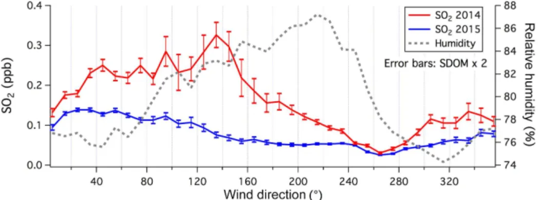
Figure 2.Averaged SO2mixing ratio and relative humidity vs. wind direction for year 2014 and 2015. Error bars on SO2indicate 2 standard errors. Elevated humidity marks the marine-influenced wind sector to be between about 60 and 260◦. Higher and more variable SO
2mixing ratios were observed from the southeast, particularly in 2014. Icelandic volcano plumes (e.g., Fig. A1) were excluded from averaging.
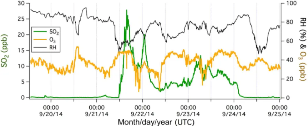
Figure 3.Example of local ship plumes on a day of southeasterly winds. Sharp peaks in SO2and CO2generally coincided with sudden depletions in O3(1 min average).
Atmospheric SO2 and humidity varied significantly at PPAO depending on wind direction (Fig. 2). Increased rel-ative humidity clearly indicates the marine-influenced wind sector from northeast to west/southwest. SO2mixing ratios were higher and more variable when the air mass had trav-eled from the southeast than when it had come from the southwest. This elevated SO2 signal was more pronounced in 2014 (averaged between May and December) than in 2015 (averaged between January and November). The lowest SO2 mixing ratios were observed in the western wind sector in both years. In the appendix, we show episodes of large SO2 plumes from the Icelandic volcano Bárdarbunga as observed at PPAO. These volcanic events do not affect our analysis of SO2in the marine atmosphere since winds were from the northwest.
3.1 Ship plumes and SO2frequency distributions
Figure 3 shows a ship plume-influenced time series during a period of southeasterly winds. Sharp spikes in SO2 coin-cided with spikes in CO2 (e.g., at about 12:00 and 15:40 UTC), which lasted for just a few minutes and likely cor-responded to local (within a few kilometers) ship emissions. O3was significantly depleted in these plumes because of its reaction with nitrogen oxides (NOx) emitted from ships. A
lower, broader hump in SO2can also be observed between about 18:30 and 20:00 UTC. This was likely due to more dis-tant ship emissions that have been diluted and mixed in the atmosphere. A concurrent increase in CO2 was not obvious during these 1.5 h. Given the high background mixing ratio of CO2(∼400 ppm), ship plumes result in much smaller (ad-ditional) signal : background ratios for CO2than for SO2. As a result, CO2emitted from point sources tends to quickly be-come indistinguishable from the background with increasing distance (i.e., greater air dilution/dispersion). In Sect. 4.2, we use the ratio between the SO2and CO2peaks to estimate the ship’s apparent FSC.
Figure 4.Histogram distributions of SO2mixing ratios in 2014(a)and 2015(b)from the southeastern and southwestern wind sectors (5 min average). Distributions are normalized to the total number of observations from the respective wind sectors.
Figure 5.Average diel cycles of SO2mixing ratio, separated into the southeastern and southwestern wind sectors for 2014(a)and 2015(b). SO2in the southwestern sector showed diel variability that is largely consistent with DMS oxidation. SO2in the southeastern sector was significantly lower and less variable in 2015 than in 2014.
for the southeastern wind sector. For example, SO2 mixing ratios from the southeast exceeded 0.5 ppb∼1 % of the time in 2015 (compared to∼11 % in 2014).
3.2 Diel variability in SO2
We compute the mean diel cycles of SO2 mixing ratio in the southeastern and the southwestern sectors for both 2014 (May to December) and 2015 (January to November), which are shown in Fig. 5. The long averaging periods help to re-duce measurement noise and also allow variability caused by horizontal transport to largely cancel. SO2 from the south-west shows a very tight diel cycle and low variability (rel-ative standard errors less than 10 %). SO2mixing ratio was the lowest near sunrise, increased throughout the day, and de-creased after sunset. This diel cycle suggests that SO2from the southwest came primarily from the photooxidation of bi-ologically derived DMS. Differences in the mean SO2diel cycles in 2014 and 2015 for the southwestern sector are largely due to the different months used in the averaging. Considering only the months of May to November, mean SO2mixing ratios in this wind sector for the 2 years differ by only∼0.01 ppb (see Sect. 4.1).
SO2 from the southeast was about 3 times higher and also more variable than from the southwest in 2014. Peaks
in SO2 were observed in the morning, mid-afternoon, and early evening. These timings are consistent with the schedule of channel-crossing ferries, which enter Plymouth Sound at least once a day from approximately due south. In 2015, SO2 from the southeast was about 2 times higher than from the southwest and variability in SO2mixing ratio was reduced. In both years, SO2 from the southeast shows an underlying diel trend (i.e., increasing during the day and decreasing at night) that suggests contributions from DMS oxidation. This implies that SO2 from the southeast is made up of at least two major components: ship emissions and DMS oxidation.
3.3 SO2from DMS oxidation
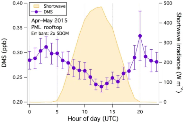
from the southwest and southeast were comparable during the 2015 measurement period (21 April to 15 May). The mean DMS diel cycle from the marine sector (Fig. 6) clearly shows an anticorrelation with shortwave irradiance, implying daytime oxidation by OH (mostly to SO2). The diel ampli-tude in DMS mixing ratio was∼0.09 ppb. A day/night differ-ence in atmospheric DMS was also observed from the PML rooftop in June 2012 from marine air (Yang et al., 2013).
The conversion efficiency from DMS to SO2 due to OH oxidation is about 70–90 % (Davis et al., 1999; Chen et al., 2000; Shon et al., 2001). At a conversion efficiency of 80 %, 0.09 ppb of oxidized DMS would lead to about 0.07 ppb of SO2 produced during the day. In comparison, over the 1.5 years of observations at PPAO the mean amplitude of the SO2 diel cycle from the southwest was∼0.06 ppb. This compar-ison is qualitative because DMS was only measured during the spring/summer periods and at a different location. Never-theless, it appears that within the measurement uncertainties DMS oxidation can account for the vast majority of the ob-served SO2diel cycle from the southwestern wind sector.
3.4 Removal of SO2from the marine atmosphere
SO2is mainly removed from the marine boundary layer via aqueous oxidation (e.g., cloud processing), deposition to the ocean, and possibly dilution by the free tropospheric air. We can approximate the total loss of SO2 from the nighttime change in the averaged SO2mixing ratio (daytime SO2 ox-idation is very slow). This calculation assumes no temporal trend in any nocturnal ship emissions (on a diel timescale) and a constant marine boundary layer height. In a polluted marine environment, a small amount of SO2could be formed at night via DMS oxidation by the nitrate radical (NO3; Yvon et al., 1996), a process we neglect here. A linear fit to the nighttime decrease of SO2from the southwest in 2014 (Fig. 5a) yields a total loss rate of about 0.2 ppb per day. The average SO2 mixing ratio was about 0.1 ppb in the evening hours, which implies a SO2residence time of approximately 0.5 d. In 2015, the total loss rate was about 0.1 ppb per day, which also implies a SO2residence time of∼0.5 d. This res-idence time is in close agreement with previous estimates in the marine atmosphere (e.g., Cuong et al., 1975; Yang et al., 2011b).
We compute the dry deposition flux of SO2to the surface ocean as−Vd·[SO2], where [SO2] is the atmospheric SO2 concentration andVdis the deposition velocity of SO2. Upon contact with seawater, SO2rapidly dissociates to form HSO−3 and then sulfite (Eigen et al., 1964). The effective solubility of SO2in seawater (pH∼8) due to this chemical enhance-ment is very large (dimensionless water : air solubility of about 5e8), which means that air–sea SO2exchange should be gas phase controlled. Oxidation to sulfate permanently re-moves sulfite from the surface ocean with a timescale of min-utes to hours (Schwartz, 1992). The combination of a low aqueousS(IV) concentration (e.g., Campanella et al., 1995;
Figure 6.Average diel variability in DMS mixing ratio and short-wave irradiance, measured from the PML rooftop between April and May 2015 (wind from the marine sector). Error bars indicate 2 standard errors.
Hayes et al., 2006) and a high effective solubility results in a near-zero interfacial SO2 concentration that is in equilib-rium with seawater (e.g., Liss and Slater, 1974). We com-pute the deposition velocity of SO2 using the COARE gas transfer model (Fairall et al., 2011), which utilizes the air-side diffusivity of SO2 from Johnson (2010) and the mea-sured wind speed at PPAO. Diel cycles in SO2 deposition flux (Fig. 7) resemble the mirror image of SO2mixing ratio. For the southwestern wind sector, the average SO2 deposi-tion flux was about−1 to−2 µmole m−2d−1.
For the southeastern sector, deposition flux averaged about −3 µmole m−2d−1in 2014 and−1 µmole m−2d−1in 2015. Interestingly, while SO2 mixing ratio from the southeast was still higher than from the southwest in 2015, deposi-tion fluxes between the two wind sectors were comparable. This is because wind speeds were typically lower from the southeast. Overall, dry deposition removes SO2from a well-mixed, 1 km deep marine atmospheric boundary layer with a timescale of∼2 days at PPAO. It accounted for approxi-mately a quarter of the total SO2losses, similar to previous findings (e.g., Yang et al., 2011b).
4 Discussion
4.1 Long-term changes in SO2and ship emissions
Figure 7.Mean diel cycles in the wind speed-dependent SO2deposition flux, separated into the southeastern and southwestern wind sectors for year 2014(a)and 2015(b). Error bars indicate 2 standard errors. SO2deposition flux was significantly greater in the southeastern sector than in the southwestern sector in 2014.
Figure 8.Monthly means and 25th/75th percentiles of SO2mixing ratio from southeastern and southwestern wind sectors. SO2from the southwest shows a clear seasonal cycle, with higher values in summer/early autumn and lower values in winter/early spring. A similar underlying seasonal variability is also apparent in SO2from the southeastern sector.
spring compared to summer/early autumn. The seasonal cy-cle in SO2from the southwest is consistent with the variabil-ity in surface seawater DMS concentration previously mea-sured at the nearby L4 mooring station (∼6 nM in summer and∼1 nM in winter; Archer et al., 2009). Using those sea-water DMS concentrations, local wind speeds and tempera-tures, and the DMS air–sea transfer velocity from Yang et al. (2011a), we predict DMS fluxes on the order of ∼10 and 3 µmole m−2d−1 for the summer and winter, respec-tively. These fluxes would be sufficient to account for the ob-served SO2burden from the southwest (∼0.10 ppb in sum-mer and ∼0.02 ppb in winter) assuming a SO2 residence time of 0.5 day in a 1 km deep marine boundary layer (∼8 and ∼2 µmole m−2d−1 of sulfur required). In addition to lower seawater DMS concentrations in winter, less incoming irradiance and shorter daylight hours in those months will also reduce the photochemical production of SO2 from at-mospheric DMS. Overall, we see that the seasonal cycle of SO2in air from the southwest can largely be explained by natural variability.
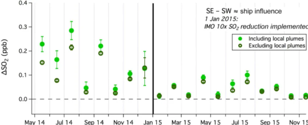
The difference in SO2mixing ratio between the southeast-ern and southwestsoutheast-ern sectors (1SO2) is shown in Fig. 9.
There is a fair amount of scatter in1SO2, which is partly because SO2measurements from the two wind sectors were not concurrent (i.e., winds could not be blowing from the southeast and southwest at any single moment). Neverthe-less, mean (±standard error)1SO2 decreased from∼0.15 (±0.03) ppb in 2014 to∼0.05 (±0.01) ppb in 2015, with a sharp drop off coincident with the 1 January 2015 mandate for ship sulfur emission reduction.
Figure 9.The difference between monthly averaged SO2mixing ratios from the southeast and southwest (1SO2), which we consider to approximately represent ship emissions.1SO2including and excluding local ship plumes is shown. Error bars are propagated from 2 times the standard errors from each wind sector. Solid vertical line indicates the 1 January 2015 mandate for reduction in ship SO2emissions.
corroborates the idea that ship emissions from the southwest only have a minor effect on our observations.
Entrainment from the free troposphere could bring anthro-pogenic SO2into the marine boundary layer (e.g., Simpson et al., 2014), which is not accounted for here. We further as-sume negligible influence of terrestrial SO2emissions (e.g., from continental Europe) in the southeastern sector because of atmospheric dilution and rapid removal of SO2from the lower atmosphere (residence time∼0.5 d, see Sect. 3.4). The English Channel near Plymouth has a width of approximately 200 km. At a speed of 5 m s−1, southeasterly winds blow over the channel in approximately half a day, comparable to the removal time.
4.2 Local ship plumes and fuel sulfur content
The SO2signals from the southeast include local ship emis-sions (e.g., from ships entering/exiting Plymouth Sound) as well as more distant emissions from the English Channel. Local emissions usually appear as sharp spikes, while more distant emissions tend to have plumes that are broader and less intense due to atmospheric dilution. We use concurrent peaks in SO2and CO2to estimate the ships’ apparent FSC. The FSC calculation assumes that all of the carbon and sul-fur in fuel is released into the atmosphere during combustion. We use the word “apparent” here because our calculation re-flects the downstream emissions rather than the actual fuel composition. Ships that “scrub” sulfur from stack emissions will have apparent FSC values that are lower than the actual FSC. To minimize the uncertainty in our estimate, we focus on well-resolved plumes from nearby ships only.
Simple dispersion modeling predicts that local ship plumes have a typical duration of a few minutes. For exam-ple, von Glasow et al. (2003) estimated the horizontal disper-sion of a ship plume as
H=H0·(t /t0)0.75. (1)
H0 andH are the horizontal extents of a plume at the ini-tial timet0(1 s) and the time of interestt. The initial plume extent (H0)is assumed to be 10 m. We estimate the horizon-tal dispersion of plumes emitted from an upwind distance of 2 km (e.g., halfway across Plymouth Sound) and 100 km (e.g., halfway across the English Channel). At a speed of 8 m s−1, wind travels 2 and 100 km in∼4 and 200 min, re-spectively. Applying these timescales to Eq. (1) yields hor-izontal plume extents of 600 and 11 000 m. For a ship 2 km away that is traversing perpendicular to the mean wind at a speed of 4 m s−1, its emission should be observable at PPAO for 2.5 min. A ship 100 km away would have a plume that is theoretically observable for nearly an hour. These timescales are roughly consistent with our time series observations (e.g., Fig. 3). Ships that do not travel perpendicular to the wind will have plumes that are observable for longer periods. Faster wind speeds or ship speeds shorten the duration of plume de-tection, and vice versa.
The following steps were used to separate local ship emis-sions from the background or more distant emisemis-sions based on 1 min average gas mixing ratios. All data processing was done with Igor Pro (WaveMetrics).
1. Apply 2 h running-median smoothing to the SO2 time series.
2. Identify “no plume” times as when the 1 min average SO2 was within 0.1 ppb (i.e., < twice the instrument noise) of the smoothed SO2.
3. Subtract the linear interpolation of the “no plume” SO2 time series from the 1 min average SO2time series to derive the SO2deviations from the background (SO′2). 4. Apply the “FindPeak” function to SO′
was 1.35 ppb in 2014 and 0.48 ppb in 2015, with a typical plume duration of∼3 min.
CO2plumes from local ship emissions were identified in an analogous fashion based on an analysis of the 1 min aver-age CO2time series (i.e., independent of the SO2analysis). The “no plume” CO2threshold (step 2 above) was set to be 0.2 ppm, and the minimum peak height required for positive peak identification (step 4) was set to be 1.0 ppm. Based on these schemes, a total number of 1242 separate CO2plumes were identified from May 2014 to November 2015, with a mean plume height of 2.6 ppm.
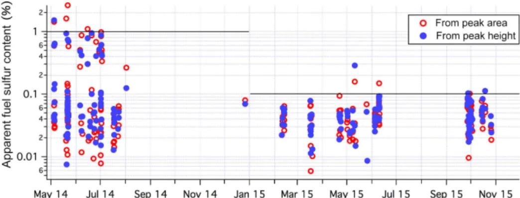
Apparent FSC is computed from coincidental SO2 and CO2 plume heights as well as plume areas (N=245) fol-lowing Kattner et al. (2015). To account for clock drift be-tween the computers that recorded the SO2 and CO2 data, we allowed the times of the SO2and CO2peaks to differ by up to 1 min. The results of these calculations for the marine wind sector are shown in Fig. 10. Gaps in observations were largely due to the CO2analyzer malfunctioning or winds out of sector. The peak area and peak height methods yielded similar results. FSC from peak area appears to be slightly more variable, possibly due to a greater sensitivity toward the definition of plume baseline. Based on peak height, in 2014 the mean (±standard error) FSC was 0.17 (±0.03) %, with ∼99 % of the plumes below the IMO threshold of 1 % FSC. About 70 % of the plumes were already below 0.1 % FSC in 2014. In 2015, mean FSC decreased to 0.047 (±0.003) %, with ∼99 % of the plumes below the new IMO threshold of 0.1 %. FSC estimated from the peak area method shows slightly lower levels of compliance (∼95 % for both years). The reduction in mean FSC from 2014 to 2015 is propor-tionally comparable to the decrease in 1SO2 computed in Sect. 4.1.
Our FSC estimates illustrate a fairly similar decreasing trend to that observed near the Hamburg harbor (Kattner et al., 2015). The mean FSC value at PPAO is approximately half of what was estimated by Kattner et al. (2015) for the year 2014 and is comparable to their estimate for 2015. How-ever, our observations are different in several aspects. The vast majority of the ships entering/leaving Plymouth Sound are naval, commercial ferries, and private vessels according to the Devonport Naval Base Ship Movement Report. The number of large container ships entering Plymouth Sound is proportionally much lower than near Hamburg. Because the distances between ships and PPAO were not fixed (as op-posed to spatially restricted sampling locations in Kattner
SO2and CO2measurements. A higher SO2spike threshold could bias our FSC estimates towards plumes with greater sulfur content, while a lower threshold would be too close to the noise level of the measurement. Long-term records of another tracer (e.g., nitrogen oxides or black carbon) would allow for a more independent identification of ship plumes for the calculation of FSC. Finally, we reiterate that our FSC estimates are for well-resolved peaks from local ship plumes, which do not necessarily reflect ship emissions from the main shipping lanes of the English Channel.
4.3 Top-down estimates of SO2emissions from the
English Channel
We use1SO2with local ship emissions excluded (Fig. 9) to estimate distant anthropogenic SO2emissions (e.g., from the English Channel). Without local spikes (i.e., the “no plume” SO2time series in Sect. 4.2), the computed mean SO2mixing ratio from the southwest is only slightly lower, as might be expected due to the relatively low ship density in that direc-tion; in contrast, mean SO2mixing ratio from the southeast is lowered by∼0.04 ppb in 2014 and∼0.01 ppb in 2015. Ap-proximately a quarter of the SO2attributed to ship emissions in Sect. 4.1 (1SO2)was due to local ship plumes.1SO2 ex-cluding local ship emissions was∼0.11 (±0.03) ppb in 2014 and∼0.04 (±0.01) ppb in 2015. The largest differences in
1SO2with and without nearby plumes occurred in the sum-mer for both years, when the ship traffic was the heaviest.
We make an order of magnitude estimate for the ship emissions in the English Channel required to sustain the ob-served SO2 mixing ratios. This calculation assumes a SO2 residence time of 0.5 d in a well-mixed, 1 km deep marine atmospheric boundary layer. For this scenario it would take ∼9 µmole m−2d−1of SO2from ships to account for a1SO2 of 0.11 ppb and∼3 µmole m−2d−1 of SO2 emission from ships to account for a 1SO2 of 0.04 ppb. Simplistic ex-trapolation of these fluxes to the area of the English Chan-nel (about 75 000 km2)yields a total ship SO
Figure 10.Apparent fuel sulfur content (FSC) estimated from peak areas as well as peak heights of coincidental SO2and CO2plumes (1 min averaged data). Solid horizontal lines indicate IMO fuel sulfur emission content limits in European waters (SECA) regions: 1 % SFC in 2014 and 0.1 % SFC in 2015.
Our SO2emission estimate is low in part because we have purposely excluded local ship plumes. Also,1SO2could be a slight underestimate of ship emissions due to the assump-tion of zero ship influence in the southwestern wind sector. More accurate constraints of sulfur emissions from the En-glish Channel from point measurements such as at PPAO probably require modeling of air trajectory/dispersion, de-tailed information about ship traffic, and knowledge of the SO2source area (i.e., the concentration footprint; Wilson and Swaters, 1991; Schmid, 1994). A more complete description of the sulfur budget in this environment would also require sulfate concentration measurements in aerosols as well as in precipitation droplets.
5 Conclusions
Figure A1.Very high SO2mixing ratios were observed in Icelandic volcano plumes. Elevated SO2sometimes coincided with increased O3 and reduced relative humidity (RH), consistent with entrainment from the free troposphere.
Appendix A: SO2from volcanic eruption
Acknowledgements. Trinity House (http://www.trinityhouse.co. uk/) owns the Penlee site and has kindly agreed to lease the building to PML so that the instruments can be protected from the elements. We are able to access the site thanks to the cooperation of Mount Edgcumbe Estate (http://www.mountedgcumbe.gov.uk/). Thanks to S. Atkinson and M. Sillett (Plymouth University) for routine maintenance of site, S. Ussher (Plymouth University), P. Agnew, N. Savage, and L. Neal (UK Met Office) for valuable scientific discussions, R. Pascal and M. Yelland (National Oceanography Centre, Southampton) for letting us deploy the Picarro instrument, and B. Carlton (Plymouth Marine Laboratory) for setting up data communication. We also thank the reviewers for their constructive comments and suggestions. T. Bell and M. Yang dedicate this publication to the late Roland von Glasow, who was a source of great inspiration and support to us both.
Edited by: E. Harris
References
Agrawal, H., Malloy, Q. G. J., Welch, W. A., Wayne Miller, J., and Cocker III, D. R.: In-use Gaseous and Particulate Matter Emis-sions from a Modern Ocean Going Container Vessel, Atmos. Environ., 42, 5504–5510, doi:10.1016/j.atmosenv.2008.02.053, 2008.
Archer, S. D., Cummings, D. G., Llewellyn, C. A., and Fishwick, J. R.: Phytoplankton taxa, irradiance and nutrient availability deter-mine the seasonal cycle of DMSP in temperate shelf seas, Mar. Ecol. Prog. Ser., 394, 111–124, doi:10.3354/meps08284, 2009. Aulinger, A., Matthias, V., Zeretzke, M., Bieser, J., Quante, M., and
Backes, A.: The impact of shipping emissions on air pollution in the greater North Sea region – Part 1: Current emissions and con-centrations, Atmos. Chem. Phys., 16, 739–758, doi:10.5194/acp-16-739-2016, 2016.
Bandy, A. R., Thornton, D. C., Blomquist, B. W., Chen, S., Wade, T. P., Ianni, J. C., Mitchell, G. M., and Nadler, W.: Chemistry of dimethyl sulfide in the equatorial Pacific atmosphere, Geophys. Res. Lett., 23, 741–744, 1996.
Beecken, J., Mellqvist, J., Salo, K., Ekholm, J., Jalkanen, J.-P., Jo-hansson, L., Litvinenko, V., Volodin, K., and Frank-Kamenetsky, D. A.: Emission factors of SO2, NOx and particles from ships in Neva Bay from ground-based and helicopter-borne measure-ments and AIS-based modeling, Atmos. Chem. Phys., 15, 5229– 5241, doi:10.5194/acp-15-5229-2015, 2015.
Campanella, L., Cipriani, P., Martini, T. M., Sammartino, M. P., and Tomassetti, M.: New enzyme sensor for sulfite analysis in sea and river water samples, Anal. Chim. Acta, 305, 32–41, 1995. Capaldo, K., Corbett, J. J., Kasibhatla, P., Fischbeck, P. S., and
Pan-dis, S. N.: Effects of ship emissions on sulphur cycling and radia-tive climate forcing over the ocean, Nature, 400, 743–746, 1999. Charlson, R. J. and Rodhe, H.: Factors controlling the acidity of
rainwater, Nature, 295, 683–685, 1982.
Charlson, R. J., Lovelock, J. E., Andreae, M. O., and Warren S. G.: Oceanic phytoplankton, atmospheric sulfur, cloud albedo and climate, Nature, 326, 655–661, 1987.
Clarke, A. D., Davis, D., Kapustin, V. N., Eisele, F., Chen, G., Paluch, I., Lenschow, D., Bandy, A. R., Thornton, D., Moore, K., Mauldin, L., Tanner, D., Litchy, M., Carroll, M. A., Collins,
J., and Albercook, G.: Particle nucleation in the tropical bound-ary layer and its coupling to marine sulfur sources, Science, 282, 89–92, 1998.
Chen, G., Davis, D. D., Kasibhatla, P., Bandy, A. R., Thornton D. C., Huebert, B. J., Clarke, A. D., and Blomquist, B. W.: A study of DMS oxidation in the tropics: comparison of Christmas Island field observations of DMS, SO2, and DMSO with model simula-tions, J. Atmos. Chem., 37, 137–160, 2000.
Collins, W. J., Sanderson, M. G., and Johnson, C. E.: Impact of increasing ship emissions on air quality and deposition over Europe by 2030, Meteorologische Z., doi:10.1127/0941-2948/2008/0296, published online, 2008.
Corbett, J. J., Winebrake, J. J., Green, E. H., Kasibhatla, P., Eyring, V., and Lauer, A.: Mortality from Ship Emissions: A Global Assessment, Environ. Sci. Technol., 41, doi:10.1021/es071686z, 8512–8518, 2007.
Cuong, N, B. C., Bonsang, B., Lambert, G., and Pasquier, J. L. Residence time of sulfur dioxide in the marine atmosphere, Pure Appl. Geophys., 123, 489–500, 1975.
Dalsøren, S. B., Eide, M. S., Endresen, Ø., Mjelde, A., Gravir, G., and Isaksen, I. S. A.: Update on emissions and environmental im-pacts from the international fleet of ships: the contribution from major ship types and ports, Atmos. Chem. Phys., 9, 2171–2194, doi:10.5194/acp-9-2171-2009, 2009.
Davis, D., Chen, G., Bandy, A., Thornton D., Eisele, F., Mauldin, L., Tanner, D., Lenschow, D., Fuelberg, H., Huebert B., Heath, J., Clarke, A., and Blake, D.: Dimethylsulfide oxidation in the equatorial Pacific: comparison of model simulations with field observations for DMS, SO2, H2SO4(g), MSA(g), MS, and NSS, J. Geophys. Res., 104, 5765–5784, 1999.
Eigen, M., Kruse, W., Maass, G., and De Maeyer, L.: Rate constants of protolytic reactions in aqueous solution, in: Progress in Reac-tion Kinetics, Vol. 2, edited by: Porter, G., 285–318, Pergamon, Oxford, 1964.
Endresen, Ø., Sørgård, E., Sundet, J. K., Dalsøren, S. B., Isaksen, I. S. A., Berglen, T. F., and Gravir, G.: Emission from international sea transportation and environmental impact, J. Geophys. Res., 108, 4560, doi:10.1029/2002JD002898, 2003.
Eyring, V., Koehler, H. W., van Aardenne, J., and Lauer, A.: Emis-sions from international shipping: 1. The last 50 years, J. Geo-phys. Res., 110, D17305, doi:10.1029/2004JD005619, 2005a. Eyring, V., Köhler, H. W., Lauer, A., and Lemper, B.:
Emis-sions from international shipping: 2. Impact of future technolo-gies on scenarios until 2050, J. Geophys. Res., 110, D17306, doi:10.1029/2004JD005620, 2005b.
Fairall, C. W., Yang, M., Bariteau, L., Edson, J. B., Helmig, D., McGillis, W., Pezoa, S., Hare, J. E., Huebert, B., and Blomquist, B.: Implementation of the Coupled Ocean-Atmosphere Response Experiment flux algorithm with CO2, dimethyl sulfide, and O3, J. Geophys. Res., 116, C00F09, doi:10.1029/2010JC006884, 2011. Hayes, M., Taylor, G., Aster, Y. M., and Scranton, M. J.: Vertical distributions of thiosulfate and sulfite in the Cariaco Basin, Limnol. Oceanogr. 01/2006, 51, 280–287, doi:10.4319/lo.2006.51.1.0280, 2006.
Hegg, D. A.: The importance of liquid-phase oxidation of SO2in the troposphere, J. Geophys. Res., 20, 3773–3779, 1985. Jalkanen, J.-P., Johansson, L., and Kukkonen, J.: A comprehensive
Liss, P. S. and Slater, P. G.: Flux of Gases across the air-sea inter-face, Nature, 247, 181–184, 1974.
Lynch, J. A., Bowersox, V. C., and Grimm, J. W.: Changes in sulfate deposition in eastern USA following implementation of Phase I of Title IV of the Clean Air Act Amendments of 1990, Atmos. Environ., 34, 1665–1680, 2000.
Malm, W. C., Schichtel, B. A., Ames, R. B., and Gebhart, K. A.: A 10-year spatial and temporal trend of sulfate across the United States, J. Geophys. Res., 107, 4627, doi:10.1029/2002JD002107, 2002.
Matthias, V., Bewersdorff, I., Aulinger, A., and Quante, M.: The contribution of ship emissions to air pollution in the North Sea regions, Environ. Pollut., 158, 2241–2250, 2010.
Schmid, H. P.: Source areas for scalars and scalar fluxes, Bound. Lay. Meteorol., 67, 293–318, 1994.
Schwartz, S. E.: Factors governing dry deposition of gases to sur-face water, in: Precipitation Scavenging and Atmosphere-Sursur-face Exchange, edited by: Schwartz, S. E. and Slinn, W. G. N., Vol-ume ii, Hemisphere Publishing Corp, Washington, 1992. Shon, Z. H., Davis, D., Chen, G., Grodzinsky, G., Bandy, A.,
Thorn-ton, D., Sandholm, S., Bradshaw, J., Stickel, R., Chameides, W., Kok, G., Russell, L., Mauldin, L., Tanner, D., and Eisele, F.: Evaluation of the DMS flux and its conversion to SO2over the southern ocean, Atmos. Environ., 35, 159–172, 2001.
Simpson, R. M. C., Howell, S. G., Blomquist, B. W., Clarke, A. D., and Huebert, B. J.: Dimethyl sulfide: Less important than long-range transport as a source of sulfate to the remote tropi-cal Pacific marine boundary layer, J. Geophys. Res.-Atmos., 119, 9142–9167, doi:10.1002/2014JD021643, 2014.
Vestreng, V., Myhre, G., Fagerli, H., Reis, S., and Tarrasón, L.: Twenty-five years of continuous sulphur dioxide emis-sion reduction in Europe, Atmos. Chem. Phys., 7, 3663–3681, doi:10.5194/acp-7-3663-2007, 2007.
von Glasow, R., Lawrence, M. G., Sander, R., and Crutzen, P. J.: Modeling the chemical effects of ship exhaust in the cloud-free marine boundary layer, Atmos. Chem. Phys., 3, 233–250, doi:10.5194/acp-3-233-2003, 2003.
Whall, C., Scarborough, T., Stavrakaki, A., Green, C., Squire, J., and Noden, R.: UK Ship Emissions In-ventory, Entec UK Ltd, London, UK, available at: http://uk-air.defra.gov.uk/assets/documents/reports/cat15/ 1012131459_21897_Final_Report_291110.pdf (last access: January 2010), 2010.
marine boundary layer from sea-to-air eddy covariance flux mea-surements of dimethylsulfide, Atmos. Chem. Phys., 9, 9225– 9236, doi:10.5194/acp-9-9225-2009, 2009.
Yang, M., Blomquist, B. W., Fairall, C. W., Archer, S. D., and Hue-bert, B. J.: Air-sea exchange of dimethylsulfide in the South-ern Ocean: Measurements from SO GasEx compared to tem-perate and tropical regions, J. Geophys. Res., 116, C00F05, doi:10.1029/2010JC006526, 2011a.
Yang, M., Huebert, B. J., Blomquist, B. W., Howell, S. G., Shank, L. M., McNaughton, C. S., Clarke, A. D., Hawkins, L. N., Rus-sell, L. M., Covert, D. S., Coffman, D. J., Bates, T. S., Quinn, P. K., Zagorac, N., Bandy, A. R., de Szoeke, S. P., Zuidema, P. D., Tucker, S. C., Brewer, W. A., Benedict, K. B., and Collett, J. L.: Atmospheric sulfur cycling in the southeastern Pacific – longitudinal distribution, vertical profile, and diel variability ob-served during VOCALS-REx, Atmos. Chem. Phys., 11, 5079– 5097, doi:10.5194/acp-11-5079-2011, 2011b.
Yang, M., Beale, R., Smyth, T., and Blomquist, B.: Measurements of OVOC fluxes by eddy covariance using a proton-transfer-reaction mass spectrometer – method development at a coastal site, Atmos. Chem. Phys., 13, 6165–6184, doi:10.5194/acp-13-6165-2013, 2013.
Yang, M., Bell, T. G., Hopkins, F. E., Kitidis, V., Cazenave, P. W., Nightingale, P. D., Yelland, M. J., Pascal, R. W., Prytherch, J., Brooks, I. M., and Smyth, T. J.: Air-Sea Fluxes of CO2 and CH4 from the Penlee Point Atmospheric Observatory on the South West Coast of the UK, Atmos. Chem. Phys. Discuss., doi:10.5194/acp-2015-717, in review, 2016.
Yvon, S. A., Plane, J. M. C., Nien, C.-F., Cooper, D. J., and Saltz-man, E. S.: The interaction between the nitrogen and sulfur cy-cles in the polluted marine boundary layer, J. Geophys. Res., 101, 1379–1386, 1996.