ACPD
10, 16111–16151, 2010Anthropogenic sulfur dioxide emissions:
1850–2005
S. J. Smith et al.
Title Page
Abstract Introduction
Conclusions References
Tables Figures
◭ ◮
◭ ◮
Back Close
Full Screen / Esc
Printer-friendly Version Interactive Discussion
Discussion
P
a
per
|
Dis
cussion
P
a
per
|
Discussion
P
a
per
|
Discussio
n
P
a
per
|
Atmos. Chem. Phys. Discuss., 10, 16111–16151, 2010 www.atmos-chem-phys-discuss.net/10/16111/2010/ doi:10.5194/acpd-10-16111-2010
© Author(s) 2010. CC Attribution 3.0 License.
Atmospheric Chemistry and Physics Discussions
This discussion paper is/has been under review for the journal Atmospheric Chemistry and Physics (ACP). Please refer to the corresponding final paper in ACP if available.
Anthropogenic sulfur dioxide emissions:
1850–2005
S. J. Smith1, J. van Aardenne2,*, Z. Klimont2, R. Andres3, A. Volke1, and S. Delgado Arias1
1
Joint Global Change Research Institute, Pacific Northwest National Laboratory, 5825 University Research Court, Suite 3500, College Park, MD 20740, USA
2
European Commission Joint Research Centre, European Commission, Via E. Fermi 2749, TP 290,I – 21027 Ispra (VA), Italy
3
Oak Ridge National Laboratory, P.O. Box 2008, Oak Ridge, TN 37831, USA
*
current address: European Environment Agency, Kongens Nytorv 6, 1050 Copenhagen, Denmark
Received: 28 May 2010 – Accepted: 7 June 2010 – Published: 30 June 2010
Correspondence to: S. J. Smith ([email protected])
ACPD
10, 16111–16151, 2010Anthropogenic sulfur dioxide emissions:
1850–2005
S. J. Smith et al.
Title Page
Abstract Introduction
Conclusions References
Tables Figures
◭ ◮
◭ ◮
Back Close
Full Screen / Esc
Printer-friendly Version Interactive Discussion
Discussion
P
a
per
|
Dis
cussion
P
a
per
|
Discussion
P
a
per
|
Discussio
n
P
a
per
|
Abstract
Sulfur aerosols impact human health, ecosystems, agriculture, and global and regional climate. A new annual estimate of anthropogenic global and regional sulfur dioxide emissions has been constructed spanning the period 1850–2005 using a bottom-up mass balance method, calibrated to country-level inventory data. Global emissions
5
peaked in the early 1970s and decreased until 2000, with an increase in recent years due to increased emissions in China, international shipping, and developing countries in general. An uncertainty analysis was conducted including both random and systemic uncertainties. The overall global uncertainty in sulfur dioxide emissions is relatively small, but regional uncertainties ranged up to 30%. The largest contributors to
uncer-10
tainty at present are emissions from China and international shipping. Emissions were
distributed on a 0.5◦grid by sector for use in coordinated climate model experiments.
1 Introduction
Anthropogenic emissions have resulted in greatly increased sulfur deposition and at-mospheric sulfate loadings near most industrialized areas. Sulfate acid deposition can
15
be detrimental to ecosystems, harming aquatic animals and plants, and damaging to a wide range of terrestrial plant life. Sulfur dioxide forms sulfate aerosols that are
thought to have a significant effect on global and regional climate. Sulfate aerosols
reflect sunlight into space and also act as condensation nuclei, which tend to make clouds more reflective and change their lifetimes. The radiative forcing change wrought
20
by sulfate aerosols may be second only to that caused by carbon dioxide, albeit in the opposite direction (Forster et al., 2007).
Sulfur is ubiquitous in the biosphere and often occurs in relatively high concentra-tions in fossil fuels, with coal and crude oil deposits commonly containing 1–2% sulfur by weight. The widespread combustion of fossil fuels has, therefore, greatly increased
25
substan-ACPD
10, 16111–16151, 2010Anthropogenic sulfur dioxide emissions:
1850–2005
S. J. Smith et al.
Title Page
Abstract Introduction
Conclusions References
Tables Figures
◭ ◮
◭ ◮
Back Close
Full Screen / Esc
Printer-friendly Version Interactive Discussion
Discussion
P
a
per
|
Dis
cussion
P
a
per
|
Discussion
P
a
per
|
Discussio
n
P
a
per
|
tially greater than natural emissions on a global basis (Smith et al., 2001).
Historical reconstructions of sulfur dioxide emissions are necessary to access the past influence of sulfur dioxide on the earth system and as base-year information for future projections (Lamarque et al., 2010). This paper presents a new estimate of global and regional sulfur dioxide anthropogenic emissions over the period from 1850
5
to 2005. This work represents a substantial update of previous work (Smith et al., 2001; Smith et al., 2004) with newer data and improved methodologies. The
emis-sions reconstruction presented here accounts for regional differences in the pace and
extent of emission control programs, has annual resolution, includes all anthropogenic sources, and provides global coverage. Fuel-based and activity-based (Eyring et al.,
10
2009) estimates of shipping emissions were reconciled for recent decades and then extrapolated to 1850. A global mass balance for sulfur in crude oil was calculated as an independent estimate of petroleum emissions. Finally, a regional and global uncer-tainty analysis was conducted.
2 Methodology
15
Sulfur emissions from combustion and metal smelting can, in principle, be estimated using a bottom-up mass balance approach where emissions are equal to the sulfur content of the fuel (or ore) minus the amount of sulfur removed or retained in bottom ash or in products. Data limitations, however, make the bottom-up approach uncer-tain. Countries with air pollution policies in place generally require detailed reporting of
20
emissions, including direct measurement of emissions for many large sources. These data are likely to be more accurate than bottom-up estimates; therefore, we constrain our calculations to match country-level inventories where these data are available and judged to be reliable. This method produces an emissions estimate that is consistent with the available country inventory data, contains complete coverage of all relevant
25
ACPD
10, 16111–16151, 2010Anthropogenic sulfur dioxide emissions:
1850–2005
S. J. Smith et al.
Title Page
Abstract Introduction
Conclusions References
Tables Figures
◭ ◮
◭ ◮
Back Close
Full Screen / Esc
Printer-friendly Version Interactive Discussion
Discussion
P
a
per
|
Dis
cussion
P
a
per
|
Discussion
P
a
per
|
Discussio
n
P
a
per
|
Emissions were estimated annually by country for the following sectors: coal com-bustion, petroleum comcom-bustion, biomass comcom-bustion, shipping bunker fuels, metal smelting, natural gas processing and combustion, petroleum processing, pulp and pa-per processing, other industrial processes, and agricultural waste burning (AWB). The approach was to first develop a detailed inventory estimate by sector and country for
5
three key years: 1990, 2000, and 2005. These years were chosen due to data avail-ability and because these years span a time period of significant change in emissions controls. Estimates for other years were constructed by interpolating emissions factors, while calibrating to country-level emissions inventories where those were available.
These sectoral emissions were then transformed to a set of standard reporting
sec-10
tors (energy, industry, transportation, domestic, AWB) before downscaling to a 0.5◦
spatial grid. Descriptions of each element in this calculation are given below, with further details in the supplementary material.
2.1 Fossil fuel combustion
Emissions from coal and petroleum combustion were estimated starting with the
re-15
gional emissions factors from Smith et al. (2001). A composite fossil fuel consumption time series was constructed (see supplementary material) using data from IEA (2006), UN energy statistics (1996), and Andres et al. (1999), who compiled historical esti-mates from Etemad et al. (1991). Country-level emissions estiesti-mates for Europe, North America, Japan, Australia, and New Zealand were compiled from: UNFCCC (2009)
20
for 1990–2005; Environment Canada (2008), the EEA (2002), Fujita (1993), Mylona (1996), Gschwandtner et al. (1986), UK National Atmospheric Emissions Inventory (2009), USEPA (1996a), and Vestreng et al. (2007) as detailed in the supplementary material. Fossil-fuel emissions factors were adjusted such that total emissions matched inventory values for those years where inventory values are available.
25
ACPD
10, 16111–16151, 2010Anthropogenic sulfur dioxide emissions:
1850–2005
S. J. Smith et al.
Title Page
Abstract Introduction
Conclusions References
Tables Figures
◭ ◮
◭ ◮
Back Close
Full Screen / Esc
Printer-friendly Version Interactive Discussion
Discussion
P
a
per
|
Dis
cussion
P
a
per
|
Discussion
P
a
per
|
Discussio
n
P
a
per
|
Mylona (1996), we linearly increased the assumed sulfur retained in ash for coal com-bustion to 20% in 1920, starting from regional values in 1960, to account for changing coal combustion technologies. Coal used for the production of coke or as process heat for cement manufacture is not included in the calculation of combustion emissions in recent years; any residual emissions from these uses are assumed to be included in
5
the process emissions estimate. Emissions from coal used for coke production are included in earlier years before the introduction of by-product coke plants (see sup-plementary material). The assumptions for sulfur emissions from coal combustion in China and the countries of the Former Soviet Union are drawn from (Foell et al., 1995; Klimont et al., 2009; Xu et al., 2009) and (Ryaboshapko et al., 1996), respectively as
10
discussed in the supplementary material. The sulfur content of coal within each country is assumed to be constant over time except as indicated above. This assumption can be problematic for countries with significant imports unless detailed country-level in-ventory data are available. To examine the potential importance of this assumption, we examined coal imports and emissions in 1990 (the situation is similar in 2005). There
15
were only three countries outside of Europe and Japan, where we have calibrated to emission inventories, with imports larger than 10 000 tonnes per year: Brazil, South Korea, and Taiwan. While there are other countries with large net coal imports relative to consumption, the fraction of sulfur emissions from coal in those countries is small.
We estimate coal to have produced 11%, 25%, and 24% of SO2 emissions in these
20
three countries in 1990. Information on the source of coal imports over time would be helpful to refine emissions estimates from these countries, although the impact is relatively small in absolute terms. A more refined estimate is complicated by the need to know not only the properties of imported coal but also its use. For example, the
emissions impact of coal used to produce coal coke can be very different than coal
25
used for electricity generation.
ACPD
10, 16111–16151, 2010Anthropogenic sulfur dioxide emissions:
1850–2005
S. J. Smith et al.
Title Page
Abstract Introduction
Conclusions References
Tables Figures
◭ ◮
◭ ◮
Back Close
Full Screen / Esc
Printer-friendly Version Interactive Discussion
Discussion
P
a
per
|
Dis
cussion
P
a
per
|
Discussion
P
a
per
|
Discussio
n
P
a
per
|
(see supplementary material). These estimates differ from each other in some
coun-tries and sectors, highlighting a need for improved inventories in this rapidly changing region.
Petroleum emissions are particularly difficult to estimate in the absence of detailed,
country-level inventory data. For regions without detailed emission inventory data,
de-5
fault values for sulfur contents were used. Emissions factors were adjusted downward in recent years to account for increased stringency of sulfur content standards as re-ported in UNEP (2008).
As an overall check on the petroleum assumptions used, a global petroleum mass balance was constructed by calculating the total amount of sulfur in crude oil and
sub-10
tracting the amount of sulfur removed in refineries (see supplemental information). The final mass balance estimate for global sulfur emissions from petroleum as compared to the inventory estimate is shown in Fig. 1 for the period 1950–2005, where petroleum emissions are a substantial fraction of the global total. We estimate that in the early portion of the 21st century the world passed a threshold where slightly over half of
15
the sulfur contained in crude oil is removed at the refinery. Thus, global emissions from petroleum have been relatively flat since 1985 despite increases in petroleum consumption. Mass balance estimates using two assumptions for the amount of sulfur that is retained in non-energy use of petroleum products and non-combusted products, such as asphalt, are shown in order to reflect uncertainty in this parameter.
20
The resulting estimate of global petroleum sulfur is consistent with the global inven-tory value for petroleum emissions for most years. The mass-balance estimate
indi-cates that there may be an underestimate on the order of 5000 Gg SO2in the inventory
data during the late 1970s. The 10% retention mass-balance case results in a lower global estimate than the inventory data past 1990. The 5% retention case matches
25
well with the inventory during this time, perhaps indicating the impact of increased
refinery efficiency. While this comparison validates the overall approach, significant
errors could still be present at the country level.
prod-ACPD
10, 16111–16151, 2010Anthropogenic sulfur dioxide emissions:
1850–2005
S. J. Smith et al.
Title Page
Abstract Introduction
Conclusions References
Tables Figures
◭ ◮
◭ ◮
Back Close
Full Screen / Esc
Printer-friendly Version Interactive Discussion
Discussion
P
a
per
|
Dis
cussion
P
a
per
|
Discussion
P
a
per
|
Discussio
n
P
a
per
|
ucts in the US as implied by current estimates (Gschwandtner et al., 1986; USEPA, 1996a) before about 1980 appeared to be lower than those for other world regions. In order to better estimate petroleum-related emissions in the United States, a mass balance estimate for the United States was constructed, accounting for imports and ex-ports of crude oil by region and imex-ports and exex-ports of petroleum products (EIA 2009).
5
This mass balance indicated that sulfur emissions from petroleum were substantially underestimated prior to 1980 by 30–50% (see Supplimentary material). The increased emissions are, in part, due to imports of residual fuel, and a decrease prior to 1980
in reported bunker fuel use, which is, in effect, an export of sulfur from the continental
areas. Emissions from petroleum prior to 1980 were increased to be within 20% of
10
the total sulfur as indicated in the mass balance estimate, allowing, conservatively, for retention of sulfur in non-combustion uses.
As a check of the assumptions used in the crude oil mass balance calculations, we compared the aggregate sulfur content of crude oil refined in the United States as es-timated by this mass-balance estimate with reported values. The estimate constructed
15
here for the mass balance calculation averages 7% higher than the average sulfur con-tent of crude input to refineries as reported by EIA from 1981–2002, and within 1% of the value reported by Bingham et al. (1973) for 1970. This lends confidence to our conclusion that emissions from petroleum combustion in the United States were underestimated in earlier years.
20
2.2 International shipping
Emissions from international shipping were estimated using a combination of reported data and bottom-up estimates of shipping fuel consumption. We constructed a com-posite global estimate of shipping fuel consumption following Eyring et al. (2009) by using values from Eyring et al. (2009) for 1896–2007 and Endresen et al. (2007) from
25
es-ACPD
10, 16111–16151, 2010Anthropogenic sulfur dioxide emissions:
1850–2005
S. J. Smith et al.
Title Page
Abstract Introduction
Conclusions References
Tables Figures
◭ ◮
◭ ◮
Back Close
Full Screen / Esc
Printer-friendly Version Interactive Discussion
Discussion
P
a
per
|
Dis
cussion
P
a
per
|
Discussion
P
a
per
|
Discussio
n
P
a
per
|
timated by combining data reported in Endresen et al. (2007) and Fletcher (1997). Values were linearly interpolated for years where no data were available. Estimates of fuel consumption for 1860 and 1850 were obtained by scaling with total ship tonnage as reported in Mitchell (1998a, b, c), using the tabulation of Bond et al. (2007).
In order to estimate sulfur emissions, we require a time series of bunker fuel
con-5
sumption by fuel type (e.g., coal, residual, distillate, and other). We estimated these data by combining reported bunker fuel sales from EIA International Energy Annual (EIA 2008, and previous years) with UN data for earlier years. These data represent reported bunker fuel sales. The bottom-up global fuel estimates above also include domestic shipping fuel consumption, so in order to produce a consistent comparison
10
we added reported values from IEA for domestic shipping and fishing (available from
1971 forward) to our composite consumption time series. The difference between the
bottom-up consumption time series and the composite reported fuel consumption time
series is remarkably small. The 5-year running average difference between the total
regional time series and the global estimate is 10% or less over the period 1971–2005.
15
We find, therefore, that reported fuel consumption over this period appears to be only slightly lower than that inferred by bottom-up analysis. Thus, we used the composite-derived fuel consumption time series as the basis for determining the split between residual and distillate fuel consumption for purposes of estimating sulfur emissions. The fraction of residual fuel used in shipping has fallen steadily over time, from an
20
estimated value of 78% in 1971 to 59% in 2005. This has a substantial impact on emissions as the sulfur content of residual oil can be much higher than that of distillate fuels. The residual fraction is kept constant prior to 1971 due to a lack of data.
These are global values for fuel consumption, which would ideally need to be rec-onciled with regional energy data. As noted by Eyring et al. (2009) for 1896–2007
25
ACPD
10, 16111–16151, 2010Anthropogenic sulfur dioxide emissions:
1850–2005
S. J. Smith et al.
Title Page
Abstract Introduction
Conclusions References
Tables Figures
◭ ◮
◭ ◮
Back Close
Full Screen / Esc
Printer-friendly Version Interactive Discussion
Discussion
P
a
per
|
Dis
cussion
P
a
per
|
Discussion
P
a
per
|
Discussio
n
P
a
per
|
consumption category in the IEA data that is large enough to include the difference
between our regional fuel consumption estimate and the IEA reported bunker fuel use.
We presume, therefore, that the difference is unreported consumption and no
adjust-ment to the IEA consumption data has been made.
In order to estimate sulfur dioxide emissions, we calibrate to the year 2000 value
5
from Eyring et al. (2009) of 11 080 kt SO2/year. Using the global division between fuels
derived above, we match this value using the following sulfur contents: residual: 2.86% and distillate: 1.25%. Further, the average value for sulfur in bunker coal is assumed to be 1.1%. For simplicity these values are kept constant over time. This is a significant source of uncertainty in international shipping emissions, which is considered further
10
in Sect. 4.
The fossil fuel consumption data from IEA used to estimate combustion emissions (Sect. 2.1) were processed to exclude fuels reported as international bunkers but in-cluded fuels used for domestic shipping and fishing, using sectoral definitions as dis-cussed further in Sect. 2.5. In parallel with this assumption, domestic shipping and
15
fishing emissions in the inventory data were included in the surface transportation sec-tor. Emissions due to domestic shipping and fishing emissions from inventory data were subtracted from the total shipping estimate in the tables and figures reported below to avoid double counting.
2.3 Metal smelting
20
Smelting emissions were estimated using a mass balance approach where emissions are equal to the gross sulfur content of ore minus reported smelter sulfuric acid pro-duction, with estimates adjusted to match inventory data where available (see supple-mentary material). Smelter production of copper, zinc, lead, and nickel was tabulated by country, primarily using USGS mineral yearbooks and predecessor publications for
25
ACPD
10, 16111–16151, 2010Anthropogenic sulfur dioxide emissions:
1850–2005
S. J. Smith et al.
Title Page
Abstract Introduction
Conclusions References
Tables Figures
◭ ◮
◭ ◮
Back Close
Full Screen / Esc
Printer-friendly Version Interactive Discussion
Discussion
P
a
per
|
Dis
cussion
P
a
per
|
Discussion
P
a
per
|
Discussio
n
P
a
per
|
details are available in the supplementary material.
A number of data biases can affect the estimate of sulfur emissions from metal
smelt-ing. To evaluate this possibility, we can compare emissions from inventories to emis-sions estimated purely using the mass balance approach. For the period 1990–2005, emissions by sector were available for a number of countries. When compared to
5
emissions from the mass balance approach, the inventory values for fifteen countries in 1990 appear to be significantly lower than those estimated by the mass balance ap-proach, although the opposite was the case in the United States. This indicates that either the sulfur content of ore was overestimated or that the amount of sulfur removal was underestimated. The latter may be the more likely possibility, given that the
sul-10
fur recovery tabulations from USGS are not necessarily complete, since data will be more available for commodities, such as ores, which are internationally traded than for sulfuric acid, which might be used locally. While these changes impact estimates of emissions from smelting, this has only a small impact on total emissions for recent years since total emissions for most of these countries are constrained by inventory
15
values.
These comparisons indicate that emissions from areas without inventory data could be overestimated if sulfur removal data are underreported. In contrast, there are sev-eral regions with inventory data where sulfur content of ore appears to be larger than default values, which could also be the case in regions without inventory data, leading
20
to an underestimate. These comparisons emphasize the importance of site-specific information in order to accurately estimate metal smelting emissions.
2.4 Other emissions
Natural gas deposits often contain significant amounts of sulfur compounds, particu-larly hydrogen sulfide, that are either flared, thus producing sulfur dioxide, or removed
25
ACPD
10, 16111–16151, 2010Anthropogenic sulfur dioxide emissions:
1850–2005
S. J. Smith et al.
Title Page
Abstract Introduction
Conclusions References
Tables Figures
◭ ◮
◭ ◮
Back Close
Full Screen / Esc
Printer-friendly Version Interactive Discussion
Discussion
P
a
per
|
Dis
cussion
P
a
per
|
Discussion
P
a
per
|
Discussio
n
P
a
per
|
regions, we assumed a default emissions factor of 0.29 kt SO2/Mtoe (toe=tonne of oil
equivalent) for natural gas production, derived from US EPA inventory estimates. For the countries of the Former Soviet Union, we find a slightly higher emissions factor
of 0.59 kt SO2/Mtoe, based on the emissions reported in Ryaboshapko et al. (1996),
which is expected since petroleum deposits in the Former Soviet Union also have
5
higher than average sulfur content. The default emissions factor was scaled in
re-gions with aggregate sulfur contents significantly different from the United States. The
emissions factor for the Middle East was scaled up by 1.9 and in Africa scaled down by 0.4.
While natural gas distributed for general use has minimal sulfur, natural gas
con-10
taining larger amounts of sulfur, known as sour gas, can be combusted for industrial applications, resulting in sulfur emissions. The US EPA inventory contains an estimate
for emissions of 376 kt SO2 in 2000, and the US inventory estimates were used for
US emissions from this source. This is the only explicit inclusion of this source in our estimate. Any sour gas emissions in industrialized countries were presumed to be
in-15
cluded in country inventories, but no data were available to explicitly account for these emissions, which would be included, indirectly, though our calibration procedure.
Petroleum production emissions were taken either from country level inventories or, where those were not available, from the EDGAR 3.2 (Olivier and Berdowski, 2001) and 3.2 FT inventories (Olivier et al., 2005). Emissions were scaled with petroleum
20
production over time where inventory data were not available.
Emissions from pulp and paper operations were estimated using emissions factors from Mylona (1996) for early years, scaled down to match UNFCCC and EDGAR inven-tory estimates by 1990. The emissions factors derived from US EPA emissions data for the mid 20th century were far lower than those from Mylona, so an intermediate
emis-25
ACPD
10, 16111–16151, 2010Anthropogenic sulfur dioxide emissions:
1850–2005
S. J. Smith et al.
Title Page
Abstract Introduction
Conclusions References
Tables Figures
◭ ◮
◭ ◮
Back Close
Full Screen / Esc
Printer-friendly Version Interactive Discussion
Discussion
P
a
per
|
Dis
cussion
P
a
per
|
Discussion
P
a
per
|
Discussio
n
P
a
per
|
Remaining process emissions originate from a variety of sources, with sulfuric acid production one of the largest sources, particularly in earlier years. Process emissions were taken from the above sources and scaled over time prior to 1990 where inventory data were not available by the regional HYDE estimate (van Aardenne et al., 2001). Where updated 2005 data were not available, year 2000 values were used.
5
Emissions from biomass combustion (exclusive of open burning) were estimated us-ing a historical reconstruction of biomass consumption based on the estimate of Fer-nandes et al. (2007) combined with IEA data (see supplementary material). Biomass emissions factors for sulfur dioxide range over an order of magnitude depending on the
fuel source. Biomass properties are not uniform and it is, therefore, difficult to estimate
10
sulfur emissions from biomass combustion without source- and location-specific data.
The default value from EPA’s AP-42 document is 0.2 kg/Mg (US EPA, 1996b). Streets
et al. (2003) use values ranging from 0.18–4.1 kg/Mg. Recent analysis conducted
as part of the GAINS Asia project1 resulted in estimates of 1.1 kg/Mg for China and
0.4 kg/Mg for India (assuming an energy density of 16 GJ/t). For this estimate, we use
15
a default value of 0.25 kg/Mg for most regions, 0.4 kg/Mg for countries in South Asia,
and 0.8 kg/Mg for East Asia. Although there is a large relative uncertainty in sulfur
emissions from biomass combustion, biomass emissions are a relatively small contrib-utor to total sulfur emissions in most regions. Biomass emissions were assumed to be included in the country level inventories used for calibration in recent years, in order
20
to avoid double counting, and were added prior to 1980 in those countries with recent inventory data.
Emissions from agricultural waste burning on fields were from EDGAR 4.0. Produc-tion statistics for 24 crop types (FAO, 2007) were combined with informaProduc-tion on the fraction burned on the fields (UNFCCC, 2008; IPCC, 2006; Yevich and Logan, 2003)
25
and emission factors from Andreae and Merlet (2004). Emissions from waste burning were calculated in a similar manner, although these are small and the data for this sec-tor are incomplete. Emissions from agricultural waste burning and waste were included
1
ACPD
10, 16111–16151, 2010Anthropogenic sulfur dioxide emissions:
1850–2005
S. J. Smith et al.
Title Page
Abstract Introduction
Conclusions References
Tables Figures
◭ ◮
◭ ◮
Back Close
Full Screen / Esc
Printer-friendly Version Interactive Discussion
Discussion
P
a
per
|
Dis
cussion
P
a
per
|
Discussion
P
a
per
|
Discussio
n
P
a
per
|
in the RCP emissions release described in Lamarque et al. (2010).
2.5 Emissions by sector and grid
The emissions estimates developed here were mapped to a standard set of reporting
sectors and then downscaled to a 0.5◦spatial grid as part of the production of historical
data for the new RCP scenarios (Moss et al., 2010; Lamarque et al., 2010). The
5
reporting sectors for the RCP historical data were the following: energy transformation,
residential/commercial, industry, surface transportation, agricultural waste burning on
fields, waste burning, solvent use, and agricultural activities (non-combustion). There
are no appreciable SO2emissions from the last two sectors.
Emissions smelting and other industrial processes were mapped to the industrial
10
sector, biomass fuel emissions to the domestic sector, and fossil fuel extraction and processing emissions to the energy sector. Emissions from coal and petroleum com-bustion were split into the first four sectors above by using inventory data, sector-specific emissions factors, and IEA fuel use data, where these data were available (see supplementary material). For historical periods (generally before 1970 or 1960,
15
see supplementary material), the trend in sectoral distribution of NOx emissions from
the EDGAR-HYDE historical inventory (van Aardenne et al., 2001) was used to scale the sector-specific estimates developed here for earlier years. This is an approximate procedure, however; sector-specific activity data were not available for these earlier years. Such data could be used in the future to improve the accuracy of the sectoral
20
split, although for SO2 emissions, this approach was only used to estimate sectoral
emissions and had no impact on total emissions.
The emissions estimate was distributed onto a 0.5◦ resolution global grid for each
decade from 1850 to 2000. The sub-national split within a grid cell was estimated by using the 2.5 min national boundary information from the Gridded Population of the
25
ACPD
10, 16111–16151, 2010Anthropogenic sulfur dioxide emissions:
1850–2005
S. J. Smith et al.
Title Page
Abstract Introduction
Conclusions References
Tables Figures
◭ ◮
◭ ◮
Back Close
Full Screen / Esc
Printer-friendly Version Interactive Discussion
Discussion
P
a
per
|
Dis
cussion
P
a
per
|
Discussion
P
a
per
|
Discussio
n
P
a
per
|
and other industrial, transportation combustion, and agricultural waste burning on fields within each country.
The EDGARv4.0 energy sector emissions were distributed on a 0.1◦ grid based on
a combined allocation grid using information from Carma2, IEA Coal Power (IEA, 2008),
and Platts (2006), supplemented with population data (CIESIN and CIAT, 2005) where
5
no power plant information was available. Emissions from industrial combustion were allocated using urban population density. Transport emissions where allocated based on a road network density distribution based on VMAP (NIMA, 1997). Emissions from agricultural waste burning were allocated using crop land maps derived from HYDE (Goldewijk et al., 2007). The EDGAR 4.0 emissions grids were then aggregated to
10
a 0.5◦grid for use in this project.
For 1850–1900, emissions from combustion and other IND sectors for each coun-try were distributed using the HYDE gridded population distribution (Goldewijk, 2005). The emissions distribution for each country was interpolated from the “modern” grid in 1960 to the population-based grid in 1900 by linearly increasing the weighting for the
15
population-based distribution in each year 1950 to 1910 and decreasing the weighting for the “modern” grid, until a pure population-based grid is used in 1900.
Emissions from smelting and fuel processing were distributed using EDGAR 3.2 1990 and EDGAR FT 2000 gridded distributions, since updated spatial information on these sources was not available. In order to capture the concentrated nature of
smelt-20
ing emissions, the EDGAR 3.2 and FT grids were mapped to 0.5◦resolution by placing
the source in the lower left quadrant of each 1◦ grid cell. For several countries, no
smelting emissions were present in the EDGAR data set and additional smelter loca-tions were added using a USGS copper smelter database (USGS, 2003) and literature sources.
25
The emissions grids were produced to facilitate the use of these data in global mod-eling experiments. In most cases, the distribution of emissions within each country is determined by proxy data, not by actual emissions data. Alternative methods of
down-2
ACPD
10, 16111–16151, 2010Anthropogenic sulfur dioxide emissions:
1850–2005
S. J. Smith et al.
Title Page
Abstract Introduction
Conclusions References
Tables Figures
◭ ◮
◭ ◮
Back Close
Full Screen / Esc
Printer-friendly Version Interactive Discussion
Discussion
P
a
per
|
Dis
cussion
P
a
per
|
Discussion
P
a
per
|
Discussio
n
P
a
per
|
scaling these emissions estimates to a spatial grid (van Vuuren et al., 2010), including incorporation of emissions measurements, would likely produce improved emissions distributions. No consideration of country boundary changes was made during the emissions gridding procedure. Incorporation of these changes over time was beyond the scope of this project.
5
3 Results
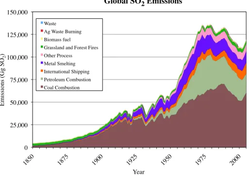
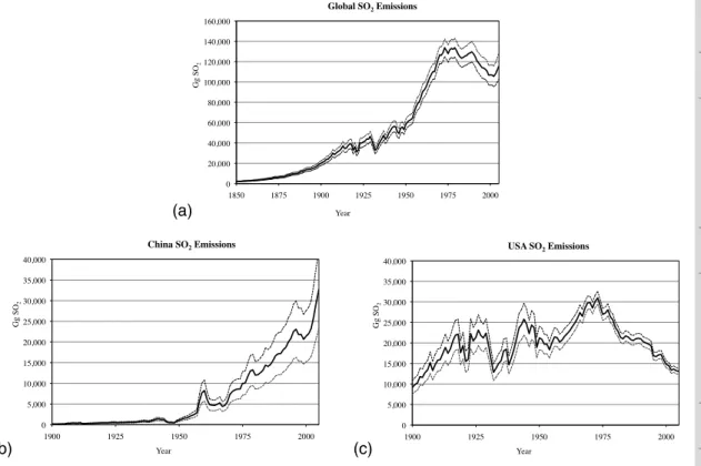
Global SO2emissions from 1850–2005 by sector are shown in Fig. 2. To obtain total
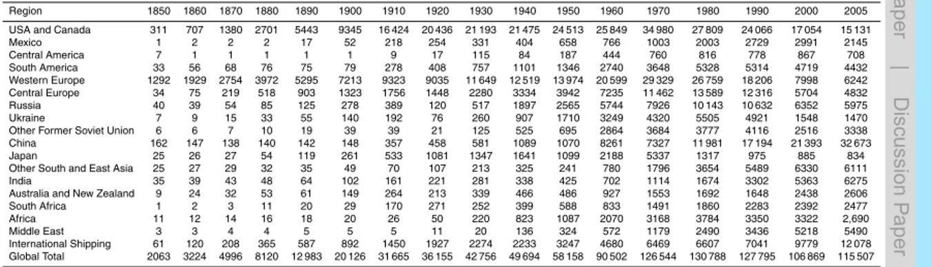
anthropogenic emissions, extrapolated emissions from forest and grassland fires (Van der Werf et al., 2006; Schultz et al., 2008; Mieville et al., 2010) as used in the RCP historical inventory exercise (Lamarque et al., 2010) are also included. Table 1 presents
10
a summary of total emissions, exclusive of open burning, by region for decadal years. Global emissions peaked in the 1970s after a nearly monotonic increase over two decades. Emissions have declined overall since 1990, with an increase between 2002– 2005 due largely to strong growth of emissions in China.
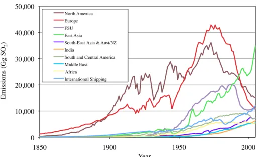
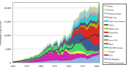
Sectoral and regional emissions trends are shown in Figs. 2 and 3. Emissions from
15
petroleum combustion have become a smaller portion of total emissions, with a large
portion of estimated petroleum SO2emissions now originating from international
ship-ping, a sector where high sulfur bunker fuel could, until recently, be used without restric-tion in most of the world. Trends in emissions from coal combusrestric-tion include a steady decline since the 1970s in Europe and North America combined with large changes
20
in coal combustion in the states of the Former Soviet Union after 1990, and a large increase in coal combustion in China in recent years. Emissions from metal smelting have decreased since their peak around 1970 due to increased sulfur removal, in part due to the widespread introduction of flash smelter technologies.
As seen in previous work (Smith et al., 2001, 2004), we find that there has also been
25
ACPD
10, 16111–16151, 2010Anthropogenic sulfur dioxide emissions:
1850–2005
S. J. Smith et al.
Title Page
Abstract Introduction
Conclusions References
Tables Figures
◭ ◮
◭ ◮
Back Close
Full Screen / Esc
Printer-friendly Version Interactive Discussion
Discussion
P
a
per
|
Dis
cussion
P
a
per
|
Discussion
P
a
per
|
Discussio
n
P
a
per
|
by Europe and North America. Since that time, emissions from other regions, Asia in particular, have increased. Since the mid-1970’s, an increasing fraction of global emissions have originated from Asia. Emissions from other regions (Africa, Middle-East, South America and Latin America) have also increased, but to a lesser extent. Emissions from China have increased to 28% of the estimated global total in 2005.
5
The annual global emissions estimate is similar before 1970 to the previous estimate using similar methodologies (Smith et al., 2001), albeit with some larger regional dif-ferences. Past 1970, the current estimate is lower, due in large part to lower emissions estimates for China and the Former Soviet Union, although emissions in these regions are particularly uncertain.
10
4 Uncertainty
It is useful to examine uncertainty in emissions by source and region. To our knowl-edge, this is the first consistent estimate of global and regional uncertainty in sulfur dioxide emissions. For this estimate, we apply a relatively simple approach to uncer-tainty analysis whereby a set of unceruncer-tainty bounds are applied to broad classes of
15
countries. This is warranted in large part since, as noted by Sch ¨opp et al. (2005), lim-ited data are available to specify parameter uncertainty bounds, leading to bounds that are generally specified through expert judgment. This is particularly true for develop-ing countries. In addition, sulfur dioxide emissions are principally determined by fuel sulfur content and not technology-specific emissions factors, at least in the absence
20
of emissions controls. Data on fuel sulfur content are sparse in general, and those that contain uncertainty information even rarer. These considerations make a more complex assessment of global uncertainty unwarranted at this time.
The first component of the uncertainty analysis considers errors in the individual components of the emissions calculation. The set of uncertainty bounds given in
Ta-25
Uncertain-ACPD
10, 16111–16151, 2010Anthropogenic sulfur dioxide emissions:
1850–2005
S. J. Smith et al.
Title Page
Abstract Introduction
Conclusions References
Tables Figures
◭ ◮
◭ ◮
Back Close
Full Screen / Esc
Printer-friendly Version Interactive Discussion
Discussion
P
a
per
|
Dis
cussion
P
a
per
|
Discussion
P
a
per
|
Discussio
n
P
a
per
|
ties are applied separately in each country to emissions from the following sources: coal, petroleum, biomass, fuel processing, smelting, and other process. Uncertain-ties in each of these categories are assumed to be independent and are combined in quadrature. Conceptually, aggregate uncertainty can be divided into uncertainty in driving forces, such as fuel consumption or smelter metal output, and uncertainty in
5
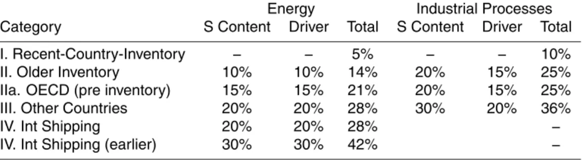
sulfur content (and assumptions such as ash retention) that as shown in Table 2. How-ever, only the total values are used in this calculation. The values in Table 2 are based on the author’s judgment and are similar to other estimates in the literature (Sch ¨opp et al., 2005; Gregg et al., 2008; Eyring et al., 2009).
Because common assumptions and data sources are used for large portions of the
10
world, we assume for simplicity that uncertainties with each sector are perfectly cor-related within 14 world regions. An alternative calculation assuming no correlation between values at the country level results in lower uncertainty at a global level by 3–27%, depending on the year.
This procedure assumes uncertainties are symmetric. This is likely not strictly true
15
since, for example, sulfur removal (for petroleum and metal smelting) is bounded above, sulfur retained in ash is bounded below, and some emissions drivers have potential biases in one direction – for example, underreporting of consumption (Logan, 2001). It is not clear, however, if a more nuanced calculation is warranted given the number of assumptions that would need to be made.
20
The uncertainty estimate calculated as described above results in uncertainty
bounds on annual global total SO2 emissions that are relatively small: 4–8% over the
20th century. This low value is due to cancellation between sectors and regions. This uncertainty level would appear to be unrealistically low given that a number of previous global sulfur dioxide emissions estimates do not fall within this estimated uncertainty
25
bound (Smith et al., 2001; ¨Om et al., 1996; Van Aardenne et al., 2001; Lefohn et al.,
re-ACPD
10, 16111–16151, 2010Anthropogenic sulfur dioxide emissions:
1850–2005
S. J. Smith et al.
Title Page
Abstract Introduction
Conclusions References
Tables Figures
◭ ◮
◭ ◮
Back Close
Full Screen / Esc
Printer-friendly Version Interactive Discussion
Discussion
P
a
per
|
Dis
cussion
P
a
per
|
Discussion
P
a
per
|
Discussio
n
P
a
per
|
moval, and other driver data, methodological assumptions, and the use of common default assumptions for sectors where little data exists. Comparing the present
inven-tory with that of Smith et al. (2004), for example, indicates that the differences between
these two estimates involve several methodological and data changes that impacted emissions estimates over multiple world regions.
5
To include the potential impact of such correlated effects, we add to the uncertainty
estimate for each sector an additional uncertainty amounting to 5% of total emissions (half this value for countries with well-specified inventories), with the additional uncer-tainty combined again in quadrature between sectors. This latter assumption is made since there is little overlap in assumptions between either sulfur contents, emissions
10
controls, or driver data between the broad sectors used in this calculation. The global value of the correlated uncertainty component is less than 3% since 1960, due to a can-cellation across sectors, increasing to 4% by 1920 as emissions from coal combustion become more dominant.
The addition of this correlated component to uncertainty has a large impact on the
15
final uncertainty value. The uncertainty range is increased by a factor of 1.4 to 1.7, depending on the year. Even with this component, however, the global uncertainty in sulfur dioxide emissions over the 20th century is still only 6–12%. The global emis-sions estimate of Smith et al. (2004) now largely falls within this expanded uncertainty range. While this component has a large relative impact on the global uncertainty, the
20
impact of this assumption on regional uncertainties is somewhat smaller. For exam-ple, the largest uncertainty in recent years is in emissions from China. The addition of this correlated component increases the magnitude of the total estimated uncertainty for China emissions by a factor of 1.2 (from 24% of total emissions to 28% of total emissions).
25
ACPD
10, 16111–16151, 2010Anthropogenic sulfur dioxide emissions:
1850–2005
S. J. Smith et al.
Title Page
Abstract Introduction
Conclusions References
Tables Figures
◭ ◮
◭ ◮
Back Close
Full Screen / Esc
Printer-friendly Version Interactive Discussion
Discussion
P
a
per
|
Dis
cussion
P
a
per
|
Discussion
P
a
per
|
Discussio
n
P
a
per
|
the estimated uncertainty in global emissions is±9 000 Gg SO2.
The estimated uncertainty bounds for the United States are also shown in Fig. 4. The uncertainty range for the United States is smaller, even in earlier years, than the
estimate for China. A portion of this difference is due to the assumed lower uncertainty
bounds (Table 2). Also contributing to a lower overall uncertainty estimate is that
emis-5
sions from the United States throughout the 20th century are from a wider variety of sources as compared to China, where emissions are dominated by coal consumption in all periods. This results in a larger statistical cancelation of uncertainties between
sectors in the United States. Offsetting this somewhat is a similar relative impact of
systematic uncertainties.
10
The regional uncertainty values, before combination to global values as described above, are shown in Fig. 5. China is the largest single contributor to emissions
uncer-tainty since about 1980, with an estimated unceruncer-tainty in 2000 of±5200 Gg SO2. The
second largest source of uncertainty in 2005 is emissions from international shipping. The largest contributors to uncertainty have changed over the years, with countries of
15
the Former Soviet Union and Western Europe dominant during the 1960s and 1970s, and the United States dominant during the early to mid-20th century.
Sulfur emissions are less uncertain than emissions of most other air pollutants be-cause emissions depend largely on sulfur contents rather than combustion conditions. There is a large contrast with emissions of another important aerosol, black carbon.
20
Bond et al. (2004) estimated global fossil black carbon emissions in 1996 as 3.0 Tg C,
with an uncertainty range of 2.0–7.4 Tg C, or+150% and−30%, with the upper range
an order of magnitude larger than the uncertainty in sulfur dioxide emissions estimated here.
Note that uncertainty in the spatial allocation was not assessed, but will likely be
25
ACPD
10, 16111–16151, 2010Anthropogenic sulfur dioxide emissions:
1850–2005
S. J. Smith et al.
Title Page
Abstract Introduction
Conclusions References
Tables Figures
◭ ◮
◭ ◮
Back Close
Full Screen / Esc
Printer-friendly Version Interactive Discussion
Discussion
P
a
per
|
Dis
cussion
P
a
per
|
Discussion
P
a
per
|
Discussio
n
P
a
per
|
5 Discussion
In 1850, global sulfur dioxide emissions over land areas were split roughly evenly be-tween emissions from open burning and anthropogenic industrial activities. Over the next 50 years this changed dramatically as anthropogenic sulfur dioxide emissions in-creased by an order of magnitude, driven by inin-creased use of coal. In the early 20th
5
century the steady growth of emissions was slowed by a global depression and the second world war followed by the post war economic expansion, resulting in an
un-precedented absolute rate of emissions growth averaging 3400 Gg/decade from 1950
to 1970.
For most of this period, sulfur dioxide emissions increased in proportion to activity
10
levels. This began to change dramatically after 1970 due to concern over the impacts of these emissions on regional scales. Precursors to this change are evident in smelting and petroleum refining sectors. The amount of sulfur removed from crude oil has been steadily increasing since 1958 (Fig. 1) and a similar pattern exists for metal smelting, where around half the sulfur contained in metal ores was removed at the smelter by
15
1980. Removal of sulfur from coal combustion by means of post-combustion scrubbers began somewhat later, but is now a major driver of sulfur emission reductions. Shifts
in coal supply to favor lower sulfur coal have also been a factor, although it is difficult
to estimate the magnitude of this effect.
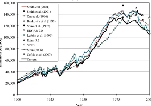
The current estimate is compared to other estimates of global sulfur dioxide
emis-20
sions in Fig. 6. The current estimate is somewhat below many recent estimates, par-ticularly in the 1970s and 1980s, including the previous estimate by Smith et al. (2004)
using a similar methodology, but at a more aggregate scale. The major differences
be-tween these two datasets over this time period are lower emissions estimates for China
and the countries of the Former Soviet Union. Other differences include updated
infor-25
ACPD
10, 16111–16151, 2010Anthropogenic sulfur dioxide emissions:
1850–2005
S. J. Smith et al.
Title Page
Abstract Introduction
Conclusions References
Tables Figures
◭ ◮
◭ ◮
Back Close
Full Screen / Esc
Printer-friendly Version Interactive Discussion
Discussion
P
a
per
|
Dis
cussion
P
a
per
|
Discussion
P
a
per
|
Discussio
n
P
a
per
|
country inventory data for many OECD countries.
The uncertainty bounds estimated in Sect. 4 encompass many of the other esti-mates, although the Spiro et al. (1992) and EDGAR 3.2 (Olivier and Berdowski, 2001) estimates lie above the uncertainty range, as does the estimated year 2000 emissions data point used in the SRES emissions scenarios. The uncertainty analysis conducted
5
here highlights the potential importance of systematic errors and biases in emissions estimates, particularly for emissions such as sulfur dioxide, where most input values are only weakly correlated between regions. While the uncertainty estimates here are based on the authors’ judgment, the relatively small global uncertainty that results indi-cates that a more complex global uncertainty analysis may not be warranted. Regional
10
uncertainty can be far higher than global uncertainty, however, and more detailed un-certainty analysis of high-emitting regions may be useful to better bound current and past environmental impacts of sulfur dioxide emissions.
When comparing data sets, it should be noted that most of these estimates rely on similar, if not identical, data sets for historical fossil fuel use and for historical emissions
15
from Europe and the United States. Errors or biases in these data, such as the
ap-parent underestimate of SO2 emissions from petroleum products in the United States
prior to 1980, are likely to be common to most of these estimates. As demonstrated in Sect. 4, methodological biases and systematic errors can make a large contribution
to uncertainty, particularly for SO2emissions, which depend on characteristics that are
20
largely uncorrelated between regions.
It is also useful to compare 2005 emissions with previous estimates from global
sce-nario projections. The 2005 emissions, estimated here as 115 510±12 850 Gg, largely
overlap with the range of future SO2 emissions scenarios from Smith et al. (2005).
This range is significantly lower than the SRES scenario projections for 2005, but does
25
ACPD
10, 16111–16151, 2010Anthropogenic sulfur dioxide emissions:
1850–2005
S. J. Smith et al.
Title Page
Abstract Introduction
Conclusions References
Tables Figures
◭ ◮
◭ ◮
Back Close
Full Screen / Esc
Printer-friendly Version Interactive Discussion
Discussion
P
a
per
|
Dis
cussion
P
a
per
|
Discussion
P
a
per
|
Discussio
n
P
a
per
|
Emissions in Asia are of particular interest and it is useful to compare emissions here with previous estimates. As shown in the supplementary material, even recent
estimates for SO2 emissions in Asia (Ohara et al., 2007; Streets et al., 2003; Zhang
et al., 2009; Klimont et al., 2009) sometimes differ substantially. Focusing on China
and India, the two countries with the largest emissions, these recent estimates all lie
5
within the uncertainty range estimated here, with the REAS estimate for 2000 consis-tently larger than the other estimates quoted here, but near the upper bound of our uncertainty range for both China and India (although 1% over our uncertainty bound for India). The estimate here for China is within a few percent of the estimate in Lu et al. (2010) for 2000–2005. The current estimate for India is close to the estimate from
10
Garg et al. (2006) in 1985 but diverges to be 30% higher than the Garg et al. value by 2005, but similar to other recent inventories (supplementary material).
The current estimate for China is 20–30% lower than earlier estimates based on
the RAINS Asia project (Arndt et al., 1997; Streets et al., 2000; Streets and Waldhoff,
2000; Klimont et al., 2001) for 1895–1990. This difference is within the estimated
15
uncertainty range. While the current estimate for India for 2000 and 2005 is similar to a number of other regional estimates for these years (although higher than Garg et al., 2006), the current estimate is 40% lower than the circa 1987 estimates from Arndt et al.
(1997) and Streets et al. (2000). Note that such historical differences are not limited to
developing countries, as indicated above (Sect. 2.1) for past emissions from petroleum
20
in the United States.
It is not clear if such historical differences are due to variation in energy
consump-tion data, parameter assumpconsump-tions such as sulfur content or ash retenconsump-tion fracconsump-tion, or
other methodological differences, such as treatment of shifts in petroleum product
con-sumption and sulfur contents. Analysis of these differences is beyond the scope of the
25
ACPD
10, 16111–16151, 2010Anthropogenic sulfur dioxide emissions:
1850–2005
S. J. Smith et al.
Title Page
Abstract Introduction
Conclusions References
Tables Figures
◭ ◮
◭ ◮
Back Close
Full Screen / Esc
Printer-friendly Version Interactive Discussion
Discussion
P
a
per
|
Dis
cussion
P
a
per
|
Discussion
P
a
per
|
Discussio
n
P
a
per
|
emission parameters will translate directly into uncertainty in total emissions. A his-torical analysis of coal production and consumption in China, particularly data on coal production by source in order to track changing sulfur contents, would be especially useful in better determining historical emissions.
Future estimates of historical sulfur dioxide emissions could be improved through
5
improved regional data sets for fossil fuel consumption, fuel properties, and industrial process drivers (including metal smelting amounts, ore properties, sulfuric acid pro-duction, and pulp and paper production). Limited information was available for sulfur dioxide emissions resulting from petroleum and natural gas extraction operations and the use of sour gas, even though these sources could be regionally significant. Many
10
historical data series are only readily available at the country level. Improved spatial estimates of historical emissions would require sub-national consumption and activity information, particularly for geographically large countries such as the United States, Russia, and China.
Differences among estimates of both current and past emissions point to the need
15
for further research to identify current and historical fuel sulfur contents and the char-acteristics of fuel-emissions technology combinations (such as sulfur retention in ash). While the bottom-up estimation methods used, in part, in this work are appropriate for countries with few emissions controls, direct emissions monitoring of large sources will become even more important for accurate emission estimates as the use of sulfur
20
control technologies becomes more widespread.
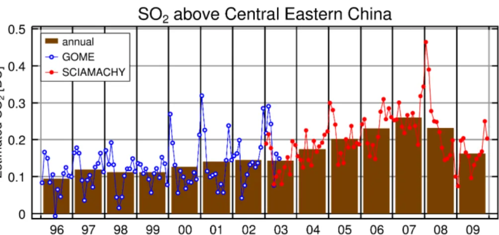
The use of satellite observations (Krotkov et al., 2008; Li et al., 2010; Lu et al., 2010; Gottwald et al., 2010) to verify trends shows promise, although estimation of
absolute emission values through use of satellite data is more difficult. Figure 7 shows
the SO2 column concentration above Eastern China as estimated by Gottwald et al.
25
(2010) using satellite data. The increase in estimated SO2 column from 2000 to 2005
is about 1.5, which is the same change as in total emissions over China from this
pe-riod. The comparison for the earlier period is less clear. The change from 1996/1997
ACPD
10, 16111–16151, 2010Anthropogenic sulfur dioxide emissions:
1850–2005
S. J. Smith et al.
Title Page
Abstract Introduction
Conclusions References
Tables Figures
◭ ◮
◭ ◮
Back Close
Full Screen / Esc
Printer-friendly Version Interactive Discussion
Discussion
P
a
per
|
Dis
cussion
P
a
per
|
Discussion
P
a
per
|
Discussio
n
P
a
per
|
the inventory estimate decreases over this period, taking the average over the indicated
years. Part of this difference could be due to shifts in SO2source distribution over this
time period. Concentrated emissions from large sources, which are also lofted higher into the atmosphere, are more likely to be detected by satellite instruments. From 1995 to 2000, we estimate that fraction of total emissions from power plants in China
5
increased from 46% to 60%, which is in the right direction to help explain the diff
er-ence in trends. Meteorological and atmospheric chemistry effects on SO2 transport
and lifetime will also affect the relationship between SO2 column measurements and
emissions. Additional uncertainty arises from changes in aerosol loading leading to changes in satellite sensitivity. See Gottwald et al. (2010) and the papers cited above
10
for further discussion of these effects. It is not yet clear how these uncertainties on the
detection side compare to the uncertainty in the inventory-based emissions estimate as quantified here.
Historical estimates of sulfur dioxide emissions are necessary for estimating past trends in acid deposition, the associated impacts, and past climate forcing. The current
15
estimate represents a consistent global data set with annual resolution that can be used for historical modeling studies. The annual emissions data described in this paper are
available from the corresponding author. The 0.5◦ gridded emissions data released
for the RCP project are available at the RCP web site (see also the supplementary material).3
20
Supplementary material related to this article is available online at: http://www.atmos-chem-phys-discuss.net/10/16111/2010/
acpd-10-16111-2010-supplement.pdf.
Acknowledgement. Work at PNNL on this project was supported by the Department of Energy
Office of Science. Z. Klimont and GAINS work was supported by ACCENT and EUCAARI. The
25
authors would like to thank E. Chapman for a very useful internal review, A. Richter for Fig. 7
3
ACPD
10, 16111–16151, 2010Anthropogenic sulfur dioxide emissions:
1850–2005
S. J. Smith et al.
Title Page
Abstract Introduction
Conclusions References
Tables Figures
◭ ◮
◭ ◮
Back Close
Full Screen / Esc
Printer-friendly Version Interactive Discussion
Discussion
P
a
per
|
Dis
cussion
P
a
per
|
Discussion
P
a
per
|
Discussio
n
P
a
per
|
and helpful comments, and the many colleagues and organizations that shared data used in this project. We also thank M. Nathan and T. Weber for assistance with formatting.
References
Andreae, M. O. and Merlet, P.: Emissions of trace gases and aerosols from biomass burning, Global Biogeochem. Cy., 15, 955–966, doi:10.1029/2000GB001382, 2001.
5
Andres, R. J., Fielding, D. J., Marland, G., Boden, T. A., and Kumar, N.: Carbon dioxide emis-sions from fossil-fuel use, 1751–1950, Tellus, 51, 759–765, 1999.
Arndt, R. L., Carmichael, G. R., Streets, D. G., and Bhatti, N.: Sulfur dioxide emissions and sectorial contributions to sulfur deposition in Asia, Atmos. Environ., 31, 1553–2310, doi:10.1016/S1352-2310(96)00236-1, 1997.
10
Benkovitz, C. M., Scholtz, M. T., Pacyna, J., Tarras ´on, L., Dignon, J., Voldner, E. C., Spiro, P. A., Logan, J. A., and Graedel, T. E.: Global gridded inventories of anthropogenic emissions of sulphur and nitrogen, J. Geophys. Res, 101(D22), 29239–29253, doi:10.1029/96JD00126, 1996.
Bingham, T. H., Cooley, P. C., Fogel, M. E., Johnston, D. R., LeSourd, D. A., Miedema, A. K., 15
Paddock, R. E., Simons Jr., M., and Wisler, M. M.: A projection of the effectiveness and
costs of a national tax on sulfur emissions final report, Research Triangle Institute, Research Triangle Park, North Carolina, RTI Project No. 41U-757, 1976.
Bond, T. C., Bhardwaj, E., Dong, R., Jogani, R., Jung, S., Roden, C., Streets, D. G., and Trautmann, N. M.: Historical emissions of black and organic carbon aerosol from energy-20
related combustion, Global Biogeochem. Cy., 21, GB2018, doi:10.1029/2006GB002840, 1850–2000, 2001.
Bond, T. C., Streets, D. G., Yarber, K. F., Nelson, S. M., Woo, J.-H., and Klimont, Z.: A technology-based global inventory of black and organic carbon emissions from combus-tion, J. Geophys. Res., 109, D14203, doi:10.1029/2003JD003697, 2004.
25
Center for International Earth Science Information Network (CIESIN), Columbia University; and Centro Internacional de Agricultura Tropical (CIAT), Gridded Population of the World Version 3 (GPWv3): Population Density Grids, Palisades, NY, Socioeconomic Data and Applications Center (SEDAC), Columbia University, available at: http://sedac.ciesin.columbia.edu/gpw, 2005.
ACPD
10, 16111–16151, 2010Anthropogenic sulfur dioxide emissions:
1850–2005
S. J. Smith et al.
Title Page
Abstract Introduction
Conclusions References
Tables Figures
◭ ◮
◭ ◮
Back Close
Full Screen / Esc
Printer-friendly Version Interactive Discussion
Discussion
P
a
per
|
Dis
cussion
P
a
per
|
Discussion
P
a
per
|
Discussio
n
P
a
per
|
Cofala, J., Amann, M., Klimont, Z., Kupiainen, K., and H ¨oglund-Isaksson, L.: Scenarios of global anthropogenic emissions of air pollutants and methane until 2030, Atmos. Environ., 41(38), 8486–8499, doi:10.1016/j.atmosenv.2007.07.010, 2007.
Eggleston, S., Buendia, L., Miwa, K., Ngara, T., and Tanabe, K. (Eds.): 2006 IPCC Guide-lines for National Greenhouse Gas Inventories, Intergovernmental Panel on Climate Change, 5
IGES, Japan, 2006.
Endresen, Ø., Sørgard, E., Behrens, H. L., Brett, P. O., and Isaksen, I. S. A.: A historical reconstruction of ships’ fuel consumption and emissions, J. Geophys. Res., 112, D12301, doi:10.1029/2006JD007630, 2007.
Energy Information Administration (EIA 2008): International Energy Annual 2006, Washington 10
DC, http://www.eia.doe.gov, 2004.
Energy Information Administration (EIA 2009), Annual Energy Review 2008, Washington DC, DOE/EIA-0384, 2009.
Environment Canada: 1985–2006 Historical SOx Emissions for Canada (Version 2, 8 April
2008), http://www.ec.gc.ca/, 2008. 15
Etemad, B., Bairoch, P., Luciani, J., and Toutain, J.-C.: World energy production 1800–1985, Libraire Droz, Geneve, 272 pp., 1991.
European Environment Agency (EEA): Anthropogenic emissions of sulphur (1980–2010) in the ECE region (September 2000), 2002.
Eyring, V., Isaksen, I. S. A., Berntsen, T., Collins, W. J., Corbett, J. J., Endresen, O., 20
Grainger, R. G., Moldanova, J., Schlager, H., and Stevenson, D. S.: Transport impacts on atmosphere and climate: shipping, Atmos. Environ., doi:10.1016/j.atmosenv.2009.04.059, in press, 2009.
FAOSTAT: http://faostat.fao.org/, accessed: March 2009.
Fernandes, S. D., Trautmann, N. M., Streets, D. G., Roden, C. A., and Bond, T. C.: Global biofuel 25
use, 1850–2000, Global Biogeochem. Cy., 21, GB2019, doi:10.1029/2006GB002836, 2007. Fletcher, M. E.: From coal to oil in British shipping, in: The World of Shipping, edited by:
Williams, D. M., Aldershot, Hants, England, Ashgate, Brookfield VT, 1997.
Foell, W., Amann, M., Carmichael, G., Chadwick, M., Hettelingh, J., Hordijk, L., and Dianwu, Z. (Eds.): RAINS-Asia: an assessment model for air pollution in Asia, 1995.
30