www.ann-geophys.net/29/251/2011/ doi:10.5194/angeo-29-251-2011
© Author(s) 2011. CC Attribution 3.0 License.
Annales
Geophysicae
Secular trends in storm-level geomagnetic activity
J. J. Love
Geomagnetism Program, US Geological Survey, Denver, CO, USA
Received: 20 December 2010 – Accepted: 19 January 2011 – Published: 3 February 2011
Abstract. Analysis is made of K-index data from groups of ground-based geomagnetic observatories in Germany, Britain, and Australia, 1868.0–2009.0, solar cycles 11–23. Methods include nonparametric measures of trends and sta-tistical significance used by the hydrological and climato-logical research communities. Among the three observatory groups, GermanKdata systematically record the highest dis-turbance levels, followed by the British and, then, the Aus-tralian data. Signals consistently seen inK data from all three observatory groups can be reasonably interpreted as physically meaninginful: (1) geomagnetic activity has gen-erally increased over the past 141 years. However, the de-tailed secular evolution of geomagnetic activity is not well characterized by either a linear trend nor, even, a monotonic trend. Therefore, simple, phenomenological extrapolations of past trends in solar and geomagnetic activity levels are unlikely to be useful for making quantitative predictions of future trends lasting longer than a solar cycle or so. (2) The well-known tendency for magnetic storms to occur during the declining phase of a sunspot-solar cycles is clearly seen for cycles 14–23; it is not, however, clearly seen for cycles 11–13. Therefore, in addition to an increase in geomagnetic activity, the nature of solar-terrestrial interaction has also ap-parently changed over the past 141 years.
Keywords. Magnetospheric physics (Solar wind-magnetosphere interactions)
1 Introduction
In considering the possibility of trends in data time series, careful consideration should be given to: (1) the meaning of the word “trend”. It is context-dependent. It might be de-fined as a general direction or tendency, or as the longest, non-periodic movement of a time series (e.g. Dagum and
Correspondence to:J. J. Love (jlove@usgs.gov)
Dagum, 1988). And while many people might claim to rec-ognize a trend when they see one, a more precise, but still usefully general, definition is difficult to pronounce (e.g. Preece, 1987). We are reminded of the limerick by Cairn-cross (1969): “A trend is a trend is a trend . . . ”. To which we would unpoetically add the hope that a graph of the data would have a visually-compelling slope. Of course, needed specificity for what is meant by “trend” can be obtained through (2) measuring and testing. These typically involve either deterministic or stochastic analysis, with limitations imposed by data quantity and quality, and the possible pres-ence of superimposed signals. Here, the notion of signifi-cance is important, as is the timescale over which the trend is supposed to apply. And there are practical considerations, why we might be interested in a trend: its (3) utility. An es-timated trend can serve as a summary property of available data. But for many applications, prediction is the goal, or to paraphrase Cairncross: does the trend bend, and come to an end? The combination of describing data collected in the past, predicting future data or, at least, predicting those that have yet to be seen, and, then, making objective comparisons is the basis of hypothesis testing. This formal approach is of-ten conducted in laboratory settings, where experiments can be actively controlled, but it is not always so straightforward for many of the “natural” sciences, where we only observe the phenomena provided by Nature.
252 J. J. Love: Secular trends in storm-level geomagnetic activity
Table 1.Summary of the observatories for whichKindices are used.
Group Observatory Country Code Geomag. lat. CGM lat. Data years Present institute Potsdam Germany POT 52.11◦ 48.32◦ 1890.0–1908.0
PSN Seddin Germany SED 52.02◦ 48.21◦ 1908.0–1932.0
Niemegk Germany NGK 51.88◦ 47.97◦ 1932.0–2009.0 GeoForschungsZentrum
Greenwich Great Britain GRW 53.57◦ 47.75◦ 1868.0–1926.0
GAH Abinger Great Britain ABN 53.35◦ 47.42◦ 1926.0–1957.0
Hartland Great Britain HAD 53.90◦ 47.48◦ 1957.0–2009.0 British Geological Survey
Melbourne Australia MEL −45.74◦
−48.68◦ 1868.0–1920.0
MTC Toolangi Australia TOO −45.38◦ −48.30◦ 1920.0–1980.0
Canberra Australia CNB −42.71◦ −45.39◦ 1980.0–2009.0 Geoscience Australia
one in Britain and one in Australia. The aa index is the longest-running, standard, geomagnetic-activity time se-ries available. It records several signals, including solar-cycle modulation of geomagnetic activity and an apparent long-term trend of increasing geomagnetic activity. Both of these signals are of numerous and far-reaching conse-quence for (1) magnetic-storm occurrence statistics and time-series analysis (Delouis and Mayaud, 1975; Clilverd et al., 1998; Echer et al., 2004), (2) space-weather hazards (Oler, 2004; Welling, 2010), (3) solar-terrestrial interaction (Schat-ten and Wilcox, 1967; Feynman and Crooker, 1978; Lock-wood et al., 1999), (4) solar activity and space-weather pre-diction (Feynman and Gu, 1986; Rangarajan and Barreto, 1999; Hathaway, 2010), (5) terrestrial climate change (Bucha and Bucha, 1998; Friis-Christensen, 2000; Courtillot et al., 2007), (6) atmospheric ozone depletion (Laˇstoviˇcka et al., 1992), and (7) cosmic rays and atmospheric radionuclide production (Stuiver and Quay, 1980; McCracken, 2004).
But the fidelity of the aa time series has been the sub-ject of a debate played out in the scientific literature. Its sourceK-index values can be artificially affected in a num-ber of ways. (1) Localized magnetotelluric signals, which are different from site to site, would factor in observatory relocations (Mayaud, 1973). (2) Changes in observatory in-strumentation and accuracy from one analog system to an-other (Clilverd et al., 2002) and from analog systems to dig-ital systems. (3) Normalization factors needed to accommo-date different observatory magnetic latitudes (Clilverd et al., 1998). (4) Changes of convention in the magnetic-vector components used to estimateK values. (5) Changes inK -estimation methods, especially from hand-scaling of analog magnetograms to computer-algorithm estimation using dig-ital data. While various authors (e.g. Clilverd et al., 2005; Lukianova et al., 2009) have concluded that none of these factors significantly affect the long-term trend of increasing geomagnetic activity seen in theaa time series, Svalgaard et al. (2004) assert that theaaindex needs substantial recal-ibration, and that if this were properly done, any trend of in-creasing activity would be substantially reduced, possibly so
much that it would be of little or no long-term significance. If this were true, then it might also affect interpretations of the relationship between solar activity and geomagnetic ac-tivity, since it is clear that sunspot number has exhibited sec-ular change since the middle of the 19th century. Linger-ing concerns have motivated the introduction of several new global, geomagnetic-activity indices (Mursula and Martini, 2007; Svalgaard and Cliver, 2007; Finch et al., 2008).
With a goal of obtaining an improved understanding of how to measure and how to interpret secular change in geo-magnetic activity, here, we focus our attention on the source Kindices from Britain and Australia that have been used to calculateaa values, and, for comparison, we also examine K indices from Germany that, in some respects, are the in-ternational standard. In contrast to the methods used to cal-culateaa, and, indeed, in contrast to many of the methods used to analyzeaa, we do not adjust theK values in any way. We analyze theK-value data as they were originally reported using standard statistical and time series methods, some of which are used for trend estimation in the hydrology and climatology research communities. Comparison ofK values from different observatory groups reveals some sig-nificant and, in some respects, unfortunate inconsistencies and biases. They also reveal some prominent and important consistencies and patterns. The latter can help us confidently answer the question of whether or not geomagnetic activity exhibits a long-term increasing trend and, also, change in its phase relationship with sunspot number.
2 Data
2.1 K-index values
Table 2.Summary of magnetic-activity ranges associated with eachK-index value for each observatory.
K 0 1 2 3 4 5 6 7 8 9
PSN, GAH, MEL, TOO 0–5 5–10 10–20 20–40 40–70 70–120 120–200 200–330 330–500 500–∞ (nT) CNB 0–4.5 4.5–9 9–18 18–36 36–63 63–108 108–180 180–297 297–450 450–∞ (nT)
of the range of irregular geomagnetic fluctuations recorded at a magnetic observatory, after solar and lunar quiet-time daily variation and slow variation associated with magnetic-storm recovery have been subtracted (Bartels et al., 1939, p. 412).Kvalues are “ordinal”: they are ranked, dimension-less integers, ranging from 0 for the quietest magnetic condi-tions, through to 5 for what are usually considered to be mild magnetic-storm levels (www.swpc.noaa.gov/NOAAscales), up to 9 for the most disturbed conditions, all according to a scale that is approximately the logarithm of the absolute range of magnetic-field variation measured over 3-h inter-vals of time at Niemegk. After its introduction, theKindex was calculated retrospectively from historical analog mag-netograms from several observatories, extending theKtime series backwards in time to the 19th century.
To facilitate inter-comparison of magnetic-field variation from observatories at different locations, especially across a range of latitudes, the long-term statistical distributions ofK values collected at a particular observatory are supposed to be normalized so that they are like that realized at Niemegk (Bartels et al., 1940, pp. 334-335). But this is not what has actually been done. Instead, K values are derived from a scale developed by Mayaud (1968): a lower-limit forK=9 is assigned according to a phenomenologically-derived for-mula relating an observatory’s corrected-geomagnetic lati-tude (CGM) to an expected probability for a high-activity range of magnetic-field variation as measured in nT, see Ta-ble 2. Since this scaling is not, itself, derived from any physics-based theory, it is an arbitrary quantization, and, as a result, K-index distributions from different observatories will, inevitably, be different from each other.
In this study, we useK indices from the nine magnetic observatories listed in Table 1: three groups of three ob-servatories from Germany PSN, Great Britain GAH, and Australia MTC that are situated at approximately the same corrected-geomagnetic latitudes. The observatories in each group have operated in series; with the closure of one ob-servatory another one was opened at a nearby site in or-der to maintain continuity. Together, these K-index time series are among the longest available for studies of secu-lar change in geomagnetic activity. We obtained the Ger-manK values, 1890.0–2009.0, from H.-J. Linthe (personal communication, 2010), GeoForschungsZentrum, the British K values, 1868.0–2009.0, from the British Geological Sur-vey website (www.geomag.bgs.ac.uk), the Australian CNB K values, 1980.0–2009.0, from the Geoscience Australia website (www.ga.gov.au/geomag/), and the Australian MEL
and TOO values, 1868.0-1980.0, values from P. G. Crosth-waite (personal communication, 2010), Geoscience Aus-tralia, who, in turn, obtained them from M. Menvielle. 2.2 Sunspot numbers
For comparison of geomagnetic-storm occurrence with solar activity, we use sunspot numbersG: for 1868.0–1995.0, so-lar cycles 11–22, we use group numbers (Hoyt and Schatten, 1998) obtained from NOAA’s National Geophysical Data Center (NGDC) website (www.ngdc.noaa.gov), for 1996.0– 2009.0, solar cycle 23, we use international numbersZ ob-tained from the website of the Royal Observatory, Belgium (www.sidc.be). We note thatGis more simply defined than Z, thatGis based on more source observations thanZ, and that G is generally considered to be an improvement over Z (e.g. Hathaway et al., 2002; Kane, 2002). For 1890.0– 1995.0, solar cycles 13–22,GandZare very consistent, but earlier on there are some significant discrepancies (see Hoyt and Schatten, 1998, Fig. 8). This is due, in part, to Wolf’s (1875) practice of adjusting his estimates of sunspot num-ber according to an expectation that they would be correlated in time with ground magnetometer data, which were abail-able to Wolf and his colleagues (Hoyt and Schatten, 1998, p. 497). While this might be considered acceptable for some types of research work (e.g. Svalgaard, 2007), such as repair of defective data or filling in gaps, for our work, where we choose to examine and test the correlation between sunspot number and geomagnetic activity, Wolf’s adjustments are not acceptable. Correlations between data sets that have not in-dependently acquired are not particularly meaningful (see, also, Mursula et al., 2009). For all of these reasons we prefer to useGrather thanZ. In our discussion of results, we define the beginning and the end times of each solar cycle, rounded the the nearest year, according to sunspot-number minimum.
3 Koccurrence time series
254 J. J. Love: Secular trends in storm-level geomagnetic activity
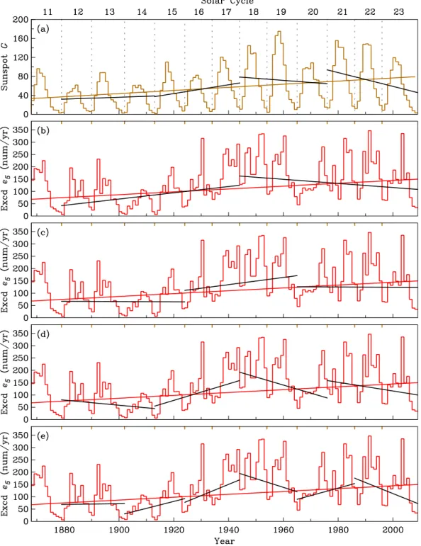
Fig. 1.Time series of(a)annual means of sunspot numbersG, and for German PSN, British GAH, and Australian MTC observatory groups:
(b)annual exceedance count ratese7,(c)annual exceedance count ratese5, and(d)annual attainment count ratesa1. Straight-lines are fitted
to solar-cycle averaged data; example histograms shown in(a), but for clarity omitted from(c)and(d). Compare with Fig. 4.
change in sunspot number and geomagnetic activity that is apparent over the 141-year duration of theGandKtime se-ries. We can quantify this by comparing, for example, the cumulativePje5(tj)of exceedance counts from 2 separate
periods of time, each encompassing 5 solar cycles: for solar cycles 13–17, 1890.0–1944.0, the cumulative exceedances are PSN: 6337, GAH: 4667, and MTC: 3553, while later on, for cycles 19–23, 1954.0–2009.0, they are 8719, 6946, and 5310; increases of 37, 48, and 49%. The cumulative e7 exceedance counts are, of course, smaller than those for
e5 – some years do not have anye7 occurrences – but the
e7 do show a long-term increase; see Fig. 1b. With respect
to low-activity attainment statistics, for solar cycles 13–17,
cumulativea1attainments are PSN: 69 371, GAH: 83 476,
and MTC: 91 392, while later on, for cycles 19–23, they are 45 174, 53 137, and 69 906; decreases of 53, 57, and 30%. From Fig. 1d, we note that many of the maxima of a1 for cycles 19–23 are less than the minima of a1 for
Although each of the three independently-acquired PSN, GAH, and MTCK-value data sets show a long-term, secu-lar increase in geomagnetic activity, systematic differences are also noteworthy. Briefly, the statistical distributions ofK indices are different from one observatory to another. Many factors can contribute to this, some of which are natural and others of which are certainly artificial. In some respects, this is unfortunate, since this is not what Bartels intended when he designed the K index. Still, consistent signals can be seen inKtime series from different observatories, and these can reasonably be interpreted in terms of global, geophysical phenomena.
Focussing on these consistencies, year-to-year cross-correlation is clearly seen between the quantities shown in Fig. 1. This can be quantified in terms of the Pearson correla-tion coefficientrand probabilitypthat the correlation could be realized from random data (Press et al., 1992, “pearsn”). As examples, Pearson coefficients r between observatory pairs of exceedancese5 are PSN-GAH: 0.97, GAH-MTC:
0.95, and MTC-PSN: 0.93, where, in each case,p <10−51.
These observations are not surprising – magnetic disturbance measured byK indices is usually a global phenomenon, so correlation is expected to be “significant”. With respect to cross-correlations between sunspot numbersG ande5, the
Pearson coefficientsrare PSN: 0.44, GAH: 0.47, and MTC: 0.57, where, in each case,p <10−7. Geomagnetic activity
is driven by solar activity, but it is also well-known that peak magnetic activity lags, by a year or two, sunspot maximum. We will explore this relationship in more detail in Sect. 7. For now, we simply emphasize the apparent long-term corre-lation that is seen between three independently-acquiredK time series and sunspot number. This observation can be compared with others based on theaa index (e.g. Legrand and Simon, 1989, Fig. 1; Clilverd et al., 1998, Fig. 2; Ouat-tara et al., 2009, Fig. 2).
4 Linear trends inK
The straightforward observation, taken from Fig. 1, that there is a trend of increasing geomagnetic disturbance over the past 141 years, motivates the testing of straight-line functional fits toK-index counts. Such fits can serve as estimates of “lin-ear trend” (e.g. Woodward and Gray, 1993; Cohn and Lins, 2005), and they have been used in studies of secular change in geomagnetic activity (e.g. Feynman and Crooker, 1978; Lockwood et al., 1999; Mursula and Martini, 2006). To legit-mately accomplish such fits, one must first either remove, as much as is practically possible, serial correlation in the data time series, by, for example, “pre-whitening” or “pruning” the data (e.g. von Storch, 1995, Sect. 2.3), or, alternatively, by using a fitting algorithm that explicitly accommodates serial correlation (e.g. Weatherhead et al., 1998). Year-to-year serial correlation is, of course, especially strong within each solar cycle. We choose to remove it by simply
aver-aging sunspot numbersG, exceedancese5, and attainments
a1within each of theNS solar cycle. For the German PSN
observatories this leaves us with 11 data, one for each solar cycle from 1890.0–2009.0, and for the British GAH and Aus-tralian MTC observatories it leaves us with 13 data covering 1868.0–2009.0. A straight line, “linear trend” is then fitted to the solar-cycle averaged data using an ordinary least-squares algorithm (Press et al., 1992, “fit”), which minimizes the sum of squared residual differences1; fits are shown in Fig. 1.
The fits of linear trends highlight some observations we have already made, namely, that the amount of geomagnetic disturbance has generally increased over the past 141 years. That linear trends can be resolved means that it is neces-sary that a regressive model be time-dependent. Fitted linear trends are not, however, necessarily sufficient descriptions of the data. One way of checking the adequacy of the lin-ear fits is to measure their Plin-earson coefficients r with the data; for the exceedancese5they are PSN: 0.54, GAH: 0.62,
and MTC: 0.64, where, in each case,p <10−1. While these
modest correlations are not likely to be accidental, they do invite scrutiny. From inspection of the residuals in Fig. 1, it is not hard to see that secular variation seen in thee5anda1
could be better fitted by a smooth curve instead of a straight line. With respect to the fitted linear trend for sunspot num-bersG, the Pearson coefficientr is 0.76, wherep <10−2.
Here, as well, a smooth curve might provide a better fit (see, for example, Kishcha et al., 1999, Fig. 11; Svalgaard and Cliver, 2007, Figs. 6 and 7), but solar-terrestrial theory is in-sufficiently developed to provide a specific predictive param-eterization for secular change in sunspot numbers and corre-sponding geomagnetic activity.
The long-term persistence of linear trends can be explicitly checked by fitting subset durations of the available data (see related discussions in Percival and Rothrock, 2005; Kout-soyiannis, 2006). In Fig. 2 we show linear fits to different durations of the British GAH exceedance datae5and an
ex-ample of fits to subset durations of the sunspot data. While fits to data across all 13 solar cycles seem to show a linear trend of increasing geomagnetic disturbance, fits to shorter durations, such as for 6, 4, 3, or 2 cycles, do not consis-tently show persistence. Indeed, Figs. 1 and 2 show that the time-dependence of past geomagnetic activity has been com-plicated. Clearly, our observation of a long-term linear trend of increased geomagnetic disturbance is due, in part, to the time span we have considered, the span of the available ge-omagneticK time series, 13 solar cycles. This is a simple, but important, observation that has been made by others (e.g. Richardson et al., 2002, Fig. 1; Mursula et al., 2004, Fig. 3). If we had chosen to analyze the time span of (say) the past 6 solar cycles, we would, instead, be discussing a decreasing trend in geomagnetic disturbance!
1The linear trends we report here, estimated by an least-squares
256 J. J. Love: Secular trends in storm-level geomagnetic activity
Fig. 2. Comparisons of straight-line fits to sunspot numbersGusing 13 solar cycles of data and(a)3-solar-cycle subset durations of the data. Similarly, comparisons of straight-line fits to exceedancese5from British GAH observatories using 13 solar cycles of data and(b)6,
(c)4,(d)3, and(e)2-solar-cycle subset durations of the data.
The slopes of the linear fits shown in Fig. 1 for the annual exceedances e5 are PSN: 0.69, GAH: 0.58, and
MTC: 0.39 number/yr/century; annual attainments a1 are
PSN:−656.84, GAH:−749.17, and MTC:−503.23 num-ber/yr/century. Thus, the observatory group with the most
rapidly increasing rate of disturbance, as measured by e5,
German PSN, is not the observatory group with the most rapidly decreasing rate of quiescence, as measured by a1,
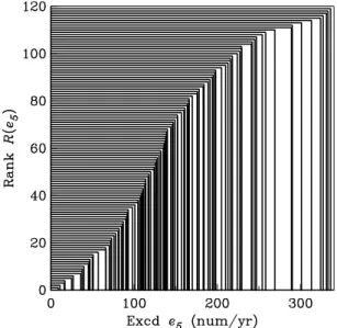
Fig. 3. Schematic representation of the mapping between the or-dered set of German PSNK-exceedance count ratese5and their
ranksRj(e5).
It might also be evidence that secular change in geomagnetic activity is a function of geographic location, as found, for example, by Mursula and Martini (2006, Table 3) in their analyses of observatory, hourly-vector data spanning the 20th century.
5 Ranks ofKover time
Given that the distributions ofKvalues are different for each observatory group, a nonparametric inter-comparison is ap-propriate (e.g. Ferguson, 1965). For this, we rank the data. ForNY exceedancese5, one for each yearj=1,2,3· · ·NY,
the largest has the highest rank and is assigned the number NY, the next largest is assigned the numberNY−1, etc. We represent the operation of assigning ranks to the exceedance data by the mappinge5(tj)→Rj(e5); see Fig. 3. Similar
rankings are be made for the exceedancese7, attainmentsa1,
and sunspot numbersG. By plotting ranks in place of the data themselves, Fig. 4,K-exceedance counts are now neatly normalized, year-to-year correlation is very clear, despite the differentK-occurrence rates at each observatory; compare with the dimensional results shown in Fig. 1.
Data ranking can also be used to confirm the relative in-crease in geomagnetic disturbance that has occurred over the past 141 years. In Table 3 we list the 10 years from 1868.0– 2009.0 with the highest (lowest) levels of geomagnetic activ-ity, as measured by ranks ofe7ande5(a1) from British GAH
and Australian MTC observatories; we also list the 10 years with the highest (lowest) sunspot numbersG. With very few exceptions, which we highlight in Table 3, the most (least) active years measured in terms ofe5(a1) tend to occur in the
second (first) half of the time series, after (before) 1938.0. The situation is slightly less clear-cut fore7, which might
be real or might be an artifact of relatively small occurrence numbers. These observations are consistent with those made in Sect. 3, and they can be compared with others based on theaaindex (Stamper et al., 1999, amplitude-normalized re-sults in Figs. 2 and 3; Clilverd et al., 2005, theshold rere-sults in Fig. 3). In more detail, we note that the most active years fore5are not necessarily those fore7.
Year-to-year cross-correlation of ranked time-series values can be quantified in terms of the Kendall correlation coeffi-cientτ and probabilityp that the correlation could be real-ized from random data (Press et al., 1992, “kendl1”). The Kendall coefficientsτ between observatory pairs of ranked exceedances are PSN-GAH: 0.86, GAH-MTC: 0.81, and MTC-PSN: 0.77, where, in each case,p <10−34. With
re-spect to cross-correlations between ranks of sunspot numbers Gande5, the Kendall coefficientsτ are PSN: 0.36, GAH:
0.39, and MTC: 0.47, where, in each case, p <10−9. We
note that the Kendall coefficients are lower than the Pearson coefficients, an indication of the lower information content of data ranks as compared to the dimensional data themselves. Still, the correlations of ranks appear to be “significant”.
6 Monotonic trends inK
More general than a linear trend is a monotonic trend, by which we mean a persistent increase (or decrease) over a cer-tain duration of time, but where the functional form is, oth-erwise, unspecified. Statistical analysis of monotonic trends can be made using Kendall’s nonparametric approach. In-stead of analyzing the correlation between a dimensionalized data time series and a linear fit to those data, as we did in Sect. 4, we analyze the correlation between the ranked time series and an arbitrary monotonically increasing trend repre-sented by a perfectly ordered increasing linear progression, such as the positive integers 1,2,3,· · ·NS, one for each of the
NS solar cycles. With this, nonparametric Kendall statistics
reduce to Mann-Kendall statistics, often used for measuring the significance of trends in the hydrological sciences (e.g. Helsel and Hirsch, 1992; Hipel and McLeod, 1994) and in the climatological sciences (e.g. Luterbacher et al., 2004). For the exceedancese5, the Mann-Kendall coefficientsτ are
PSN: 0.45, GAH: 0.46, and MTC: 0.49, where, in each case, p <10−1, indicating, again, that a secular trend of increasing
geomagnetic activity, linear or otherwise, is modestly signifi-cant. With respect to sunspot numbersG, the Mann-Kendall coefficientτ is 0.61, where p <10−2. As we suggested in
Sect. 4, better descriptions of the data are available, espe-cially if strict monotonicity is not expected.
Since the exceedances e5 from each observatory group
258 J. J. Love: Secular trends in storm-level geomagnetic activity
Fig. 4.Time series of ranks of(a)annual means of sunspot numbersGfor two durations of time: 1868.0–2009.0 and 1890.0–2009.0, and for German PSN, British GAH, and Australian MTC observatory groups:(b)annual exceedancesR(e5), and(c)annual attainmentsR(a1).
In(a)–(c)the ranks of the German PSN data have been adjusted to account for their shorter duration. Compare with Fig. 1.
Table 3.The years with the greatest (least) activity as measured by average sunspot numbersG, and highest (lowest)K-index exceedances
e7ande5(attainmenta1) for British GAH and Australian MTC observatories. Ranks are relative to the 141 years of 1868.0–2009.0. Active
(Quiet) years before (after) 1938.0 are shown in bold font.
Rank Active years Quiet years
R G GAHe7 MTCe7 GAHe5 MTCe5 G GAHa1 MTCa1
141 1957 1960 1960 1991 1960 1913 1902 1901 140 1958 1946 1946 2003 1991 1901 1901 1900 139 1959 1957 1882 1952 1952 2008 1879 1902 138 1989 1882 1957 1951 1930 1878 1878 1878 137 1979 1991 1870 1960 1982 1912 1900 1879 136 1980 1892 1941 1982 1974 1954 1913 1877 135 1947 1872 2003 1930 1989 1902 1912 1912 134 1991 1940 1892 1943 1957 1933 1877 1923 133 1990 1941 1872 1974 1892 1911 1876 1913 132 1956 1870 1958 1947 2003 1923 1924 1925
global-scale, geomagnetic activity has an increasing trend. In particular, with Mann-Kendall significance probabilities p <10−1 for each observatory, would not their joint
sig-nificance be less than 10−1×10−1×10−1, or a small and
extremely definitive 10−3? The answer is “no” becauseK
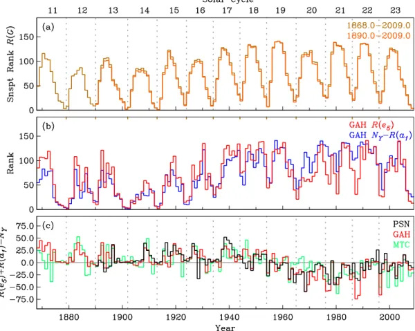
Fig. 5. Time series of ranks of(a)annual means of sunspot numbersGfor two durations of time: 1868.0–2009.0 and 1890.0–2009.0,
(b)annual residualsR(e5)−R(G), and (c)the differencesNY−R(e5)−R(a1), for German PSN, British GAH, and Australian MTC
observatory groups. In(a)–(c)the ranks of the German PSN data have been adjusted to account for their shorter duration.
statistically independent. And, indeed, as we have docu-mented in Sect. 3, PSN, GAH, and MTCKvalues are rather tightly cross-correlated. As a result, it is likely that their joint significance probability is not much smaller than 10−1; an
estimate can be obtained through a detailed bootstrap anal-ysis (not pursued). The situation, here, is analogous to that encountered in hydrology, where multiple rivers in a con-tinental region are monitored for flow-rate trends in order to estimate regional, climatological change (e.g. Lettenmaier et al., 1994). The redundant information in the threeKtime series considered here provides qualitative reassurance that their secular change has geophysical meaning. While this is important, it is also difficult to quantify with simple rank statistics.
7 Secular change and the Sun
We consider, now and in more detail, the temporal relation-ship between solar and geomagnetic activity. The Kendall coefficientsτ, measuring cross-correlation between ranks of solar-cycle-average exceedancese5and sunspot numbersG,
are PSN: 0.67, GAH: 0.74, and MTC: 0.77, where, in each case,p <10−2. These coefficients are higher than the
Pear-son coefficients measuring linear trends, Sect. 4, and higher than the Mann-Kendall coefficients measuring monotonic trends, Sect. 6, and so, as an hypothesis test, we might rea-sonably reject simple trend parameterizations in favor of a sunspot-number parameterization. This does not contradict our observation that geomagnetic disturbance has shown an increase over the past 141 years. It just means that geomag-netic activity has changed over time in a way that is neither particularly linear nor particularly monotonic. Like the solar activity that drives it, geomagnetic activity has had a complex evolution.
Details of this evolution are important. In Fig. 5b we plot, for each observatory group, residual differences between ranks of exceedances and sunspot numbers R(e5)−R(G),
and in Fig. 5c we plot residual differences between ranks of complementary attainmeents and sunspot numbersNY− R(a1)−R(G). Clearly seen is the well-known lag of a year
260 J. J. Love: Secular trends in storm-level geomagnetic activity
Fig. 6. Time series of ranks of(a)annual means of sunspot numbersGfor two durations of time: 1868.0–2009.0 and 1890.0–2009.0,
(b)annual exceedancesR(e5)and the complements of annual attainmentsNY−R(a1), for the British GAH observatory group, and(c)the
differencesR(e5)+R(a1)−NY, for German PSN, British GAH, and Australian MTC observatory groups. In(a)–(c)the ranks of the German
PSN data have been adjusted to account for their shorter duration.
geoeffective during the declining phase of the solar cycle, just after solar maximum (e.g. Legrand and Simon, 1989; Richardson et al., 2002b). But also seen, here, is the emer-gence of this lag after cycle 13 (Bartels, 1932, Sect. 14; Kishcha et al., 1999, Fig. 9; Echer et al., 2004, Fig. 2), an interesting observation that is not, perhaps, as widely ap-preciated as it should be. It demonstrates that the relation-ship between sunspot number and geomagnetic activity has changed over time. This should be regarded as cause for caution in making linear extrapolations of parameterizations of recent solar-terrestrial interaction, either forward or back-ward in time.
Over the past 141 years, the shapes of theK-index distri-butions for all three observatory groups have changed. As an example of this, in Fig. 6b we compare ranks of British GAH exceedancesR(e5)and the corresponding ranks of
comple-mentary attainments NY−R(a1). Although there is
sub-stantial correlation between these two time series, as would be expected, close inspection also shows that before (after) 1954, or the start of solar cycle 19, theNY−R(a1)are
sys-tematically lower (higher) thanR(e5), an observation that is
consistent with those based on theaa index (e.g. Legrand and Simon, 1989, Fig. 6; and Ouattara et al., 2009, Fig. 4). In Fig. 6c, we plot the differences between the two time se-ries shown in Fig. 6b, but for all three observatory groups, R(e5)+R(a1)−NY. After averaging over each solar cy-cle, the Mann-Kendall coefficientsτindicate the presence of a long-term trend, PSN: 0.42, GAH: 0.49, and MTC: 0.43, where, in each case,p <10−1. In the evolution of
geomag-netic activity, the quiescent attainmentsa1have been
dimin-ishing faster than magnetic activitye5 has been increasing.
8 Conclusions
While we can conclude that geomagnetic activity has in-creased, as a “trend”, over the past 141 years, the detailed evolution of geomagnetic activity since 1868.0 is not well-described as being approximately linear, nor, even, mono-tonic. Since geomagnetic activity is controlled by the Sun and its solar wind, a physics-based parameterization of the evolution geomagnetic activity should be tied to heliophys-ical parameters. Over the past 141 years, the only directly-measured heliophysical parameter available is sunspot num-ber, and this too has shown secular change. Given these ob-servations, and the understanding that solar-terrestrial inter-action is generally “non-linear”, it is, perhaps, not surpris-ing that the relationship between sunspot number and ge-omagnetic activity has evolved; since solar cycle 14, geo-magnetic activity has lagged behind sunspot number by a year or two, but before then the phase-lag was not very pro-nounced. Apparently, the nature of solar-terrestrial interac-tion has changed over time. Therefore, predicting the long-term future of geomagnetic activity is bound to remain diffi-cult if not impossible.
Acknowledgements. We acknowledge Intermagnet for facilitating the dissemination of magnetic observatory data and for promoting high standards of magnetic observatory practice (www.intermagnet. org). We thank E. Clarke, P. G. Crosthwaite, A. M. Lewis, H.-J. Linthe, and E. A. McWhirter for help with historical data. We thank A. Chulliat, K. Mursula, D. M. Perkins, L. Svalgaard, and V. C. Tsai for useful conversations. We thank N. L. Farr, C. A. Finn, J. L. Gannon, M. C. Nair, and Anonymous for reviewing a draft manuscript.
Topical Editor I. A. Daglis thanks A. Rodger and I. Richardson for their help in evaluating this paper.
References
Bartels, J.: Terrestrial-magnetic activity and its relations to solar phenomena, Terr. Magn. Atmos. Electr., 37, 1–52, 1932. Bartels, J.: Discussion of time-variations of geomagnetic activity
indicesKpandAp, 1932–1961, Ann. Geophys., 19, 1–20, 1963. Bartels, J., Heck, N. H., and Johnston, H. F.: The three-hour range index measuring geomagnetic activity, Terr. Magn. Atmos. Electr., 44, 411–454, 1939.
Bartels, J., Heck, N. H., and Johnston, H. F.: Geomagnetic three-hour-range indices for the years 1938 and 1939, Terr. Magn. At-mos. Electr., 45, 309–337, 1940.
Bucha, V. and Bucha, V.: Geomagnetic forcing of changes in cli-mate and in the atmospheric circulation, J. Atmos. Solar-Terr. Phys., 60, 145–169, 1998.
Cairncross, A.: Economic forecasting, Econ. J., 79, 797–812, 1969. Clilverd, M. A., Clark, T. D. G., Clarke, E., and Rishbeth, H.: In-creased magnetic storm activity from 1868 to 1995, J. Atmos. Solar-Terr. Physics, 60, 1047–1056, 1998.
Clilverd, M. A., Clark, T. D. G., Clarke, E., Rishbeth, H., and Ulich, T.: The causes of long-term change in theaaindex, J. Geophys. Res., 107, 1441, doi:10.1029/2001JA000501, 2002.
Clilverd, M. A., Clarke, E., Ulich, T., Linthe, J., and Rishbeth, H.: Reconstructing the long-termaaindex, J. Geophys. Res., 110, A07205, doi:10.1029/2004JA010762, 2005.
Cohn, T. A. and Lins, H. F.: Nature’s style: Naturally trendy, Geo-phys. Res. Lett., 32, L23402, doi:10.1029/2005GL024476, 2005. Courtillot, V., Gallet, Y., Le Mou¨el, J. L., Fluteau, F., and Genevey, A.: Are there connections between the Earth’s magnetic field and climate?, Earth Planet. Sci. Lett., 253, 328–339, 2007.
Dagum, C. and Dagum, E. B.: Trend, in: Encyclopedia of Statistical Sciences, edited by: Kotz, S., Johnson, N. L., and Read, C. B., vol. 9, pp. 321–324, John Wiley & Sons, New York, NY, 1988. Delouis, H. and Mayaud, P. N.: Spectral analysis of the
geomag-netic activity indexaaover a 103-year interval, J. Geophys. Res., 80, 4681–4688, 1975.
Echer, E., Gonzalez, W. D., Gonzalez, A. L. C., Prestes, A., Vieira, L. E. A., Lago, A. D., Guarnieri, F. L., and Schuch, N. J.: Long-term correlation between solar and geomagnetic activity, J. At-mos. Solar-Terr. Phys., 66, 1019–1025, 2004.
Ferguson, G. A.: Nonparametric Trend Analysis, McGill Univ. Press, 1965.
Feynman, J. and Crooker, N. U.: The solar wind at the turn of the century, Nature, 275, 626–627, 1978.
Feynman, J. and Gu, X. Y.: Prediction of geomagnetic activity on time scales of one to ten years, Rev. Geophys., 24, 650–666, 1986.
Finch, I. D., Lockwood, M. L., and Rouillard, A. P.: Ef-fects of solar wind magnetosphere coupling recorded at dif-ferent geomagnetic latitudes: Separation of directly-driven and storage/release systems, Geophys. Res. Lett., 35, 1L21105, doi:10.1029/2008GL035399, 2008.
Friis-Christensen, E.: Solar variability and climate – A summary, Space Sci. Rev., 94, 411–421, 2000.
Hathaway, D. H.: Does the current minimum validate (or invali-date) cycle prediction methods?, in: SOHO-23: Understanding a Peculiar Solar Minimum, edited by: Cranmer, S. R., Hoeksema, J. T., and Kohl, J. L., pp. 307–314, Astron. Soc. Pacific Confer-ence Series, 2010.
Hathaway, D. H., Wilson, R. M., and Reichmann, E. J.: Group sunspot number: Sunspot cycle characteristics, Solar Phys., 211, 357–370, 2002.
Helsel, D. R. and Hirsch, R. M. (Eds.): Statistical Methods in Water Resources, Elsevier Science Publishers, Amsterdam, The Netherlands, 1992.
Hipel, K. W. and McLeod, A. I.: Time Series Modelling of Water Resources and Environmental Systems, Elsevier Science, New York, NY, 1994.
Hoyt, D. V. and Schatten, K. H.: Group sunspot numbers: A new solar activity reconstruction, Solar Phys., 181, 491–512, 1998. Jankowski, J. and Sucksdorff, C.: Guide for Magnetic
Measure-ments and Observatory Practice, IAGA, Warsaw, Poland, 1996. Kane, R. P.: Some implications using the group sunspot number
reconstruction, Solar Phys., 205, 383–401, 2002.
Kishcha, P. V., Dmitrieva, I. V., and Obridko, V. N.: Long-term variations of the solar-geomagnetic correlation, total solar irradi-ance, and northern hemispheric temperature (1868-1997), J. At-mos. Solar-Terr. Phys., 61, 799–808, 1999.
Koutsoyiannis, D.: Nonstationarity versus scaling in hydrology, J. Hydrology, 324, 239–254, 2006.
262 J. J. Love: Secular trends in storm-level geomagnetic activity
geomagnetic storms, Ann. Geophys., 10, 683–689, 1992. Legrand, J. P. and Simon, P. A.: Solar cycle and geomagnetic
activity: A review for geophysicists. Part I. The contributions to geomagnetic activity of shock waves and of the solar wind, Ann. Geophys., 6, 565–578, 1989.
Lettenmaier, D. P., Wood, E. F., and Wallis, J. R.: Hydro-climatological trends in the continental United States, 1948–88, J. Climate, 7, 586–607, 1994.
Lockwood, M., Stamper, R., and Wild, M. N.: A doubling of the Sun’s coronal magnetic field during the past 100 years, Nature, 399, 437–439, 1999.
Love, J. J.: Magnetic monitoring of Earth and space, Physics Today, 61, 31–37, 2008.
Lukianova, R., Alekseev, G., and Mursula, K.: Effects of sta-tion relocasta-tion in theaaindex, J. Geophys. Res., 114, A02105, doi:10.1029/2008JA013824, 2009.
Luterbacher, J., Dietrich, D., Xoplaki, E., Grosjean, M., and Wan-ner, H.: European seasonal and annual temperature variability, trends, and extremes since 1500, Science, 303, 1499–1503, 2004. Macmillan, S.: Observatories, overview, in: Encyclopedia of Ge-omagnetism and PaleGe-omagnetism, edited by: Gubbins, D. and Herrero-Bervera, E., pp. 708–711, Springer-Verlag, New York, NY, 2007.
Mayaud, P. N.: IndiciesKn, Ks, Km, 1964-1967, CNRS, Paris, France, 1968.
Mayaud, P. N.: A hundred year series of geomagnetic data, 1868– 1967, indicesaa, Storm sudden commencements, IAGA Bull., 33, 1–252, 1973.
Mayaud, P. N.: Derivation, Meaning, and Use of Geomagnetic In-dices, Geophysical Monograph 22, Am. Geophys. Union, Wash-ington, D.C., 1980.
McCracken, K. G.: Geomagnetic and atmospheric effects upon the cosmogenic10Be observed in polar ice, J. Geophys. Res., 109, A04101, doi:10.1029/2003JA010060, 2004.
Mursula, K. and Martini, D.: Centennial increase in geomagnetic activity: Latitudinal differences and global estimates, J. Geo-phys. Res., 111, A08209, doi:10.1029/2005JA011549, 2006. Mursula, K. and Martini, D.: A new verifiable measure of
centennial geomagnetic activity: Modifying the K index method for hourly data, Geophys. Res. Lett., 34, L22107, doi:10.1029/2007GL031123, 2007.
Mursula, K., Martini, D., and Karinen, A.: Did open solar magnetic field increase during the last 100 years? A reanalysis of geomag-netic activity, Solar Phys., 224, 85–94, 2004.
Mursula, K., Usoskin, I., and Yakovchouk, O.: Does sunspot num-ber calibration by the “mangetic needle” make sense?, J. Atmos. Solar-Terr. Phys., 71, 1717–1726, 2009.
Oler, C.: ImperfectKindex satisfactory for electric power industry, Space Weather, 2, S06001, doi:10.1029/2004SW000 083, 2004. Ouattara, F., Amory-Mazaudier, C., Menvielle, M., Simon, P., and
Legrand, J.-P.: On the long term change in the geomagnetic ac-tivity during the 20th century, Ann. Geophys., 27, 2045–2051, doi:10.5194/angeo-27-2045-2009, 2009.
Percival, D. B. and Rothrock, D. A.: “Eyeballing” trends in climate time series: A cautionary note, J. Climate, 18, 886–891, 2005. Preece, D. A.: The language of size, quantity and comparison, The
Statistician, 36, 45–54, 1987.
Press, W. H., Teukolsky, S. A., Vetterling, W. T., and Flannery, B. P.: Numerical Recipes, Cambridge Univ. Press, Cambridge, UK, 1992.
Rangarajan, G. K.: Indices of geomagnetic activity, in: Geomag-netism, Volume 3, edited by Jacobs, J. A., pp. 323–384, Aca-demic Press, London, UK, 1989.
Rangarajan, G. K. and Barreto, L. M.: Use ofKpindex of geomag-netic activity in the forecast of solar activity, Earth Planets Space, 51, 363–372, 1999.
Rangarajan, G. K. and Iyemori, T.: Time variations of geomagnetic activity indices Kp and Ap: an update, Ann. Geophys., 15, 1271– 1290, doi:10.1007/s00585-997-1271-z, 1997.
Richardson, I. G., Cliver, E. W., and Cane, H. V.: Long-term trends in interplanetary magnetic field strength and solar wind struc-ture during the twentieth century, J. Geophy. Res., 107, 1304, doi:10.1029/2001JA000507, 2002a.
Richardson, I. G., Cliver, E. W., and Cane, H. V.: Sources of geo-magnetic activity during nearly three solar cycles (1972–2000), J. Geophys. Res., 107, 1187, doi:10.1029/2001JA000504, 2002b. Schatten, K. H. and Wilcox, J. M.: Response of the geomagnetic ac-tivity indexKpto the interplanetary magnetic field, J. Geophys. Res., 72, 5185–5191, 1967.
Stamper, R., Lockwood, M., Wild, M. N., and Clark, T. D. G.: So-lar causes of the long-term increase in geomagnetic activity, J. Geophys. Res., 104, 28325–28342, 1999.
Stuiver, M. and Quay, P. D.: Changes in atmospheric carbon-14 attributed to a variable Sun, Science, 207, 11–19, 1980. Svalgaard, L.: Calibrating the sunspot sumber using “the magnetic
needle”, CAWSES Newsletter, 4, 6–8, 2007.
Svalgaard, L. and Cliver, E. W.: Long-term geomagnetic indices and their use in inferring solar wind parameters in the past, Adv. Space Res., 40, 1112–1120, 2007.
Svalgaard, L., Cliver, E. W., and Sager, P. L.: IHV: A new long-term geomagnetic index, Adv. Space Res., 34, 436–439, 2004. Vennerstroem, S.: Long-term rise in geomagnetic activity – A close
connection between quiet days and storms, Geophys. Res. Lett., 27, 69–72, 2000.
von Storch, H.: Misuses of statistical analysis in climate research, in: Analysis of Climate Variability: Applications and Statistical Techniques, edited by: von Storch, H. and Navarra, A., pp. 11– 25, Springer-Verlag, New York NY, 1995.
Weatherhead, E. C., Reinsel, G. C., Tiao, G. C., Meng, X. L., Choi, D., Cheang, W. K., Keller, T., DeLuisi, J., Wuebbles, D. J., Kerr, J. B., Miller, A. J., Oltmans, S. J., and Frederick, J. E.: Fac-tors affecting the detection of trends: Statistical considerations and applications to environmental data, J. Geophys. Res., 103, 17149–17161, 1998.
Welling, D. T.: The long-term effects of space weather on satellite operations, Ann. Geophys., 28, 1361–1367, doi:10.5194/angeo-28-1361-2010, 2010.
Wolf, R.: Astronomische Mittheilungen, Eide¨ossischen Sternwarte Z¨urich, no. 38, 375–405, 1875.