Federal University of Minas Gerais
School of Engineering
Department of Production Engineering
Graduate Program in Production Engineering
A Network Approach to Deal with the Problem of
Examinee Choice under Item Response Theory
Thesis submitted by
Carolina Silva Pena
Under supervision of
Prof. Marcelo Azevedo Costa
In Partial Fulfillment of the Requirements for the Degree of
Doctor of Philosophy in Production Engineering
Pena, Carolina Silva.
P397n A network approach to deal whit the problem of examinee choice under item response theory [manuscrito] / Carolina Silva Pena. – 2016. ix, 75 f., enc.: il.
Orientador: Marcelo Azevedo Costa.
Tese (doutorado) - Universidade Federal de Minas Gerais, Escola de Engenharia.
Bibliografia: f. 69-75.
1. Engenharia de produção - Teses. 2. PERT (Análise de redes) - Teses. 3. Teoria da resposta do item - Teses. 4. Teoria bayesiana de decisão estatística I. Costa, Marcelo Azevedo. II. Universidade Federal de Minas Gerais. Escola de Engenharia. III. Título.
ii
Acknowledgments
I would like to express my gratitude to Professor Marcelo Azevedo Costa, who was my Academic Advisor during the masters' degree and now in the doctorate program. He revised my project several times, gave me valuable suggestions and, above all, helped me to develop as a researcher. I realized my evolution during the writing of the second paper. The first paper was very difficult to me, mainly because of the language barrier and the several rules to be addressed during the submission process. The second paper flowed much more naturally. I can say that Professor Marcelo taught me how to write a manuscript for a top international journal.
I would like to thank my beloved husband, Rivert, for encouraging me many times during this academic journey and also for valuable contributions, in the second paper, with his experience in Bayesian modeling. My special thanks to my beloved family, my mother Dora, my father Deusdedit and my brothers Guilherme and Will. After all, they have always stood by me in this world, which provided me confidence to achieve this academic degree. I dedicate this work to my friends and family.
iii
Resumo
Em uma situação típica de avaliação utilizando questões de prova, os candidatos não podem escolher quais itens preferem responder. A principal razão é um problema técnico em se obter estimativas confiáveis para as habilidades dos candidatos e as dificuldades dos itens. Este trabalho propõe uma nova representação dos dados utilizando análise de redes. As questões de prova, e os itens selecionados, para cada candidato, são codificados como camadas, vértices e arestas em uma rede multicamadas. Dessa forma, um novo modelo de Teoria de Resposta ao Item (TRI), que incorpora a informação obtida a partir da rede multicamadas utilizando modelagem Bayesiana, é proposto. Diversos estudos de simulação, nos quais os candidatos podem escolher um subconjunto de itens, foram realizados. Os resultados mostram uma melhora substancial na recuperação dos parâmetros utilizando o modelo proposto em comparação ao modelo convencional de TRI. Este modelo é a primeira proposta que permite obter estimativas satisfatórias em cenários críticos reportados na literatura.
iv
Abstract
In a typical questionnaire testing situation, the examinees are not allowed to choose which items they would rather answer. The main reason is a technical issue in obtaining satisfactory statistical estimates of examinees' abilities and items' difficulties. This paper introduces a new Item Response Theory (IRT) model that incorporates information from a novel representation of the questionnaire data, using network analysis. The questionnaire data set is coded as layers, the items are coded as nodes and the selected items are connected by edges. The new proposed Item Response Theory (IRT) model incorporates network information using Bayesian estimation. Several simulation studies in which examinees are allowed to select a subset of items were performed. Results show substantial improvements in the parameters' recovery over the standard model. To the best of our knowledge, this is the first proposal to obtaining satisfactory IRT statistical estimates in some critical scenarios reported in literature.
v
Summary
1. Introduction ... 1
2. A Network Approach to Evaluate the Problem of Examinee Choice under Item Response Theory... 3
Abstract ... 3
Introduction ... 3
Material and Methods ... 7
Network Aggregation ... 8
Centrality Measures ... 12
Multilayer Network Statistical Independence Test ... 14
Fundamentals of Item Response Theory ... 14
Simulation Study ... 17
Case Studies ... 21
Results ... 23
Case Studies ... 34
Discussion and Conclusion ... 37
Acknowledgments ... 39
3. A New Item Response Theory Model to Adjust Data Allowing Examinee Choice ... 40
Abstract ... 40
Introduction ... 40
Material and Methods ... 42
The Standard IRT Model ... 42
Inference under Examinee Choice Design... 44
Network Information ... 46
vi
Simulation Study ... 50
Results ... 52
Empirical Validation of the Proposed Model ... 52
Accuracy of the Estimated Parameters ... 56
Discussion and Conclusion ... 65
Appendix ... 67
vii
List of Figures
2.1 Network representation of selected items from a questionnaire with 20 items ... 7
2.2 Network aggregation.. ... 12
2.3 Boxplots of the simulated densities for different values of weight.. ... 24
2.4 HPD intervals for Pearson linear correlation coefficient between simulated difficulties and centrality measures using matrix O for different weight values – Scenario 1 ... 27
2.5 HPD intervals for Pearson linear correlation coefficient between simulated difficulties and centrality measures using matrix U for different weight values – Scenario 1. ... 28
2.6 HPD intervals for Pearson linear correlation coefficient between simulated difficulties and centrality measures using matrix O for different weight values – Scenario 2. ... 29
2.7 HPD intervals for Pearson linear correlation coefficient between simulated difficulties and centrality measures using matrix U for different weight values – Scenario 2. ... 30
2.8 HPD intervals for Pearson linear correlation coefficient between simulated difficulties and centrality measures using matrix O for different weight values – Scenario 3. ... 31
2.9 HPD intervals for Pearson linear correlation coefficient between simulated difficulties and centrality measures using matrix U for different weight values – Scenario 3. ... 32
2.10 Bias of estimated item difficulty versus eigenvector centrality measure, using matrix O, for simulated scenario 1. ... 34
2.11 School of engineering network. ... 35
2.12 The Brazilian lottery network. ... 37
3.1 Residual Sum of Squares versus density of matrix U. ... 54
3.2 Item difficulty versus the first eigenvector of matrix O. ... 56
3.3 Estimates minus true items' difficulties plotted against true items' difficulties for three simulated data sets.. ... 58
viii
ix
List of Tables
2.1 Summary of the main features of the three simulated scenarios ... 20
2.2 Pearson linear correlation coefficient between estimated difficulties and eigenvector centrality measures; and between estimated difficulties and strength centrality measures. ... 36
3.1 Summary of Residual Sum of Squares ... 53
3.2 The proposed values for the variance of the prior distribution ... 55
3.3 Summary of estimated parameters in scenario 1 ... 60
3.4 Summary of parameters recovery in scenario 2 ... 62
3.5 Summary of parameters recovery in scenario 3 ... 63
3.6 BUGS code for the standard Rasch Model ... 67
1
Chapter 1
1.
Introduction
One important challenge faced by large scale tests is to provide comparability between examinees performance, particularly in assessment situations in which it is not possible to apply the same test for them all. Furthermore, the comparability of the examinees performance over the years is crucial for evaluating the educational system. This problem has been overcome by estimating the examinees abilities using a set of statistical models that compose the Item Response Theory (IRT). This property, knowing as invariance, is obtained in IRT models by introducing separate parameters for examinees and items. The IRT models provides optimal estimates when all items within a test are mandatory to the examinees. On the other hand, if the examinees are allowed to choose a subset of items, instead of answer them all, the model estimates can became seriously biased. As a consequence, examinees typically are not allowed to choose which items they would rather answer.
2
3
Chapter 2
2.
A Network Approach to Evaluate the Problem of
Examinee Choice under Item Response Theory
Abstract
Item Response Theory (IRT) models are widely applied to estimate examinee ability and item difficulty using questionnaire data. However, if examinees are allowed to choose fewer items in the questionnaire then statistical estimates of parameters can be biased. This is because the choice may depend on the examinee personal ability and on the item difficulty. In this work, we explore a novel representation of examinees and their selected items using a multilayer network: the questionnaire data is coded as layers, nodes and edges. Using the multilayer network, we propose a statistical method to create a monolayer network from which network centrality measures are calculated. Simulated and real case data sets show that the estimated centrality measures are strongly and statistically correlated to item difficulty. In addition, we propose a statistical inference test to determine if the examinees are randomly selecting items. Findings are currently being investigated to minimize statistical bias in IRT estimates.
Keywords: Network analysis, Network aggregation, Centrality measures, Item Response Theory, Examinee Choice, Missing data.
4
This study analyzes the problem of evaluating individuals (or examinees) in a specific field of interest using a questionnaire or test. The test has items and for each item each individual must provide a response. After evaluating the completed test, a value is given to each item. Let be the random variable of interest that represents the value for each item ( = 1, … , ) and examinee ( = 1, … , ). If the responses of the examinees are correct then = 1, otherwise = 0. Classical Test Theory uses the number of correct responses,
∑ , to estimate the examinee ability. However, this approach does not take into account the fact that different items have different levels of difficulty [Hambleton, Swaminathan and Rogers, 1991]. For example, suppose two examinees achieve the same number of correct responses but the subset of items answered by the first examinee are, in general, more difficult. In this example, the first examinee has a superior ability which is not identified only by using the number of correct items. In practice, the examinee ability, hereafter identified as , and the item difficulty, hereafter identified as , are not known in advance. They must be estimated using the set of responses . Item Response Theory (IRT) is the methodology which is widely used to estimate examinee ability and item difficulty [Hambleton, Swaminathan and Rogers, 1991].
5
can be used to differentiate more difficult items from less difficult items. Therefore, it is of interest to identify summary statistics which can be used to select potential mandatory subsets, and which are potentially correlated to the difficulties of the items.
In this work, we explore a novel representation of the examinees and their selected items using a multilayer network. Each examinee is represented as a single-layer network in which the total number of items are the vertices, or nodes, and the selected items are fully connected by edges. That is, each edge connects pairs of items chosen by the examinee. Therefore, each layer of the multilayer network represents one examinee and the selected items. This novel representation may show relationships among the examinees and items which are not identified using only frequency of selection.
Many systems can be seen as networks or multilayer networks. For example, social networks [Verbrugge, 1979; Barrett, Henzi and Lusseau, 2012], gene co-expression networks [Li et al., 2011], transportation networks [Cardillo et al., 2013], climate networks [Donges et al., 2011], among others [Kivelä et al., 2014]. Furthermore, a multilayer representation may include interaction between layers, generally represented as connecting edges between layers. Multilayer network analysis implies that relevant information might not be identified if the single layers were analyzed separately [Menichetti et al., 2014; Battiston, Nicosia and Latora, 2014]. On the other hand, summary statistics easily can be estimated from a monolayer network. Therefore, it is of interest to represent multilayer networks as a compact layer from which relevant information regarding the problem is obtained [De Domenico et al., 2015].
6
statistical inference procedure to test the null hypothesis that the examinees are choosing items randomly. This is a useful test for investigating whether the layers in a multilayer network are correlated [Bianconi, 2013]. Finally, the following centrality measures: betweenness, closeness, degree, eigenvector and strength are calculated using the monolayer network in order to find statistical measures which are correlated to item difficulty. Simulated and real case studies show that the proposed analysis provides relevant information about item difficulty, which potentially can be used to improve IRT estimates.
7
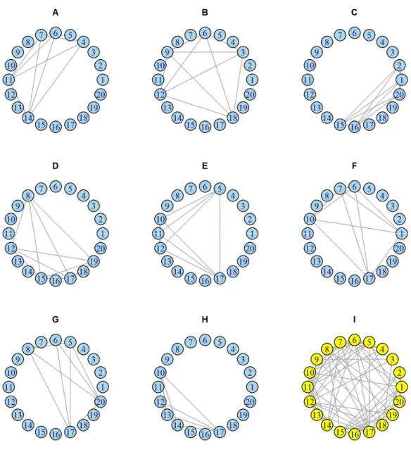
Figure 2.1:Network representation of selected items from a questionnaire with 20 items. (A-H) Represents 8 examinee networks, each with 5 selected items. In these networks, each vertex represents an item and all vertices selected by an examinee are fully connected. (I) Aggregated single-layer network in which each edge connects two items that were selected by at least one examinee.
8
Following Barrat, Barthélemy and Vespignani [2008], a network is any system that admits an abstract mathematical representation using graphs. A graph G = V, E is a collection of vertices (or nodes) which identifies the elements of a particular system and a set of edges, related to the vector . Each edge connects pairs of vertices v , v , v , v ∈
indicating the presence of a relationship or interaction between them. The maximum number of edges in network G is given by:
= ( ) , (2.1)
and its density is defined by [Lewis, 2009, p. 53]:
= . (2.2)
Network Aggregation
Consider a complex system represented using vertices and layers. Let =
( , , … , ) be a set of networks (or graphs) and is the network at layer , = 1, … , .
is also known as a multilayer network [Battiston, Nicosia and Latora, 2014]. Each network,
= , , is represented using the vector of vertices and the vector of edges . Hereafter, it is assumed that the set of vertices is the same for every layer , while the set of edges depends on each layer.
Each network can be represented using an adjacency squared matrix [ ] of dimension
where [ ] = 1 if there is an edge between vertices and in layer , and [ ] = 0, otherwise. Suppose each layer has selected vertices (0 < ≤ ), which are fully connected by edges. Thus, the sum of the total number of edges present in the multilayer network is:
9
The simplest way to aggregate multiple layers is using aggregation matrices. For instance, let be the aggregation matrix = [ ] , where:
= 1, ∃ : [ ]= 1;
0, ℎ . (2.4)
That is, pairs of vertices in matrix are connected if there is, at least, one layer in which vertices v and v are connected ( [ ]= 1) [Battiston, Nicosia and Latora, 2014]. Therefore, matrix is a summary matrix of the multilayer G which ignores multi-ties between pairs of nodes among layers.
The overlapping matrix = [ ] is an alternative aggregation matrix in which the multi-ties between pairs of nodes are not ignored [Battiston, Nicosia and Latora, 2014; Bianconi, 2013; Barigozzi, Fagiolo and Garlaschelli, 2010]:
= ∑ [ ], (2.5)
therefore 0 ≤ ≤ ∀ , . The overlapping matrix preserves the number of layers in which the connections are present as compared to matrix . Nevertheless, matrices and do not provide additional information about the existence of connections between layers, i.e., the inter-layer edges [Battiston, Nicosia and Latora, 2014].
10
= 1,0, ℎ> Ψ; ≠ ;. (2.6)
where is given by equation 2.5 and Ψis a critical upper bound value which is estimated under the null hypothesis ( ) that the multilayer is independent. Let be the random variable of interest. It represents the number of times one edge between vertex v (hereafter known as vertex ) and vertex v (hereafter known as vertex ) is observed in the multilayer . Under the null hypothesis that the multilayer is independent, it can be shown that the expected number of times that one edge connecting vertices and happens in a multilayer is:
= [ ]. (2.7)
The aggregation matrix assumes that = 1 if there is evidence that the null hypothesis is rejected, or > . It is straightforward to show that:
> → > [ ] → [ ]> . (2.8)
Alternatively, let be a random variable defined as = [ ]. is the proportion of
connections between vertices and among the sum of the total number of edges of the multilayer. Therefore, the null and alternative hypothesis are written as:
: = ,
: > . (2.9)
11
> [ ]+ [ ](1 − ) (2.10)
where is z-score statistic. For example, if = 0.05 (5%) then = 1.645. Therefore, given
, Ψ = [ ]+ [ ](1 − ). Alternativelly, Ψ is the upper bound of the observed number
of edges between vertices and if [ ] edges were randomly distributed among the layers in
the multilayer . It is worth mentioning that, under the null hypothesis, the statistical distribution of the number of incident edges in each vertex is the same for all vertices in the network. Consequently, the threshold is the same for all vertices. Thus, the proposed aggregation matrix is a summary matrix in which vertices and are connected if the observed number of edges between vertices and in the multilayer is statistically significant.
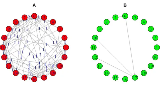
Figure 2.2A shows the overlapping network , which is represented by matrix and Figure 2.2B the statistically significant network , which is represented by matrix . The simulated data was previously used in Figure 2.1. The value of Ψ was estimated as 1.49, using
12
Figure 2.2: Network aggregation. (A) The overlapping network represented by matrix O. (B) The statistically significant network represented by matrix U.
Centrality Measures
As previously shown, the elements of the adjacency matrix represent edges which are statistically proven to be non-random. This connecting structure among vertices can be further used to identify those which are the most connected. In our proposed questionnaire network representation, statistical measures of connections among vertices, known as centrality measures, are used to identify important vertices.
Some of the most frequently used centrality measures found in the literature [Batool and Niazi, 2014] include: betweenness centrality, closeness centrality, degree centrality, eigenvector centrality and strength centrality [Barrat et al., 2004]. The first three measures were proposed by Freeman [1978] and the eigenvector centrality was proposed by Bonacich [1972].
13
= ∑ , (2.11)
where ∈ {0,1}.
The closeness centrality measure of vertex , shown in equation 2.12, is the inverse of the sum of the distances from vertex to all vertices in the network. The distance between two vertices and , , is the number of edges in the shortest path to reach vertex starting from vertex .
=∑ . (2.12)
If there is no path between two vertices (i. e., = ∞) the total number of vertices is generally used as the distance [Csardi and Nepusz, 2006].
The betweenness centrality of vertex is the number of times the vertex is found in the shortest paths between two other vertices. Let be the total number of shortest paths between vertices ℎ and , then ( ) is the number of those paths that include vertex . The betweenness centrality of vertex is:
= ∑ ( ) . (2.13)
The eigenvector centrality of vertex is the -th element of the first eigenvector of the adjacency matrix ,
= , (2.14)
14
The strength of a vertex , given the overlapping matrix O, is the sum of the weights of all the edges incident on a vertex :
= ∑ . (2.15)
Multilayer Network Statistical Independence Test
The edges represented in matrix rejected the null hypothesis shown in equation 2.9. Given statistical significance level , a certain number of the edges will reject the null hypothesis even if the null hypothesis is true. This is known as the error type I [Casella and Berger, 2002, p. 382 - 383]. Therefore, given the number of edges in matrix , we propose a global statistical test using the number of edges of matrix or, similarly, the density of matrix defined in equation 2.2. A Monte Carlo inference is proposed [Kroese, Taimre and Botev, 2011, p. 281- 343].
Under the null hypothesis that the multilayer is independent and given the total number of edges in each layer, a multilayer network is simulated by randomly connecting pairs of vertices in each layer. Then, matrix and its density are estimated. This procedure is repeated times, say = 10,000, to generate an empirical distribution of = , … , , .
The final p-value is calculated as the proportion of simulated densities greater than the observed density ( ):
= ∑ , ( ≥ )⁄10,000 (2.16)
where ( ≥ ) = 1 if ≥ and 0, otherwise. If the p-value < , then it can be concluded that the null hypothesis is false.
15
Item Response Theory (IRT) is a psychometric theory used to evaluate data collected from a questionnaire or test. It is used to estimate the abilities of the examinees and also the difficulties of the questions (or items). The examinee ability estimated by IRT do not depend on the questionnaire, i.e., examinees estimated abilities can be compared even if different questionnaires were applied. This property, known as invariance, is one important property of IRT as compared to classical test theory [Hambleton and Swaminathan, 1985]. The invariance property is obtained by introducing statistical models with separate parameters for the examinee ability and the item difficulty [Hambleton, Swaminathan and Rogers, 1991, p. 2 - 8]. The Rasch model [Rasch, 1960] is a widely used IRT model. The item characteristic curve for the Rash model is given by [Hambleton, Swaminathan and Rogers, 1991, p. 13]:
( = 1| , ) = , (2.17)
where ( = 1| , ) is the probability model that a randomly chosen examinee with ability correctly answers item . In the Rasch model, the parameter represents the ability required for any examinee to have a 50% (0.50) chance of correctly answering item . Estimates for and in the IRT models are found using the following likelihood equation [Hambleton, Swaminathan and Rogers, 1991]:
,
= ∏
∏ ( (
= 1| , )) (1 − (
= 1| , ))
,
(2.18)where = ( , , … , ) is the vector that contains the M examinees abilities, = ( , , … , ) is the vector that contains the V difficulties of the items and is the vector of observed responses.
When allowing examinee choice, the likelihood equation includes the missing-data-indicator vector = ( , , , , … , , , … , , ) where = 1 if the examinee response
16
observed values and Y denotes the missing values. Thus, the new likelihood function, described in Bradlow and Thomas [1998], is given by:
Y , Y
,
, =
Y , Y
, ,
Y , Y
,
.
(2.19)Bradlow and Thomas [1998] showed that if the examinees are allowed to choose items then valid inference for θ and can be obtained, using equation (2.18), only if the following assumptions are applied:
Y , Y
, ,
=
Y , ,
,
(2.20)Y , ,
=
Y
.
(2.21)The first assumption (2.20) is known as the missing at random (MAR) assumption and implies that examinees are not able to distinguish items that they would usually find difficult, given their abilities. The second assumption (2.21) implies that examinees of different abilities generally do not select broadly the easier or the more difficult items. Details can be found in Bradlow and Thomas [1998]. Hereafter, it is assumed that if the examinees are not randomly selecting items then the unobserved values are not missing at random.
17
Particularly, if the IRT data is structured as aggregation networks then frequencies and correlations among items (or vertices) selected by the examinees can be represented using centrality measures. Furthermore, equation 2.6 creates the aggregation matrix whose edges were individually evaluated under the null hypothesis that the assumptions described in Bradlow and Thomas [1998] are true. That is, matrix represents the questionnaire post-processed network in which the edges represent pairs of items that rejected the null hypothesis of MAR. In addition, centrality measures can be evaluated as potential predictors of the item difficulty.
Simulated and real data sets are used to estimate the elements of matrix and to evaluate statistical correlations among the centrality measures and item difficulty.
Simulation Study
The proposed network aggregation method and the centrality measures were evaluated using three simulated scenarios. In all scenarios, there is an additional random-effect parameter for each examinee that account for the choice random-effect, hereafter known as choice parameter [Wang et al., 2012]. All scenarios have a questionnaire with 50 items
( = 1, … , 50) and 1,000 examinees ( = 1, … , 1,000). The examinees can choose 20 items. In
all scenarios, the abilities of the examinees, , and the difficulties of the items, , are generated using a normal density distribution with mean zero and variance one,
~ ( = 0; = 1) and ~ ( = 0; = 1).
18
comprises items which are easier as compared to the examinee ability, i.e., ≤ . This is the group in which the examinee has a probability higher than 0.50 to achieve a correct answer. The second group comprises items which are more difficult as compared to the examinee ability, i.e., > . In this group, the examinee has a probability lower than 0.50 to achieve a correct answer. Next, a weight value ( ) is assigned to each item. For items in group 2, the weight value is [ ] = 1; whereas, for items in group 1, the weight value varies from 1 to 2:
[ ]∈ {1, 1.1, 1.2, 1.3, … , 1.9, 2.0}. If [ ] = 1 then the MAR assumption is true; whereas, for [ ]> 1, the MAR assumption is false. For example, if [ ]= 1.1, then it can be said that the
items in group 1 have a 10% higher chance of being selected as compared to the items in group 2. For each weight value in group 1, [ ], 10,000 Monte Carlo simulations are used. Furthermore, for each Monte Carlo simulation, each examinee chooses 20 items. Selected items are generated using a multinomial probability distribution. That is, the probability of examinee selecting item is:
=∑ . (2.22)
In the second scenario (scenario 2), similarly to scenario 1, the items are divided into two groups: bellow and above the choice parameter . However in the scenario 2 the choice parameter is not fixed, it is updated after each choice made by the examinee, i. e., the choice parameter was defined as a vector , where t = 1, ..., 20. The selection of the first item is similar to scenario 1, i.e., = . Suppose the first selected item has a difficulty value of ( ). Then, = ( ) and the remaining items will be divided into two new groups
using the following rule: one item belongs to group 1 if ≤ and belongs to group 2 if
19
items are changed using the rule: one item belongs to group 1 if ≤ and belongs to group 2 if > . Thus, the probabilities of selecting new items are changed using the past selected items.
The proposed second scenario is assumed to be the more consistent with a questionnaire applied over a longer period of time. Suppose, for instance, undergraduate programs of 4 to 5 years in which an examinee (or student) may pass or fail a course (or item) in each academic semester. As the examinee passes or fails some of the items, the choice parameter is changed. Consequently, the next items (courses) are chosen based on cumulative experience. In the proposed scenario, the choice parameter is estimated using the difficulty values of the past selected items. This scenario assumes that the tendency of examinees to try harder items may increase or decrease over time.
20
and the average group difficulty. In addition to the closest group, each examinee is also more likely to choose items from adjacent groups: the closest group with either a slightly higher or slightly lower average difficulty. These three groups are hereafter named the target group. Different from scenarios 1 and 2, in which the examinees are more likely to choose the easiest items, this scenario creates groups of items from which each examinee is more likely to choose items. Each simulation uses different weights for the items in the target group,
[ ]> 1; whereas for items in the remaining groups, [ ] = 1. As a consequence, the
probability of the examinees choosing items from the target group is greater than the probability of them choosing items from the remaining groups. Similar to scenario 2, after each selected item, each choice parameter ( ) is updated using the 60% percentile of the difficulties of the previously selected items. Table 2.1 shows the main features of each simulated scenario; also, the differences between them.
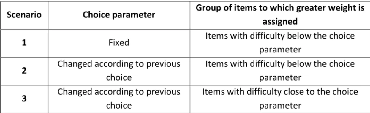
Table 2.1: Summary of the main features of the three simulated scenarios
Scenario Choice parameter Group of items to which greater weight is assigned
1 Fixed Items with difficulty below the choice parameter
2 Changed according to previous choice Items with difficulty below the choice parameter 3 Changed according to previous choice Items with difficulty close to the choice parameter
21
[ ]∈ {1, 1.5, 2.5, 5.0, 10, 20, 30, 50}. This is because, for scenario 3, convergence of the
network density was achieved for larger values of [ ], as compared to scenarios 1 and 2. The simulation study was performed using the R software [R Core Team, 2015].
Case Studies
The School of Engineer Data Set
The data set comprises 23 elective (i.e., not mandatory) subjects attended by 217 students of Control and Automation Engineering in years 2004, 2005 and 2006, at the Federal University of Minas Gerais (UFMG), Brazil. We obtained permission from the Graduate Studies Office of the Federal University of Minas Gerais to access this data set in compliance with Brazilian Law no. 12527 which states that all information produced or held in the custody of the government, except for personal or legally classified information, is public and therefore accessible to all citizens. No personal identification of the students was required, i.e., the data was de-identified.
The selected 217 students were enrolled in at least two of the 23 subjects. Most of the students attended from 6 to 12 courses. Therefore, the associated multilayer network has 217 layers, each layer represents the student network of selected courses. The total number of edges in the multilayer network ( [ ]) is 10,253. The total number of vertices, in each layer, is
23.
22
acknowledgments) sent an email to all students. Completion of the questionnaire was entirely voluntary. The data was anonymous, i.e., there was no field in the questionnaire for personal identification. Twenty four former students assigned score values to the courses. The linear correlation of median score values of the former students and the coordinator score values is 0.62. The final estimate of the difficulty level for each course is the average value of the coordinator score and the median score of the former students.
The coordinator also classified each course into one of the following groups: low relevant course, medium relevant course and high relevant course. Each group is based on the opinion of the coordinator about the course contribution to the minimum preparation of a control and automation engineer.
The Brazilian Lottery Data Set
The Mega Sena is a very popular lottery game in Brazil. It happens two times a week,
on average. The game comprises 6 numbers which are randomly selected from a group of 60 numbers: 1, 2, . . . , 60. Selected numbers from previous games are available online
(http://loterias.caixa.gov.br/wps/portal/loterias/landing/megasena). All numbers drawn in the Brazilian Lottery are obtained by clicking on the link "Resultado da Mega sena por ordem crescente" located at the bottom of the page. The data are publicly available for free download, therefore no permission was required.
We evaluated the numbers from the first game, in March 11, 1996 to game number 1,741, which happened in September 12, 2015. Therefore, the multilayer network has 1,741 layers. Each layer has a total of 60 vertices and 6 selected vertices, forming a clique. The total number of edges in the multilayer network ( [ ]) is 26,115. This data set was selected because
23
Results
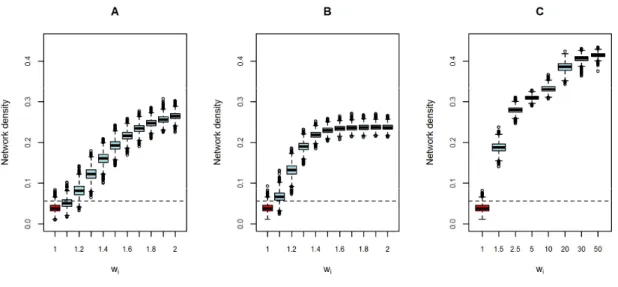
Figure 2.3 shows boxplots of the density statistic ( ) of matrix for the simulated scenarios (1, 2 and 3), for the different values of . Note that if = 1 then the MAR assumption is true. Figure 2.3 also shows a horizontal line which represents the 95th percentile
of the simulated densities for = 1. Therefore, simulations in which the density is above the horizontal line statistically reject the MAR assumption. For scenario 1, shown in Figure 2.3A, when = 1.1 the simulated density distribution was slightly different from the MAR simulated density. If > 1.1 then the simulated density distributions become much different from the MAR simulations. In general, the larger the weigth the greater the differences between simulated densities and simulated densities under the MAR assumption. Therefore, simulated results for scenario 1 show that the greater the density statistic of matrix U the more likely the examinees are choosing easier items given their personal abilities.
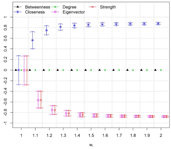
Figure 2.3B shows simulated results for scenario 2. It is worth mentioning that the results for = 1 are similar to scenario 1. The greater the value of the greater the differences between simulated densities and the MAR simulations, as similar to scenario 1. Furthermore, scenario 2 has a larger increasing rate of the distances as compared to scenario 1. For example, the median density for scenario 1 is 0.082 if = 1.2, whereas for scenario 2 the median density is 0.132 using the same value. This is because selected items are affected by previous selected items in scenario 2. At each step, when the examinee chooses an easier item, the number of items that comprises group 1 became smaller. As a consequence, the chance of choosing these fewer (and easier) items in the future is high. Thus, the network density rate is larger for scenario 2 as compared to the network density rate for scenario 1.
24
in scenarios 1 and 2. Similar to scenarios 1 and 2, the larger the values of the larger the density statistic. Furthermore, the density statistic achieved larger values before reaching convergence, as compared to scenarios 1 and 2. This is because the edges in matrix U, in scenario 3, are not concentrated toward the easiest items.
Figure 2.3: Boxplots of the simulated densities for different values of weight . (A) Scenario
1. (B) Scenario 2. (C) Scenario 3. The lower outer contour of the rectangle indicates the first quartile (Q1), the upper outer contour of the rectangle indicates the third quartile (Q3) and the horizontal line inside the rectangle indicates the median (Q2). Vertical lines extended from the box indicate variability outside the first and third quartiles. The upper vertical line indicates the maximum observed value within the range [Q3; Q3+1.5(Q3-Q1)]. The lower vertical line indicates the minimum observed value within the range [Q1; Q1-1.5(Q3-Q1)]. Observations beyond the vertical lines are represented as points and indicate outliers.
25
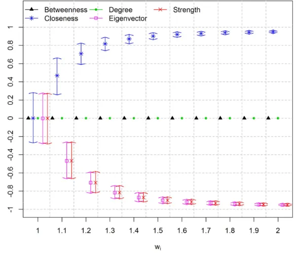
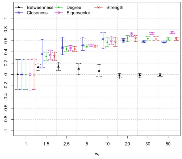
for each value. Figure 2.4, Figure 2.6 and Figure 2.8 show centrality measures calculated using matrix O. Figure 2.5, Figure 2.7 and Figure 2.9 show centrality measures calculated using matrix U. It is worth noticing that the HPD intervals are centered at zero if = 1. This is because under MAR assumption the correlation between the difficulties of the items and centrality measures are zero, on average.
Results show that the linear correlation between item difficulty and degree centrality, and between item difficulty and the betweenness centrality, using matrix O, was always zero. This is because, in all simulations, matrix O became fully connected and, consequently, both degree and betweenness centrality measures assumed the same value for all vertices. It is worth mentioning that the correlation between these two centrality measures and the difficulty of the items were set to zero because there is no correlation if one of the variables is actually a constant. In scenarios 1 and 2, the closeness centrality measure using matrix O is positively correlated to item difficulty. This is because the weights of the edges are interpreted by the algorithm as cost [Dijkstra, 1959]. Therefore, the easier items, with smaller values of , also present smaller values of closeness, and vice-versa. If matrix U is used, then the correlation is negative. This is because matrix U is binary and sparser and, as a consequence, the easiest items have larger values of closeness, and vice-versa. Furthermore, using matrix O,
26
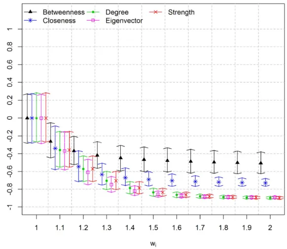
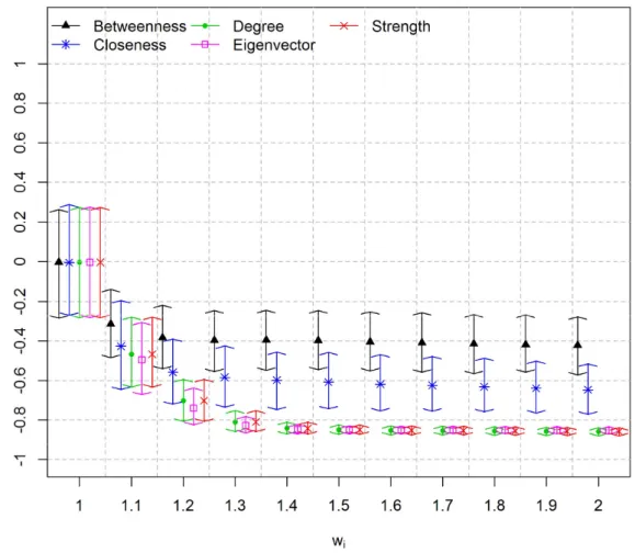
Unlike matrix O, for a larger number of examinees, matrix U does not become saturated. As a consequence, none of the evaluated centrality measures become saturated. Furthermore, the strength and degree centrality measures are similar if matrix U is used. This is because the strength centrality measure, using a non-weighted matrix, is equal to the degree centrality measure. It is worth noticing that using matrix U the closeness and betweenness centrality measures, which are related to network paths, did not correlate equally well with item difficulty as compared to degree and eigenvector centrality measures. This is because matrix U is a simplified matrix in which the edges are related to the strength of the items rather than to network internal connectivity. Therefore, no physical meaning was assigned to the distance between two items in matrix U.
In general, the eigenvector centrality measure using matrix O achieved slightly superior results as compared to matrix U for scenarios 1 and 2. This is because the easiest items are the most likely choices among the examinees in these scenarios. These items are easily detected using frequency information, which is best represented in matrix O. It is worth mentioning that matrix U is a sparser matrix carrying partial information of matrix O. Nonetheless, results using matrix U are very close to the results using matrix O. Thus, there is evidence that the information loss using matrix U is minimal.
27
centrality measures using matrix U are more correlated to item difficulty as compared to matrix O in scenario 3.
Figure 2.4: HPD intervals for Pearson linear correlation coefficient between simulated
difficulties and centrality measures using matrix O for different weight values ( ) – Scenario
28
Figure 2.5: HPD intervals for Pearson linear correlation coefficient between simulated
difficulties and centrality measures using matrix U for different weight values ( ) – Scenario
29
Figure 2.6: HPD intervals for Pearson linear correlation coefficient between simulated
difficulties and centrality measures using matrix O for different weight values ( ) – Scenario
30
Figure 2.7: HPD intervals for Pearson linear correlation coefficient between simulated
difficulties and centrality measures using matrix U for different weight values ( ) – Scenario
31
Figure 2.8: HPD intervals for Pearson linear correlation coefficient between simulated
difficulties and centrality measures using matrix O for different weight values ( ) –
32
Figure 2.9: HPD intervals for Pearson linear correlation coefficient between simulated
difficulties and centrality measures using matrix U for different weight values ( ) – Scenario
3.
33
34
Figure 2.10: Bias of estimated item difficulty versus eigenvector centrality measure, using
matrix O, for simulated scenario 1. The legend shows two groups of items: those with degree equal to zero and those with degree greater than zero, using matrix U. (A) The MAR assumption is true. (B) Weight value is 1.5. (C) Weight value is 2. (D) Weight value is 20.
Case Studies
Results: School of Engineering Data Set
35
5%. Thus, matrix has two connected subjects (or vertices) if, at least, 51 students selected the same pair of subjects. Figure 2.11B shows the final network related to matrix . The network has 17 connected vertices, or subjects. The size of the vertex represents the difficulty level of each subject, i.e., the larger the vertex, the larger the estimated difficulty score.
Figure 2.11: School of engineering network. (A) Single-layer network using the aggregation matrix . (B) Single-layer network using the aggregation matrix . Vertex size is proportional to the difficulty level of each subject. Vertex color indicates the relevance of the course to the minimum preparation of a control and automation engineer, according to the opinion of the coordinator.
The p-value, estimated using equation 2.16, is less than 0.0001 (< 10-4). Therefore,
36
In addition, the Pearson linear correlation coefficient between eigenvector centrality from matrix U and estimated difficulties; and between strength centrality from matrix O and estimated difficulties were estimated, as shown in Table 2.2. The correlation between eigenvector measures and estimated difficulties is −0.62 (p-value = 0.0015), and between strength measures and estimated difficulties is −0.57 (p-value =0.0048). For low and high relevant subjects the correlations are statistically non-significant. For high relevant subjects the difficulty does not seem to be a determining factor in the student decision, i. e., the correlation coefficient is close to zero. Furthermore, there are fewer subjects in low and high relevant subjects' groups. On the contrary, for medium relevant subjects the correlation can be considered statistically significant. This indicates that the students are selecting subjects with lower difficulties among the medium relevant subjects, as can be seen in Figure 2.11B.
Table 2.2: Pearson linear correlation coefficient between estimated difficulties and eigenvector centrality measures; and between estimated difficulties and strength centrality measures.
It is worth mentioning that the difficulty scores for the subjects were estimated independently, without fitting an IRT model. Results support the claim that centrality measures, using the proposed multilayer network approach, are statistically correlated to item difficulty.
Results: The Brazilian Lottery Data Set
Group of subjects Correlation p-value Correlation p-value Eigenvector Strength Number of subjects
all subjects -0.62 0.0015 -0.57 0.0048 23
Low relevant subjects -0.59 0.1589 -0.51 0.2382 7
Medium relevant subjects -0.87 0.0006 -0.84 0.0013 11
37
Figure 2.12A shows the overlapping network of the Brazilian lottery data set. The critical upper bound value was estimated as Ψ = 21.07, using a statistical significance level of 5%. Thus, matrix has two connected lottery numbers (or vertices) if the same pair of numbers occurred, at least, in 22 games. Figure 2.12B shows the final network related to matrix .
Figure 2.12: The Brazilian lottery network. (A) Single-layer network using the aggregation matrix . (B) Single-layer network using the aggregation matrix .
The p-value, estimated using equation 2.16, is 0.5308. Thus, there is statistical evidence that the null hypothesis of an independent multilayer network is true. That is, there is no pattern of numbers which are repeatedly being selected.
Discussion and Conclusion
38
scenario in which the examinees are allowed to choose fewer items in the questionnaire. In this situation, IRT models fail to estimate the difficulties of the items. The proposed approach creates a multilayer network using the questionnaire data. In sequence, an overlapping network, identified using matrix O, is created using the multilayer network. Statistical procedures simplify the overlapping network generating a sparser network, known as matrix
U. Centrality measures were investigated using both matrices O and U.
Results using simulated data and real case data sets show that centrality measures are strongly and statistically correlated to item difficulty. In the first and second simulated scenarios, the strength and the eigenvector centrality measures, using matrix O, are the most correlated measures to item difficulty. It is worth mentioning that the strength centrality measure using matrix O is proportional to the frequency of selected items. In the third scenario, the eigenvector centrality measure, using matrix U, is the most correlated measure to item difficulty. Nonetheless, our findings strongly suggest that the eigenvector centrality measure is the most consistent and robust statistic to estimate item difficulty, as compared to the remaining measures.
Furthermore, the proposed simplified network can be used to create a visual representation of the questionnaire, and the pairs of items which are the most frequently chosen by the examinees. This is particularly useful for educational researchers. This is illustrated using the Brazilian School of Engineering data set. It is worth noticing that the simplified network may have edges between items, even though the examinees are randomly choosing items. The proposed Monte Carlo statistical inference procedure provides a global statistical test which identifies whether the questionnaire multilayer network is independent.
39
the eigenvector centrality measure; and, linear predictors of the item difficulty, using centrality measures as independent variables.
Acknowledgments
40
Chapter 3
3.
A New Item Response Theory Model to Adjust
Data Allowing Examinee Choice
Abstract
In a typical questionnaire testing situation, the examinees are not allowed to choose which items they would rather answer. The main reason is a technical issue in obtaining satisfactory statistical estimates of examinees' abilities and items' difficulties. This paper introduces a new Item Response Theory (IRT) model that incorporates information from a novel representation of the questionnaire data, using network analysis. Three scenarios in which examinees are allowed to select a subset of items were simulated. In the first scenario, the assumptions required to apply the standard Rasch model are met, thus establishing a reference of the parameters' accuracy. The second and third scenarios include five increasing levels of violation of those assumptions. Results show substantial improvements in the parameters' recovery over the standard model. Furthermore, the accuracy was closer to the reference in almost every evaluated situation. To the best of our knowledge, this is the first proposal to obtaining satisfactory IRT statistical estimates in these two last scenarios.
Keywords: Bayesian Modeling, Examinee choice, Item Response Theory, Missing data, Network analysis, Selection of items.
41
Item response theory (IRT) comprises a set of statistical models for measuring examinees' abilities through their answers to a set of items (questionnaire). One of the most important advantages of IRT is to allow the comparison between examinees who answered to different tests. This property, known as invariance, is obtained by introducing separate parameters for the examinees' abilities and items' difficulties [Hambleton, Swaminathan and Rogers, 1991, p. 2 -8]. The IRT models have optimal properties when all items within a test are mandatory to the examinees. On the contrary, if the examinees are allowed to choose subset of items, instead of answer them all, the model estimates may became seriously biased. This problem has been raised by many researchers [Wainer, Wang and Thissen, 1994; Fitzpatrick and Yen, 1995; Wang, Wainer and Thissen, 1995; Bradlow and Thomas, 1998; Linn, Betebenner and Wheeler, 1998; Cankar, 2010; Wang et al., 2012], but still remains without a satisfactory proposal.
This is an important issue because several studies have provided evidences that choice has a positive impact in terms of educational development [Brigham, 1979; Baldwin, Magjuka and Loher, 1991; Cordova and Lepper, 1996; Siegler and Lemaire, 1997]. That is, they indicated that allowing students to choose increase the motivation and the depth of engagement in the learning process. In a testing situation, allowing choice seems to reduce the concern of examinees regarding the impact of an unfavorable topic [Jennings et al., 1999]. Besides, it has been claimed as a necessary step for the improvement of educational assessment [Rocklin, O’Donnell and Holst, 1995; Powers and Bennett, 2000].
42
are intended. Therefore, these items were pre-tested. The pre-test process is typically extremely expensive and time-consuming. For example, in 2010 was reported that the Brazilian government spent about $3.1 million to calibrate items for an important national exam (ENEM). Nevertheless, serious problems were reported to had occurred during the pre-test, like the supposedly illegal copy of many items by employees of a private high school college and their subsequent leakage. In addition, it was released that the number of items currently available in the national bank was about 6 thousand, whereas the ideal number would be between 15 and 20 thousand. All these events were harshly criticized by the mainstream media [Agência Brasil, 2010; Moura, 2010; Borges, 2011; S.P. and Mandelli, 2011]. Many recent researches have developed optimal designs for items calibration in order to reduce costs and time [Van der Linden and Ren, 2014; Lu, 2014]. Still, there is a limit for the number of items that an examinee can proper answer within a period of time. If the examinees are allowed to choose items within a total o items ( < ) and satisfactory statistical estimates are provided for all the items, the costs of calibration per item are reduced.
This paper presents a new IRT model to adjust data generated using an examinee choice allowed scenario. The proposed model incorporates, in the IRT model, network analysis information using Bayesian modeling. Results show substantial improvements in the accuracy of the estimated parameters as compared to the standard IRT model, mainly in situations in which the examinees' choice are not a random selection of items. To the best of our knowledge, this is so far the only proposal that achieved a satisfactory parameters' estimation in some scenarios reported in literature, known as very critical scenarios to the standard Rasch model estimates [Bradlow and Thomas, 1998].
Material and Methods
43
The Rasch model [Rasch, 1960] is a widely used IRT model. The item characteristic curve is given by equation 3.1 [Hambleton, Swaminathan and Rogers, 1991, p. 12]:
( = 1| , ) = , (3.1)
where Y = {0,1} is a binary variable that indicates whether examinee α correctly answered item ; is the ability parameter of examinee α; is the difficulty parameter of item ;
( = 1| , ) is the probability that a randomly chosen examinee with ability correctly
answers item and the probability of an incorrect response is equal to ( = 0| , ) =
1 − ( = 1| , ).
In the Rasch model, the parameter represents the ability required for any examinee to have a 50% (0.50) chance of correctly answering item . Given M examinees and V items, estimates for and in the IRT models are found using the likelihood showed in equation 3.2 [Hambleton, Swaminathan and Rogers, 1991, p. 41]:
, = ∏ ∏ ( ( = 1| , )) (1 − ( = 1| , )) , (3.2)
where = ( , , … , ) is the vector of the examinees' abilities, = ( , , … , ) is the vector of the items' difficulties and is the vector of the observed responses. To use Bayesian estimation, the prior distributions ( ) and ( ) must be defined. Since ⊥ , ⊥ ,
⊥ , for r ≠ s and p ≠ q, then the joint posterior distribution for parameters and is given by equation 3.3.
( , | ) ∝ ( | , ) ∏ ( ) ∏ ( ). (3.3)
44
[2010]. Furthermore, a usual prior distribution for the item parameter is given by equation 3.4 [Albert, 1992; Patz and Junker, 1999; Curtis, 2010, Fox, 2010, p. 21]:
| , ~ ( , ). (3.4)
where ( , ) denotes a normal distribution with mean of and variance of . One can use Markov Chain Monte Carlo (MCMC) methods to sample from the posterior distribution of and . Details about MCMC in the context of IRT are found in Patz and Junker [1999]. In the Appendix, a BUGS [Gilks, Thomas and Spiegelhalter, 1994] code for the adjustment of the standard Rasch model is found.
Inference under Examinee Choice Design
When allowing examinee choice, the likelihood equation includes the missing-data-indicator vector = ( , , , , … , , , … , , ), where = 1 if examinee response for
item is observed; otherwise, = 0. Given , the set of responses can be written as
= (Y , Y ) [Rubin, 1976], where Y denotes the observed values and Y denotes the
missing values. Thus, the likelihood function given in equation 3.2 is rewritten [Bradlow and Thomas, 1998] as shown in equation 3.5:
Y , Y , , = Y , Y , , Y , Y , , (3.5)
and the joint posterior distribution is given by equation 3.6:
( , , |
,
) ∝ Y , Y , , Y , Y , ∏ ( ) ∏ ( ). (3.6)45
Y , Y , , = Y , , , (3.7)
Y , , = Y . (3.8)
Assumption (3.7) is known as the missing at random (MAR) assumption and implies that examinees are not able to distinguish which items they probably would answer correctly. Assumption (3.8) implies that examinees of different abilities generally do not broadly select the easier or the more difficult items. Further details are found in Bradlow and Thomas [1998]. If both assumptions (3.7) and (3.8) hold, then the posterior distribution can be rewritten as shown in equation 3.9:
, , , ∝ , , ∏ ( ) ∏ ( ). (3.9)
In this case, it is assumed that the process that generates missing data is non-informative. Details about statistical inference in the presence of missing data are found in Rubin [1976]. Since Y is unknown, MCMC methods can be used to draw samples from the posterior distribution [Patz and Junker, 1999]. That is possible because equation 3.5 is an augmented data likelihood. Hereafter, it is assumed that if the examinees are randomly selecting items then the unobserved values are MAR; otherwise, the process that generates missing data is informative and the unobserved values are not MAR.
46
that they had made a disadvantaged choice. Moreover, the examinees who chose item 11 performed better on both items as compared to those who chose item 12. These results were observed elsewhere (Chi, 1978; Chi, Glaser and Rees, 1982), suggesting that students with higher abilities are more able to differentiate difficulties between items.
Furthermore, Bradlow and Thomas [1998] performed simulation studies to demonstrate the bias in the estimated parameter, using the standard Rasch model in violation of assumptions (3.7) and (3.8). The complete data set had 5.000 examinees and 200 items. In the simulation study, 50 items were mandatory and the remaining 150 items were divided into 75 choice pairs. In the experiment in which the first assumption (3.7) was violated, there occurred a consistent underestimation of item difficulty for the 50 mandatory items and more severe underestimation for the remaining 75 choice pairs. Furthermore, in the experiment in which the second assumption (3.8) was violated, there occurred overestimation of item difficulty for high-difficulty items and underestimation for low-difficulty items. The authors also stated that very little is known about the nature and magnitude of realistic violations of those assumptions.
Wang et al. [2012] proposed the inclusion of a random-effect parameter γ in the standard IRT models to account for the choice effect. The proposed model produced better results in some simulated scenarios as compared to the standard IRT model. Nevertheless, the authors state that if the first (3.7) or the second assumption (3.8) is violated, as described in Bradlow and Thomas [1998], valid statistical inferences are not obtained for the standard IRT model, or for the proposed model with the random-effect parameter.
Network Information
47
0 < ≤ . A novel representation of examinees and their selected items using network analysis was proposed. The data set was coded as layers, vertices (or nodes) and edges. Briefly, a network (or graph) G = V, E consists of a set of vertices (V) that identify elements of a system and a set of E edges (E) that connect pairs of vertices { , }, pointing out the presence of a relationship between the vertices [Barrat, Barthélemy and Vespignani, 2008]. In the proposed network representation, each examinee is represented as a single network in which the items are the vertices and every pair of the selected items is connected by an edge. That is, the data set is initially represented as M single-layer networks, or a multilayer network = ( , , … , ) [Battiston, Nicosia and Latora, 2014]. From the multilayer network, two matrices are created.
The first matrix, called overlapping matrix, = , is a weighted × matrix in which the elements indicate the number of examinees that chose both items and [Bianconi, 2013; Battiston, Nicosia, Latora, 2014]:
= ∑ [ ] (3.10)
where [ ] = 1 if examinee chose both items and and 0 otherwise, 0 ≤ ≤ ∀ , . The second matrix, called matrix = [ ] , is a binary × matrix in which is equal to 1 if (equation 3.10) is greater than a threshold (Ψ) and zero otherwise. The threshold is calculated to identify recurrent edges in the multilayer network and is given by equation 3.11:
Ψ = [ ]+ [ ](1 − ), (3.11)
where [ ]= ∑ ( ) is the total number of edges in the multilayer network,
48
of incident edges in each pair of vertices is the same. Thus, Ψ represents the upper bound of the observed number of edges between vertices and under the hypothesis that the [ ]
edges are randomly distributed. Further details are found in the Chapter 2 of this thesis. Therefore, matrix is a binary matrix that preserves only the statistically significant edges, as shown in equation 3.12:
= 1, > Ψ; ≠ ;
0, ℎ . (3.12)
In the Chapter 2 of this thesis, it was shown that the density of matrix U can be used to test whether the MAR assumption holds. Furthermore, the larger the density of matrix U the more violated the MAR assumption; that is, the density of matrix U indicates the violation level of the MAR assumption. The density of a network G = V, E is given in equation 3.13 [Lewis, 2009, p. 53]:
= ( ). (3.13)
Moreover, in the Chapter 2 several simulation studies using three different scenarios were performed. Several network centrality measures, and their correlations with item difficulty when MAR assumption is violated, were evaluated. Most frequently centrality measures found in literature [Batool and Niazi, 2014] were tested. The eigenvector of matrix
O was found to be the most consistent and robust network statistic to estimate item difficulty. The eigenvector centrality of a vertex ( ) is the -th element of the first eigenvector of matrix
O:
ρ = ρ (3.14)
49
correlation between the eigenvector centrality and items difficulties. It is worth mentioning that the eigenvector centrality assumes values within the range 01. Therefore, it provides a standardized measure of vertex centrality.
The Proposed Model
In general, the relation between item difficulty and first eigenvector of matrix O can be written as shown in equation 3.15.
= ( ) (3.15)
where ( ) is a function of the -th element of the first eigenvector ρ. We propose a new IRT model that takes into account the relation shown in equation 3.15. This can be achieved defining the following prior distribution:
| , ~ , , (3.16)
where = ( ) and accounts for the variability of that can not be explained by ( ). It is worth mentioning that the larger the correlation between ρ and the lower the dispersion parameter . The posterior distribution, shown in equation 3.6, can be rewritten as follows in equation 3.17:
, , ρ, , ∝ ρ, Y , Y , ,
× Y , Y ρ, , ∏ ( | ) ∏ ( ). (3.17)
If the assumptions (3.7) or (3.8) do not hold but, given ρ, the equation 3.18 holds, the proposed model can provide valid statistical inference.
50
Equation 3.18 assumes that, given ρ, the missing-data-indicator became independent of
Y , and . Further information about conditioning on covariates for missingness mechanism become ignorable are found in [Little and Rubin, 1987, p. 9 -17; Bhaskaran and Smeeth, 2014].
In this paper, the following mathematical model between ρ and is proposed:
= − log ( ( ) ) + (3.19)
where , and are coefficients, to be estimated, and C is the minimum value of , i. e.,
= min(ρ). This model represents the inverse equation of a logistic function with a changed
shape that asymptotically tends to the lowest value of ρ .The parameter is required to move the vector ρ bellow 1. Furthermore, the parameter is also used to shift vector ρ above its lowest value to prevent that log ( ) = +∞. This model was empirically proposed based on the simulation studies, shown in the Results section. It is worth mentioning that other functions to describe the relation between ρ and can be proposed. The BUGS code for the Proposed Model is available in the Appendix.
Simulation Study
51
In the first scenario, hereafter named scenario 1, both assumptions (3.7) and (3.8) were valid. That is, the items were randomly selected by the examinees and consequently the process that causes missing data was non-informative. Therefore, this is the scenario in which valid statistical inference can be obtained using the standard Rasch model.
The second scenario, named scenario 2, is identical to the first simulation scenario presented in the Chapter 2. In this scenario, each examinee chooses items based on current values of and . That is, for each examinee , the items are divided into two groups: the first group comprises items which are easier as compared to the examinee ability, i.e., ≤ . This is the group in which the examinee has a probability higher than 0.50 to achieve a correct answer. The second group comprises items which are more difficult as compared to the examinee ability, i.e., > . In this group, the examinee has a probability lower than 0.50 to answer the items correctly. A weight value ( ) is assigned to the items in each group. For items in group 2, the weight value is [ ] = 1; whereas, for items in group 1, the weight value varies from 1.5 to 30: [ ]∈ {1.5, 2, 5, 10, 30}. For example, if [ ]= 2, then it can be said that the items in group 1 have twice the chance of being selected by the examinee as compared to the items in group 2. In this scenario, assumptions (3.7) and (3.8) are violated.
52
It is worth mentioning that the selected items were generated using a multinomial probability distribution. That is, the probability of examinee selecting item is:
=∑ . (3.20)
In scenario 1, = 1 ∀ .
Results
In the Results section first we present empirical evidence of the proposed function given in equation 3.19 to describe the relation between and . Second, we define values for the variance parameter of the prior distribution ( ). Prior values of the paramater improve statistical properties of the proposed model. Finally, several simulation studies are performed in different conditions to compare the accuracy of parameters recovery obtained using the standard Rasch model and using our proposed model.
Empirical Validation of the Proposed Model
To evaluate the performance of the proposed function (equation 3.19) to predict item difficulty, using the first eigenvector of matrix O, we performed 10.000 Monte Carlo simulations for scenarios 2 and 3 and calculated the Residual Sum of Squares (RSS), shown in equation 3.21.
= ∑ ( − ) (3.21)
where is the fitted value of using equation 3.19. It is worth mentioning that the smaller the value of RSS, the better the fit of the model and the lower the bias of the estimates. The