329
L. C. Passarini and
P. R. Nakajima
Universidade de São Paulo EESC -Escola de Engenharia de São Carlos 13566-590 São Carlos, SP. Brazil [email protected]
Development of a High-Speed
Solenoid Valve: an Investigation of
the Importance of the Armature Mass
on the Dynamic Response
Traditional design criteria for electromagnetic valves are discussed. Performance criteria for them are also shown. A method for investigating the armature mass importance on the EFI performance is proposed. This method is based on energy losses of a mass-spring-damper system (MKsB). It was found a range of values in which the dynamic response can be improved. Results are verified and discussed.
Keywords: Solenoid fuel injector, mathematical model, electromagnetic actuator
Introduction
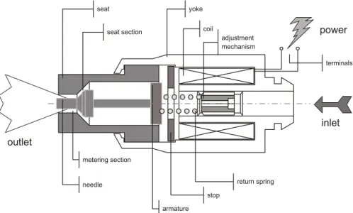
Otto Cycle engines with fuel injection systems are equipped with one or more electromagnetic fuel injectors (EFIs) mounted at the intake manifold (Fig. 1). The EFI injects the fuel into the intake valve in a way that the delivered fuel mixes with the intake air, forming the air-fuel (A/F) mixture that will be burned within the cylinders. The EFI functioning is well known and it can be explained with a little help of Fig.2. When an electrical driving command is applied to its terminals, the EFI coil is energized. Then the armature that is pressed against the valve seat is attracted by the solenoid poles and moves up against them. This movement causes an opening at the metering section where the fuel, under pressure, passes and as soon as it leaves the valve is pulverized into fine droplets. When the electrical excitation stops, the attracting force diminishes very quickly because the coil is de-energized and the armature is pushed against the valve seat by the action of the return spring, closing the fuel passage. So, it can be said that at the EFI, the released fuel per pulse Q, is a function of the electrical exciting pulse width W applied to the solenoid of the EFI.1
The dynamic response if the EFI solenoid is of primary importance. For example, an important requirement for small engines is that the EFI should present good linearity and precision under the smallest pulses, and with minimum opening and closing times. In fact, Greiner at al. (1987) affirm that linearity in the small pulses is especially important for small engines where it is demanded that fuel metering is done with high precision under the smallest pulses. These requirements have motivated to investigate the EFI design, particularly the influence of the armature mass on the EFI dynamic response, in order to find a way that meets the performance requirements and improve the EFI dynamic response. The way by which it was done was by modelling the EFI’s mechanical system and looking for clues that point to a satisfactory design.
State-of-Art of the Traditional Approaches to Designing EFIs
According to Kushida (1985), the conditions for optimization of an EFI are those that relate high-speed response and high power dissipation. That is, it is necessary to allow high energy input and to convert this into kinetic energy in an intended direction for efficiency. This is achieved by:
Paper accepted August, 2003. Technical Editor: Atila P. Silva Freire.
x a) dissipating the heat sufficiently to permit high input of electrical energy;
x b) concentrating the magnetic flux in an objective magnetic field;
x c) limiting the generated magnetic force into an objective direction and
x d) decreasing the moving mass as much as possible.
Kajima-Kamamura (1995) affirm that high speed operation can be obtained by actuating
x a) increasing the solenoid force to actuate the armature; x b) reducing the resisting force due to reactions, and/or; x c) reducing the weight of moving parts.
It can be noticed that there is little difference between Kushida’s and Kajima-Kamamura’s proposals. In this article the approach of optimizing the EFI performance by decreasing the moving mass as much as possible will be discussed and it will be demonstrated that it is not completely true since it is possible to find a particular moving mass that permit a high performance without necessarily being the smallest possible.
Subsidies for an Analysis of the EFI ’s Performance:
In order to evaluate and to compare the results better, it becomes opportune to present some of the criteria generally adopted when analyzing the EFI performance. Those criteria were defined by the EFI makers and by the designers of engine electronic control systems. The main criteria and those that are the most relevant for this article are these: static flow, dynamic flow, calibration, linearity and dynamic range.
According to DeGrace-Bata (1985), the static flow, also called full opening, is achieved when the EFI is energized with a steady current. In general, it is measured in g/sec. The dynamic flow
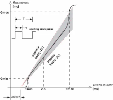
reproduces the EFI operating condition better. It is the fuel flow delivered when the EFI is pulsed with an electrical signal, usually measured in milliseconds. This flow is usually given in milligrams per pulse, or grams per 1,000 pulses. The duration of the pulse must be given. Fig. 3 shows graphically these two definitions. It is important to point out that the value of the static flow coincides with that obtained by the slope of the dynamic flow line.
axis) and to adjust the spring loading (preset) of the armature by means of a locking screw until the desired flow is obtained at that point. The spring loading adjusts the opening and closing time of an EFI, but it does not affect the static flow.
According to DeGrace-Bata (1985) and Garret (1990), during the operation of an EFI, the electromechanic interactions promote significant delays (as that between the instant when the exciting pulse begins and the instant at which the EFI begins releasing the fuel; or as the delay between the finish of the exciting pulse and the moment at which the EFI stops releasing fuel). The delays promote a displacement of the point where the fuel flow is zero in relation to the origin of the time pulse width axis (Fig. 3) creating the appearance of a “dead zone ” popularly known as offset .
In agreement with Garret (1990), for an electronic control meter the fuel supply to the engine with precision, there must be a linear relationship between the quantity of fuel delivered, Q and the pulse width applied, Wҏover the full delivery range. As DeGrace-Bata (1985) say, linearity is usually expressed in terms of the lowest pulse width or fuel flow at which Flow vs. Input Pulse Width lies on a straight line within a specified percentage of the theoretical flow (Fig. 3). About this there is not a strict consensus: according to Toyoda et al. (1982) the EFI linearity should stay within ±2%. De Grace-Bata (1985) are more tolerant and extend this tolerance to ±2.5%. Matsubara et al.(1986) prefer using ±1.5%. For this article, the criterion of ±2% was adopted. Linearity in the smallest pulses is specially important because, as Greiner et al. (1987) say, the increasing use of injection in smaller engines demands high
metering accuracy with minimal pulse times. This in turn requires minimizing injector opening and closing times. Linearity of injection improves with both the ratio of the actuation force to the mass of the delivery valve (armature) and the appropriate matching with it of the electrical and time constants of the solenoid circuit. Since the time required to close the injector is a function of the current in the solenoid at the point at which its circuit is broken, delivery errors are difficult to avoid when the pulse width is shorter than that necessary for the solenoid current to reach a stable value.
The dynamic range is defined as the ratio of maximum to minimum duration of injection (Fig. 3). Garrett (1990) defines the
minimum linear duration of injection, Qmin, as the difference
between the shortest linear pulse width and the offset. In order to maximize the dynamic range, EFI makers fight to keep Qmin as small
as practicable because the minimum duration of injection is determined to a major degree by injector design and the consequent offset of the delivery characteristics (Garret, 1990). So, it can be said that the moving mass affects directly Qmin. Matsubara et al.
(1986) affirm that reducing the armature weight and a higher spring preset load are effective to get wide dynamic control range. On the other hand, Garret (1990) says that the maximum duration of injection,Qmax, is primarily a function of the rotational speed of the
engine and whether the EFI is fired once or twice per revolution. Because of the non linear flow characteristics at both ends, the EFI can be utilized only between Qmin e Qmax where linearity is within
the tolerance adopted, whatever it is (Toyoda et al., 1982).
yoke
coil
adjustment mechanism seat
armature
return spring
stop metering section
terminals
outlet
power
inlet
needle
seat section
Figure 1. A set of 3 EFIs (pointed by the light arrow) mounted at an intake manifold. An EFI injects fuel directly into the intake valve.
331 Figure 3. A characteristic curve of an EFI: Fuel Flow x Time Pulse Width.
Nomenclature
B = spring’s damping coefficient
F = force
j = -1
Ks = spring’s stiffness elasture coefficient
M = armature’s mass
q = ratio M·Ks/B
2
Q = mass fuel flow
s = Laplace’s complex variable
t = time
T = period between exciting pulses
x = armature’s displacement Zn = undamped natural frequency
W = exciting pulse width that is applied to the EFI ’s solenoid coil
] = damping ratio
Index
min = minimum
mag = magnetic
max = maximum
ss = steady state
Modelling the EFI’s Mechanical System
As mentioned above, the way an EFI functions is relatively simple, however the complexity of the mathematical description of the physical actions and of the equations involved is considerable. Several forces and effects appear and disappear during the EFI functioning as, for example, a shock between the armature and the valve seat during the closure of the EFI or a shock between the armature and the limiter at the end of the course during the EFI opening. If some effects are not significant at some times, at other times they contribute significantly. Authors like Smith-Spinweber (1980), Karidis-Turns (1982), MacBain (1985), Kushida (1985), Pawlack-Nehl (1988), Lesquesne (1990a), Yuan-Chen (1990), Kawase-Ohdachi (1991), Ohdachi et al. (1991), Kajima (1992 and 1993), Passarini (1993), Rahman et al. (1996), Ando et al. (2001), Szente-Vad (2001) and Passarini-Pinotti Jr. (2003) diverge when describing the armature movement of the of the EFI and as to which of the above mentioned phenomena should be considered and which
should be neglected. It seems that most of these authors consider it sufficient to calculate precisely the magnetic force attraction, Fmagto
accurately define the armature movement because basically their mathematical model is described by only three forces, magnetic, elastic (Hook’s law) and viscous as shown in Eq. (1):
x . B x . K F x .
M mag s (1)
For a more complete discussion on modelling an EFI’s mechanical system, please refer to Passarini-Pinotti Jr. (2003). In this article this traditional basically linear mass-spring-damper (MKsB) governed by Eq. (1) and represented in Fig.4 was adopted because:
Figure 4. Linear MKsB model adopted to analyze the EFI mechanical system.
a) it allows the use of Laplace’s transforms and consequently, the application of the root-locus method (very much used in the analysis of linear systems);
b) even when such a complete and sophisticated model is not used, the chosen model supplies satisfactory results [because only a part of the problem is studied: that in which the non-linearities are small. It will be shown latter that the simulation done with a much more complex and complete model (Passarini, 1993) has confirmed the results obtained with this simpler approach ].
By hypothesis it was assumed that all elements are pure and ideal. The characteristic equation of a MKsB system is shown in Eq. (2):
Ms2BsKs 0. (2)
The actual spring exhibits the characteristics illustrated in the graph of Fig.5. The linearized model was obtained according to Passarini (1993) and the parameters Ks and B were found.
Analysis of the Problem
The root-locus method is very powerful in the dynamic analysis of linear systems (Ogata, 1993). Applying it to the characteristic equation Eq. (2), the influence of M on the transient response of the MKsB system could be investigated. For convenience, the ratio q
was defined as:
q M Ks
Figure 5. Elastic characteristic of the spring used in the EFI prototype montage.
Figure 6 shows the root-locus drawn as a function of the ratio q. It can be verified that:
1. MKsB systems with very large moving mass (q » 0.25) oscillate very much and are sluggish. Therefore ,they are not appropriate for application in this case.
2. MKsB systems with very small moving mass (q« 0.25) do not oscillate, however, when excessively decreasing the moving mass, i. e. qo 0, will not bring any significant gain either on the system time constant or response speed of the
system #Ks
B §
© ·¹, due to the influence of the pole located at
s Ks
B. Therefore, this dismantles the previous idea: “the smaller the magnitude of the moving mass, the better”. 3. The best response and therefore, the best adjustment of M
appears to occur when the roots are produced close to the
breakaway point on the real axis located ats 2Ks
B (whenq= 0.25). The MKsB system exhibits a behavior that is practically non-oscillatory and will still have one of the smallest setting times possible.
Confirming the Results Obtained with the MKsB
Root-Locus
To confirm the result obtained with the root-locus method, the dynamic impulsive response of the MKsB system was used to analyze the system performance. This analysis of the impulsive response is quite useful because it represents very well the system behavior under impacts.
Figure 6. The MKsB system root-locus as a function of the ratio q.
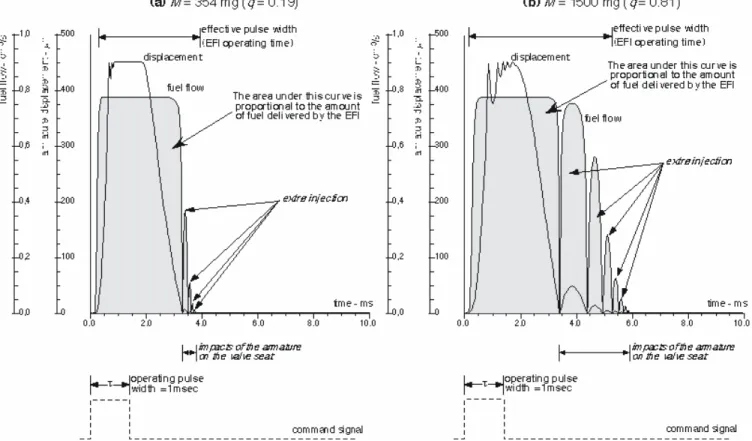
When an EFI is opening or closing its armature collides several times against the stopper or against the valve seat, respectively, over and over again until all the mechanic energy present in it is dissipated (please, refer to Fig. 7). This phenomenon is known as armature bounce or rebound. Although rebounds also happen at the shocks of the armature with the stop, its influence is important only when the moving mass is very large, i. e., when q >0.75.
While the armature rebounds one or more times, some amount of released fuel is affected, mainly during the closing of the EFI (please refer again to Fig. 7). The surrounding medium and the presence of vibrations introduce randomness to the rebound of the armature. For that reason, the shocks are not uniform but randomly and so, its influence on the fuel flow is not systematic as was thought. This fact contributes to decrease the EFI linearity and repeatability, mainly during operation under short pulse widths. In fact, DeGrace-Bata (1986) affirm that the main cause for deviations of the linearity in short pulse widths are the variations at the opening and closing times. These authors observed that:
1) .significant flow linearity errors can be found even at a pulse width beyond the time when the armature is fully open and the armature bounce has subsided, and
2) this flow non-linearity can be directly correlated to closing of the armature alone (i.e., opening times are not affected). In fact, the simulation shown in Fig. 7 confirmed this last observation.
In order to improve this EFI transient response the criterion used was, by taking a impulsive response of a MKsB system with null mass as reference, to determine the instant when 99% of its mechanical energy was dissipated. It was found that this instant corresponds to t# 2.3·B/Ks. After this, the dissipated power within
this period of time was computed for the range 0 < q< 2. The graph is shown in Fig.8. It can be noticed that out of the area in which
333 Figure 7. EFI’s time response: armature displacement and the corresponding instantaneous fuel flow versus time (W = 1 msec and T = 9 msec). (a) M = 354 mg (q = 0.19), (b) M = 1500 mg (q = 0.81). Notice that in the fuel flow curve (b) shown at right. The exceeding amount of released fuel is almost exclusively due to the armature bouncing against the valve seat. In addition to this, observe how the EFI operation time jumps from ~3,5 msec to ~6,0 msec.
Results:
All the previous theoretical analysis led us to obtain the following results:
Figure 8. Dissipated power graph (compared to the MKsB system when
M = 0) as a function of ratio q. The detail shows the root-locus with the roots that produced the indicated landing.
1) the root locus method pointed to an optimum ratio qoptimum
close to 0.25;
2) a refinement came when examining the dissipation of the mechanical energy present in the MKsB system relative to the KsB (when M= 0). This criterion revealed a qoptimum=
0.21. It could be considered that 0.20 < qoptimum< 0.23 since
at this range the power dissipation curve stays practically constant and closely to 100%.
Verification of the Results
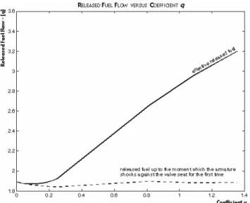
Figure 9. The fuel released by the EFI up to the instant that the armature touches the valve seat is practically constant, however systems with large moving mass have more difficulty in dissipating all the mechanical energy at the stopping shock. Because of the successive armature shocks against the valve seat, some extra quantity of fuel is released promoting the loss of accuracy of the EFI and consequently a loss of linearity.
The following Table 1 shows the physical characteristics of the studied prototype.
Table 1. Some characteristics of the EFI prototype.
Coil Characteristics
xexcitation pulse (voltage mode) xelectrical resistance
xinductance
xcopper wire diameter (AWG) xnumber of coil turns
11.88 V x 1 msec 0.9348 (ohms)
0.5057 (mH) 0.4 (AWG 26)
225
Mechanical Characteristics
xreturn spring
xspring coefficient (Ks) xdamping coefficient (B) xsurrounding medium xmaterial (armature and yoke)
3313 (N/m) 2,47 (Ns/m) kerosene SAE 405
Figure 10. Verification of the influence of the armature mass on linearity (when Wҏ= 1 ms and T = 9 ms).
Conclusions
From the above results, it can be concluded that:
1) the adopted linear MKsB model was relatively suitable to analyze the physical problem, even though it is known that an EFI is complex and exhibits several non-linearities; 2) significant flow non-linearity that can be directly correlated
to closing of the armature alone can be significantly reduced if the choice of moving mass and return spring characteristics respects the following relationship:
0.2 MKs B2 0.23
This guarantees that the dissipation of power will be effective improving the EFI linearity at shorter pulses. Another consequence is that the EFI operation time is relatively reduced (please, refer to Fig. 7) and so, the EFI dynamic range is increased. This is particularly interesting for those who want to build up an injection strategy.
Although the exciting pulse is frequently related to the released fuel flow, it is significantly shorter than the EFI operation time as it could be seen at Fig. 7. It means that the engine control system designer should keep in mind that as the available time for fuel injection is a function of the rotational speed. At high engine speed conditions, this difference could become critical and some transient problems, as engine instability or poor transient response, could prejudice the engine performance.
Acknowledgment
We would like to register our gratefulness to FAPESP for the financial support given to our IC project, process n.97/08142-4.
References
Ando, R.; Koizumi, M.; Ishikawa, T., 2001, “Development of a Simulation Method for Dynamic Characteristics of Fuel Injector”, IEEE Transactions on Magnetics, v. 37, n. 5, pp. 3715-3718.
DeGrace, L. G., Bata G.T., 1985, “The Bendix DEKA Fuel Injector Series-Design and Performance” SAE Technical Papers Series, n. 850559 (SP-609), pp. 57-63.
Garret, K., 1990, “Petrol Injector and Exhaust Catalyst Developments”, Automotive Engineer, v. 15, n. 3, pp. 62-63.
Greiner, M., Romann, P., Steinbrenner, U., 1987, “Injectors Developments Examined”, Automotive Engineering, v. 95 n. 2, pp. 43-47.
Kajima, T., 1993, “Development of a High-Speed Solenoid Valve: Investigation of the Energizing Circuits”, IEEE Transactions on Industrial Electronics, v. 40, n. 4, pp. 428-435.
Kajima, T.; Kawamura, Y., 1995, “Development of a High-Speed Solenoid Valve: Investigation of Solenoids”, IEEE Transactions on Industrial Electronics, v. 42, n. 1, pp. 1-8.
Kajima, T.; Nakamura, Y.; Sonoda, K., 1992, “Development of a High-Speed Solenoid Valve: Investigation of the Energizing Circuits”, Proceedings of the 1992 International Conference on Industrial Electronics, Control, Instrumentation and Automation ”, v. 01, pp. 564-569.
Karidis, J.P., Turns, S.R., 1982, “Fast-acting Electromagnetic Actuators: Computer Model Development and Verification”, SAE Technical Papers Series, n. 820202, pp. 11-25.
Kawase, Y.; Ohdachi, Y., 1991, “Dynamic Analysis of Automotive Solenoid Valve Using Finite Element Method”, IEEE Transactions on Magnetics, New York, v. MAG-27, n. 5, pp.3939-3942.
Kushida, T., 1985, “High Speed Powerful and Simple Solenoid Actuator “DISOLE” and Its Dynamic Analysis Results”, SAE Technical Papers Series, n. 8503763, pp.3. 127-3.136.
335 Lesquesne, B., 1990b, “Fast-acting, Long-stroke Solenoids With Two
Springs”, IEEE Transactions on Industry Applications, New York, v. 26, n. 5, pp. 848-856.
MacBain, J.A., 1985, “Solenoid Simulation With Mechanical Motion”, International Journal for Numerical Methods in Engineering, New York, v. 21, pp. 13-18.
Matsubara, M., Ando, T., Takada, S., Takeuchi, H., 1986 “Aisan Fuel Injector for Multipoint Injection System”, SAE Technical Papers Series, n. 860486, pp. 125-130.
Passarini, L.C., 1993, “Análise e Projeto de Válvulas Eletromagnéticas Injetoras de Combustível: Uma Nova Proposta”, Doctoral thesis, Universidade de São Paulo, EESC, São Carlos-SP, Brasil.
Passarini, L.C.; Pinotti Jr., M., 2003, “A New Model for Fast Acting Electromagnetic Fuel Injector Analisys and Design”, Journal of the Brazilian Society of Mechanical Sciences, v.25, n. 3, pp.97-108.
Pawlack, A.M.; Nehl, T.W., 1988, “Transient Finite Modelling of Solenoid Actuators: the Coupled Power Electronics, Mechanical, and Magnetic Field Problem”, IEEE Transactions on Magnetics, v. MAG-24, n. 1, pp. 270-273.
Ohdachi, Y.; Kawase, Y.; Murakami, Y.; Inaguma, Y., 1991, “Optimum Design of Dynamic Response in Automotive Solenoid Valve”, IEEE Transactions on Magnetics, v. 27, n. 6, pp. 5226-5228.
Ogata, K., 1993, “Engenharia de Controle Moderno”, 2a.Ed., Editora Prentice/Hall do Brasil, Rio de Janeiro, Brasil.
Rahman, M.F.; Cheung, N.C.; Lim, K.W., 1995, “Position Estimation in Solenoid Actuators”, Conference Record of the 1995 IEEE Thirtieth IAS Annual Meeting (IAS ’95), 1995 Industry Applications Conference, v. 1, pp. 476-483.
Szente, V.; Vad, J., 2001, “Computational and Experimental Investigation on Solenoid Valve Dynamics”, Proceedings 2001 IEEE/ASME International Conference on Advanced Intelligent Mechatronics, v. 1, pp. 618-623.
Toyoda, T., Inoue, T., Aoki, K., 1982, “Single Point Electronic Injection System” SAE Technical Papers Series, n. 820902, pp. 83-87.