SIMPLE AND WEAK
∆
-INVARIANT POLYHEDRAL SETS FOR
DISCRETE-TIME SINGULAR SYSTEMS
Eugênio B. Castelan
∗Sophie Tarbouriech
†∗DAS / CTC / UFSC, Departamento de Automação e Sistemas, 88.040-900 - Florianópolis (S.C.), Brazil
†LAAS - CNRS, 7, Avenue du Colonel Roche, 31077 – Toulouse Cedex 4, France
ABSTRACT
In this paper, necessary and sufficient conditions for the positive invariance of convex polyhedra with respect to lin-ear discrete-time singular systems subject to bounded addi-tive disturbances are established. New notions of ∆-invari-ance under different assumptions on the initial conditions are defined. Specifically, the notions of simple and weak ∆-invariance are considered. They can be seen as extensions of the∆-positive invariance concept used for the regular lin-ear systems with additive disturbances. The results are pre-sented by considering classical equivalent system represen-tations for linear singular systems.
KEYWORDS: Singular systems, Disturbances, Convex poly-hedra, Invariance, Initial conditions.
RESUMO
Apresentam-se condições necessárias e suficientes para a in-variância positiva de poliédros convexos relativamente a um sistema singular, linear e em tempo discreto, sujeito a per-turbações aditivas e limitadas. Introduz-se as noções de ∆-invariância simples e de∆-invariância fraca, associadas a di-ferentes hipóteses a serem verificadas pelas condições ini-ciais. Estas noções podem ser consideradas como exten-sões, para o caso de sistemas singulares, do conceito de ∆-invariância utilizado no caso de sistemas regulares sujeitos
Artigo submetido em 20/12/2000
1a. Revisão em 10/9/2002; 2a. Revisão 30/4/2003 Aceito sob recomendação do Ed. Assoc. Prof. Liu Hsu
a perturbações. Os resultados são desenvolvidos a partir de duas formas usuais de representação de sistemas singulares lineares.
PALAVRAS-CHAVE: Sistemas singulares, Perturbações, Po-liédros convexos, Invariância, Condições iniciais.
1
INTRODUCTION
The use of the positive invariance property in the control of constrained dynamical systems has been receiving much at-tention in the last years (Blanchini, 1990; Blanchini, 1994; De Santis, 1994; Georgiou and Krikelis, 1991; Gilbert and Tan, 1991; Hennet, 1989; Hennet and Béziat, 1991; Kol-manovski and Gilbert, 1995; Milani and Dórea, 1996; Tar-bouriech and Gomes da Silva Jr., 1997; TarTar-bouriech and Castelan, 1993; Tarbouriech and Castelan, 1995). This prop-erty is used, for instance, to guarantee the maintenance of the state trajectories of a controlled system in the interior of some prescribed sets of admissible states determined from some sets of control or state constraints. External disturbances and/or parametric perturbations can also be considered. The positive invariance in presence of disturbances is commonly referred in the literature as∆-invariance (Blanchini, 1990; De Santis, 1994; Kolmanovski and Gilbert, 1995).
in the considered model.
The objective of this paper is to present necessary and suf-ficient algebraic conditions to guarantee the positive invari-ance property of convex polyhedra with respect to singu-lar discrete-time systems subject to additive disturbances belonging to a convex set ∆. The general notion of ∆-invariance of a domainD ⊂ ℜnwith respect to a dynamical system is associated to the maintenance of the system trajec-tories within the domainDfor any initial condition belong-ing toDand for any sequence of admissible disturbances be-longing to∆. Thus, a major objective of this paper consists in extending the∆-invariance concept used for the regular linear systems to the linear singular systems.
Due to the specificities of singular systems in terms of initial conditions (initial conditions may be consistent or not), some different notions have to be considered. Hence, from the as-sumptions on the initial conditions with respect to the domain
D, we define the notions of simple and weak∆-invariance.
Considering convex polyhedra, the algebraic characteriza-tion of both the simple and weak∆-invariance properties are obtained for an equivalent representation of special interest in the theory of linear singular systems, called Differential-Algebraic Form.
The paper is organized as follows. The problem to be treated and the simple and weak∆-invariance properties are formu-lated in section 2. Section 3 presents the main results in terms of the Differential-Algebraic Representation. Some general comments about the proposed results are given in section 4. An illustrative example in section 5 allows to show an appli-cation of the results to a constrained control problem. Section 6 ends the paper with some concluding remarks.
2
PROBLEM PRESENTATION
Consider a linear discrete-time singular perturbed system de-scribed by:
Exk+1=A0xk+Dwk (1) whereE ∈ ℜn×n withrank(E) = q ≤ n, A
0 ∈ ℜn×n,
D ∈ ℜn×d. x
k ∈ ℜn andwk ∈ ℜd represent respectively the state and additive disturbance vectors. System (1) can, for instance, represent the closed-loop dynamic behavior of a linear singular system
Exk+1=Axk+Buk+Dwk (2)
controlled by a static full state feedback or static output feedback. In these cases, we have A0 = A + BF or
A0=A+BKC, respectively.
Since for control purposes system (1) represents controlled systems, we shall consider that it has a unique solution for
all initial conditionx0∈ ℜnand for any admissible sequence {wk}, with wk ∈ ℜd, ∀k ≥ 0, and also that the system is causal. Thus, the following assumption is supposed to hold throughout this note (for details see, for instance, Dai (1989) and Lewis (1986)).
Assumption 1 The pair(E, A0) is assumed to be regular
and system (1) is supposed to be impulse free.
However, the dynamic behavior of system (1) can present discontinuous behavior atk= 0if the associated initial con-ditionx0 is not consistent. For any given initial condition
x0, the actual state atk= 0is denotedxk|k=0 =x0+. The
set of consistent initial conditions (Dai, 1989) is the set ofx0
which prevents the system of discontinuous behavior:
I0={x0∈ ℜn;x0+=x0} (3)
It is well-known that in the case of the unperturbed system (wk = 0,∀k),I0corresponds to the subspace ofℜnspanned
by the finite eigenvectors of the pair(E, A0). But, in the case
of system (1),I0depends also onw0. In general, ifw0= 0,
a finite jump with amplitude|x0−x0+|may occur atk= 0 for any initial conditionx0.
Thus, let us now introduce different notions of∆-invariance depending on certain assumptions made about the initial con-ditions. The first definition is the closest to the practical situ-ation of hard constraints.
Definition 1 A nonempty set D ⊂ ℜn is a simple ∆-invariant domain with respect to system (1) if for any ini-tial conditionx0 ∈ D and sequence{wk}, withwk ∈ ∆, ∀k≥0, it follows thatx0+∈ Dandxk∈ D,∀k≥1.
The second definition is weaker in terms of hypothesis be-cause it assumes that only the initial condition x0 belongs
to the invariant domain. It may be used, for instance, in practical situations of soft constraints or, as indicated by the comments in section 4, for stability and disturbance rejection purposes.
Definition 2 A nonempty setD ⊂ ℜnis a weak∆-invariant domain with respect to system (1) if for any initial condition
x0∈ Dand sequence{wk}, withwk∈∆,∀k≥0, it follows thatxk ∈ D,∀k≥1.
In this work, we are mainly concerned with the application of Definitions 1 and 2 to the case of closed polyhedral domains. In practical control problems, polyhedral domains can repre-sent linear constraints on the state and limits for the allowed disturbances. The polyhedral sets of states and disturbances to be considered in the sequel are defined by:
R(G, ρ) ={x∈ ℜn;
Gx≤ρ}, G∈ ℜg×n, ρ∈ ℜg (4)
and
∆ =R(T, µ) ={w∈ ℜd;
T w ≤µ}, T ∈ ℜp×d, µ∈ ℜp (5) Any nonempty convex polyhedron ofℜnorℜpcan be char-acterized by (4) or (5), respectively. By convention the in-equalities between vectors are component-wise.
Thus, the primary objective of this work is to give alge-braic necessary and sufficient conditions for both the simple and weakR(T, µ)-invariance of convex polyhedronR(G, ρ) with respect to system (1). To accomplish the stated objec-tives, we shall consider an equivalent representation of sys-tem (1), called Differential-Algebraic form, and the corre-sponding representation of the polyhedral setR(G, ρ). An-other particular equivalent representation of system (1), un-der a Standard form, is also used in the proofs of the proposed results.
In general, an equivalent representation of system (1) can be obtained as follows (see Dai (1989)). Let Q˜ andP˜ be two nonsingularn-order matrices. Then, by considering the change of coordinatesx= ˜Px˜, the following equivalent rep-resentation of system (1) can be defined:
˜
Ex˜k+1= ˜A0x˜k+ ˜Dwk (6)
where: E˜ = ˜QEP˜, A˜0 = ˜QA0P˜, and D˜ = ˜QD. The
corresponding representation of the polyhedral setR(G, ρ)is given by:R( ˜G, ρ) ={x˜∈ ℜn; ˜Gx˜≤ρ}, withG˜=GP .˜
3
MAIN RESULTS
Sincerank(E) = q, there exist nonsingularn-order matri-cesQ =
Q′
1
Q′
2
andP =
P1 P2 such thatQEP =
Iq 0 0 0
(Dai, 1989). Thus, by considering the change of
coordinates x =
P1 P2
x1 x2
, with x1 ∈ ℜq and
x2∈ ℜ(n−q), system (1) can be rewritten as
Iq 0 0 0
x1
k+1
x2
k+1
=
A1 A2
A3 A4
x1
k
x2
k
+
D1
D2
wk (7)
where:QA0P =
A1 A2
A3 A4
, QD=
D1
D2
, with
A1∈ ℜq×q, A2∈ ℜq×(n−q), A3∈ ℜ(n−q)×q,
A4∈ ℜ(n−q)×(n−q), D1∈ ℜq×d, D2∈ ℜ(n−q)×d.
Since the singular system is supposed to be impulse free, ma-trixA4is nonsingular (Dai, 1989; Lewis, 1986). The
corre-sponding representation of the polyhedronR(G, ρ)is given by
R(G1, G2, ρ) =
x1
x2
∈ ℜn
;
G1G2
x1
x2
≤ρ
(8) where:G1=GP1∈ ℜg×qandG2=GP2∈ ℜg×(n−q).
The equivalent representation (7) gives a good meaning to singular systems: the system is composed of dynamic sub-systems and an algebraic part which represents the connec-tion between subsystems. Thus, descripconnec-tions of dynamical systems under the Differential-Algebraic Form arise natu-rally when systems are formed from interconnected systems (Dai, 1989). Otherwise, a representation of any linear singu-lar system under the form (7) can be generally obtained from a singular value decomposition of matrixE(Dai, 1989).
The following result presents necessary and sufficient alge-braic conditions for the simple∆-invariance property of con-vex polyhedra.
Proposition 1 The polyhedral set R(G1, G2, ρ) is simply
R(T, µ)-invariant with respect to system (7) if and only if there exist nonnegative matrices S1 ∈ ℜg×g,S2 ∈ ℜg×p,
S3 ∈ ℜg×p,S4 ∈ ℜg×g,S5 ∈ ℜg×p andS6 ∈ ℜg×p such
that:
S1G¯1 = G¯1(A1−A2A−41A3) (9)
S1G¯2 = 0 (10)
S2T = G¯1(D1−A2A−41D2) (11)
S3T = −G¯2A−41D2 (12)
S4G¯1 = G¯1 (13)
S4G¯2 = 0 (14)
S5T = −G¯2A−41D2 (15)
S6T = 0 (16)
S1ρ+ (S2+S3)µ ≤ ρ (17)
S4ρ+ (S5+S6)µ ≤ ρ (18)
where, by definition:G¯1=G1−G2A4−1A3andG¯2=G2.
Proof: To develop the proof, we shall represent the
subsystems related, respectively, to the finite and in-finite eigenvalues of the (impulse free) singular sys-tem (Dai, 1989). Thus, by considering the
nonsingu-lar n-order matrices Q¯ =
Iq −A2A−41
0 A−41
, P¯ =
¯
P1 P¯2 =
Iq 0 −A−41A3 In−q
and the change of
co-ordinates x1 x2 = ¯
P1 P¯2
¯ x1 ¯ x2
, system (7) can be
rewritten as
Iq 0 0 0 ¯ x1 k+1 ¯ x2 k+1 = ¯
A1 0
0 In−q ¯ x1 k ¯ x2 k + ¯ D1 ¯ D2 wk (19) where: ¯
A1 = (A1 −A2A−41A3), D¯1 = (D1−A2A−41D2) and
¯
D2=A−41D2.
The corresponding representation of the polyhedronR(G, ρ) is given by
R( ¯G1,G¯2, ρ) =
¯ x1 ¯ x2
∈ ℜn; ¯
G1G¯2
¯ x1 ¯ x2 ≤ρ (20)
Notice that with respect to system (19), we always havex¯2k = −D¯2wk,∀k. In particular, ifk= 0and an initial condition ¯
x0 =
¯
x10
¯
x20
is considered, it follows that the actual
sub-statex¯2
k|k=0 = −D¯2w0 and, hence, x¯0+ =
¯
x1 0 −D¯2w0
.
Thus, in general a jump occurs atk= 0, which is now con-sidered.
>From Definition 1, the simple R(T, µ)-invariance of
R( ¯G1,G¯2, ρ)with respect to system (19) corresponds to:
¯
G1 G¯2
¯ x1 k+1 ¯ x2 k+1 ≤ρ and ¯
G1 0 −G¯2D¯2
¯
x1k
¯
x2k wk
≤ρ
for all
¯
x1k ¯
x2
k
andwksuch that
¯
G1 G¯2 0
0 0 T
¯ x1 k ¯ x2 k wk ≤ ρ µ (21)
From (19), this condition also writes:
¯
G1A¯1 0 G¯1D¯1 −G¯2D¯2
¯
G1 0 −G¯2D¯2 0
¯
x1k ¯
x2k
wk
wk+1
≤ ρ ρ for all ¯
x1k ¯
x2k
,wkandwk+1such that
¯
G1 G¯2 0 0
0 0 T 0
0 0 0 T
¯
x1k
¯
x2k
wk
wk+1
≤ ρ µ µ .
By using the extended Farkas’ lemma (Hennet, 1989), it fol-lows that a necessary and sufficient condition for the weak ∆-invariance ofR( ¯G1,G¯2, ρ)is the existence of a
nonnega-tive matrix
S1 S2 S3
S4 S5 S6
satisfying both:
S1 S2 S3
S4 S5 S6
¯
G1 G¯2 0 0
0 0 T 0
0 0 0 T
=
¯
G1A¯1 0 G¯1D¯1 −G¯2D¯2
¯
G1 0 −G¯2D¯2 0
and
S1 S2 S3
S4 S5 S6
ρ µ µ ≤ ρ ρ .
Therefore relations (9)-(18) of Proposition 1 follow. ✷
Relative to the weak∆-invariance property we get the fol-lowing result.
Proposition 2 The polyhedral setR(G1, G2, ρ) is weakly
R(T, µ)-invariant with respect to system (7) if and only if there exist nonnegative matricesW1 ∈ ℜg×g,W2 ∈ ℜg×p
andW3∈ ℜg×psuch that
W1G¯1 = G¯1(A1−A2A−41A3) (22)
W1G¯2 = 0 (23)
W2T = G¯1(D1−A2A−41D2)(24)
W3T = −G¯2A−41D2 (25)
W1ρ+ (W2+W3)µ ≤ ρ (26)
where, by definition:G¯1=G1−G2A4−1A3andG¯2=G2.
Proof: As in the previous proof, the standard form (19) is
used to obtain the desired invariance relations. From Def-inition 2, a necessary and sufficient condition for the weak
R(T, µ)-invariance ofR( ¯G1,G¯2, ρ)with respect to system
(19) is
¯
G1 G¯2
¯ x1 k+1 ¯ x2 k+1
≤ρ (27)
for all ¯ x1 k ¯ x2 k
andwksuch that
¯
G1 G¯2 0
0 0 T
¯
x1k ¯
x2k
For all x¯k ∈ R( ¯G1,G¯2, ρ) and for all admissible
distur-banceswk ∈R(T, µ),∀k, one can also write:
¯
G1 G¯2 0 0
0 0 T 0
0 0 0 T
¯
x1
k ¯
x2
k
wk
wk+1
≤
ρ µ µ
(29)
In the same way, since from (19) we getx¯2
k+1=−D¯2wk+1,
(27) is equivalent to
¯
G1A¯1 0 G¯1D¯1 −G¯2D¯2
¯
x1k
¯
x2k wk
wk+1
≤ρ (30)
Hence the weak R(T, µ)-invariance of R( ¯G1,G¯2, ρ),
ex-pressed by (27) and (28), is obtained when every solution of (29) is also solution of (30), which corresponds to the in-clusion of a polyhedral convex set into another polyhedral convex set. Then by applying the extended Farkas’ lemma (Hennet, 1989), it follows that a necessary and sufficient con-dition for the weak∆-invariance ofR( ¯G1,G¯2, ρ)is the
exis-tence of a nonnegative matrix W1 W2 W3 satisfying
both:
W1 W2 W3
¯
G1 G¯2 0 0
0 0 T 0
0 0 0 T
=
¯
G1A¯1 0 G¯1D¯1 −G¯2D¯2
and
W1 W2 W3
ρ µ µ
≤ρ .
Therefore, relations (22)-(26) of Proposition 2 follow. ✷
We finish this section with the following remarks related to the Standard form (19). By recalling the general procedure described in section 2 to obtain an equivalent representation (6), we first remark that (19) can be obtained from (1) by con-sideringQ˜ =QQ¯,P˜ =PP¯and the change of coordinates
x = ˜Px˜, wherex˜ =
¯
x1
¯
x2
. Next, let us recall that the
finite eigenvalues of the considered regular and impulse-free singular system are given by the zeros of the characteristic polynomial
det(λE−A0) =det
˜
Q−1
λIq−A¯1 0
0 In−q
˜
P−1
.
Thus, theqfinite eigenvalues of pair(E, A0)correspond to
the eigenvalues of matrixA¯1∈ ℜq×qthat are the roots of the
characteristic equation (Kailath, 1980):
det
λIq−(A1−A2A−41A3)= 0.
4
GENERAL COMMENTS
The concept of∆-invariance reduces to the classical concept of positive invariance in the case of unperturbed (regular and impulse free) singular systemExk+1=A0xk. Hence, alge-braic characterizations of the positive invariance property of
R(G, ρ), as presented by Tarbouriech and Castelan (1993), can be easily obtained from Propositions 1 and 2 by consid-eringD= 0,T = 0andµ= 0.
The case of regular linear systems can be viewed as a partic-ular case of system (19), by considering only the slow sub-system
¯
x1k+1= ¯A1x¯1k+ ¯D1wk (31) Thus, the classicalR(T, µ)-invariance ofR( ¯G1, ρ)with
re-spect to system (31) can be characterized by using Proposi-tion 2 withG¯2= 0,D¯2= 0andW3= 0.
Furthermore, notice that no assumption on the signs of the elements of vectorsρandµis considered in the presented results. However, in most control applications the zero-state has to be feasible and we can consider that both vectorsρand
µare nonnegative, that is,ρ∈ ℜg+andµ∈ ℜd+, whereℜ
g
+
(resp.ℜd
+) denotes the positive orthant ofℜg(resp.ℜd).
Under the assumption of non-negativeness ofρandµ, some stability properties of the eigenvalues of matrix W1 can
be deduced from relation (26) by using the theory of non-negative matrices andM-matrices (Tarbouriech and Caste-lan, 1993). Thus, relation (22) can be thought as expressing a certain intersection between the spectra ofW1andA¯1;
re-lation (23) implies the existence of some null eigenvalues in the spectrum ofW1. According to this intersection, some
sta-bility properties of the singular system can be deduced since its set of finite eigenvalues is given by the spectrum ofA¯1
(Tarbouriech and Castelan, 1993).
As shown by Milani and Dórea (1996), the existence of admissible matrices W2 and W3 satisfying relations
(24)-(25) is related to the following null-space intersections: ¯
D1Ker(T) ⊆ Ker( ¯G1)and−D¯2Ker(T) ⊆ Ker( ¯G2).
Also, consider both the set of relations (9)-(18) of Propo-sition 1 and (22)-(26) of PropoPropo-sition 2. It is clear that the conditions of Proposition 1 are harder to satisfy than those of Proposition 2. If relations (9)-(18) hold then relations (22)-(26) also hold forW1 =S1,W2 = S2,W3 =S3. Hence,
ifR(G, ρ)is a simple R(T, µ)-invariant domain, then it is also a weakR(T, µ)-invariant domain, but the converse is not generally true. Therefore relative toR(G, ρ)the follow-ing implication holds :
simpleR(T, µ)-invariant ⇒weakR(T, µ)-invariant.
the initial condition x0 belongs to D, whereas the notion
of simple∆-invariance requires that both the initial condi-tionx0and the associated discontinuous statex0+belong to
D. However, a particular case exists where the two studied notions of∆-invariance become equivalent. This case oc-curs wheneverR( ¯G1,G¯2, ρ)is unbounded in the directions
of sub-statex¯2. In such a case, we necessarily haveG2 =
¯
G2= 0and it means that any jump due to non-consistent
ini-tial condition is admitted. Thus, ifR(G1, ρ) =R(G1,0, ρ)
is a weakR(T, µ)-invariant set it is also a simpleR(T, µ )-invariant set. This can also be verified from the conditions of Propositions 1 and 2.
Since the singular system can describe a kind of intercon-nected system, its sub-statex¯2can be considered as a pseudo-state andx¯20represents the interconnection between
subsys-tems at initial time k = 0 (Dai, 1989). In this context, non-consistent initial conditions would represent topological changes in the interconnections’ level. Therefore, in practi-cal situations, both the choice of matrixG¯2 = G2and the
used ∆-invariance concept (simple and/or weak) has to be associated to the possible topological changes in the inter-connections between subsystems.
5
ILLUSTRATIVE EXAMPLE
Consider the open-loop discrete-time singular system (2) borrowed from (Tarbouriech and Castelan, 1993), described by the following matrices:
E=
1 0 0 0 1 0 0 0 0
, A=
1.2 0 0
−1 −0.7 −1 2 −0.5 −1.2
, B= 0 1
1 −1 0.5 2
, D= 0 1 1 (32)
The set R(T, µ) of allowed persistent disturbances is de-scribed by T = 1 −1
; µ=γ
1 1
(33)
whereγis some positive scalar.
The vector of admissible controls is constrained to belong to a compact setΩ
Ω ={uk ∈ ℜm; −̺≤uk≤̺} ; ̺= ̺1 ̺2 > 0 0 (34) Thus, assuming that a saturated state-feedback control law is applied
uk =sat(F xk) (35)
wheresat(ui) = sign(ui) min{|ui|, ̺i},fori = 1,2, the
closed-loop system is given by:
Exk+1=Axk+Bsat(F xk) +Dwk (36)
This closed-loop system is non-linear but, for any statexk inside the polyhedral setS(F, ̺), defined from Ωby (37), the state atk+ 1is determined by the linear model (2):
S(F, ̺) ={xk∈ ℜn; −̺≤F xk ≤̺} (37)
Let us now consider the state feedback matrixF ∈ ℜ2×3
computed by Tarbouriech and Castelan (1993):
F =
F1
F2 =
0 1
−1 0
0.9318
−0.1164
(38)
The corresponding closed-loop linear model under the form (1) is determined by matricesEandDgiven before and by:
1 0 0 0 1 0 0 0 0
xk+1=
0.2 0.0 −0.1164 0.0 0.3 0.0481 0.0 0.0 −0.9668
xk+ 0 1 1
ωk
(39)
Since the corresponding setS(F, ̺)is not an invariant do-main with respect to (39), saturations may occur for trajec-tories emanating fromS(F, ̺). Hence, one can be interested in verifying the invariance property in the presence of distur-bances from some subset ofS(F, ̺). In this way, we are pri-marily interested in verifying theR(T, µ)-invariance prop-erty of the setR(G, ρ) defined in (4), whereG andρ are given by: G=
0 1 0.9318
−1 0 −0.1164
0 0 1
0 −1 −0.9318 1 0 0.1164
0 0 −1
, ρ= 1 2 1 1 2 1 .
Notice that the considered setR(G, ρ)verifiesR(G, ρ) ⊆
S(F, ̺). In the unperturbed case (wk = 0, ∀k), the set
R(G, ρ)is a weak positively invariant set of system (39). In the perturbed case, the objective is to determine the maxi-mal scalarγ =γmaxsuch thatR(G, ρ)is weaklyR(T, µ
)-invariant with respect to (39). By using Linear Program-ming to evaluate the relations of Proposition 2, we obtain
γmax= 0.208815with:
W1=
0.3000 0.0 0.0000 0.0000 0.0 0.2795 0.7632 0.2 0.0232 0.7632 0.0 0.0000 0.0000 0.0 0.0000 0.0000 0.0 0.0000 0.0000 0.0 0.2795 0.3000 0.0 0.0000 0.0000 0.0 0.0000 0.0000 0.2 0.0232 0.0000 0.0 0.0000 0.0000 0.0 0.0000
W2=
1.0497 0.0000 0.1203 0.0000 0.0000 0.0000 0.0000 1.0497 0.0000 0.1203 0.0000 0.0000
, W3=
0.9637 0.0000 0.0000 0.1203 1.0343 0.0000 0.0000 0.9637 0.1203 0.0000 0.0000 1.0343
.
Let us now consider the polyhedral setR( ˆG,ρˆ), where:
ˆ
G=
F1 0 −F1 0
=
0 1 0
−1 0 0
0 −1 0 1 0 0
, ρˆ=
1 2 1 2
.
This set corresponds to the intersection R(G, ρ) ∩ I0,
whereI0 is the set of consistent initial conditions of
sys-tem (39) in the unperturbed case. Since bothR(G, ρ)and
I0are invariant domains with respect to (39), the unbounded
setR( ˆG,ρˆ)is also an invariant domain in the disturbance-free case (Tarbouriech and Castelan, 1993). In the per-turbed case, it can be verified thatR( ˆG,ρˆ)is both simply and weakly R(T, µ)-invariant with respect to system (39), for γ = ˆγmax = 0.6667. In particular, the following
ma-trices can be used to verify the relations of Proposition 2:
ˆ W1=
0.3 0.0 0.0 0.0 0.0 0.2 0.0 0.0 0.0 0.0 0.3 0.0 0.0 0.0 0.0 0.2
,
ˆ W2=
1.0497 0.0000 0.1203 0.0000 0.0000 1.0497 0.0000 0.1203
andWˆ3= 0.
Let us now show some system trajectories emanating from the above considered∆-invariant sets. To simplify the anal-ysis, we shall consider that the control bounds, represented by the elements of̺ >0, are sufficiently large so that no sat-urations occur, i.e., any considered trajectory evolves inside
S(F, ρ)and is determined by the linear model (39).
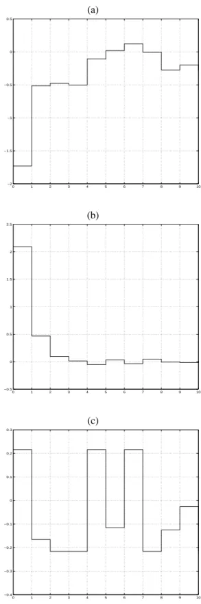
Fig.1 shows the time-response of the first three components of vectorGxk(due to symmetry property) by considering the setR(G, ρ)andγmax = 0.208815. The considered
distur-bances are randomly generated so that the corresponding se-quencewkbelongs to the interval[−γmax, γmax]. By
choos-ing the initial conditionx0 = −2.1164 −1.9318 1 ′,
one getsx0+ = −2.1164 −1.9318 0.2160 ′
. Notice thatGx0 ≤ρwhereasGx0+ ≤ρ. But, sinceR(G, ρ)is a
weakR(T, µ)-invariant set, one getsGxk≤ρ,∀k≥1.
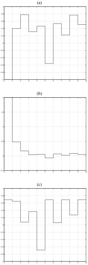
Fig.2 shows the time-response of the first two components of vector Gxˆ k (due to symmetry property) and the time-response of the last component of vector xk by consider-ing the setR(G, ρ) ∩ I0andγmax = 0.6667. By
choos-ing the initial conditionx0 = −2 −1 0
′
, one gets
x0+ =
2 1 0.6896 ′. Notice that bothGxˆ 0 ≤ ρand
ˆ
Gx0+ ≤ρ.
(a)
0 1 2 3 4 5 6 7 8 9 10
−2 −1.5 −1 −0.5 0 0.5
(b)
0 1 2 3 4 5 6 7 8 9 10
−0.5 0 0.5 1 1.5 2 2.5
(c)
0 1 2 3 4 5 6 7 8 9 10
−0.4 −0.3 −0.2 −0.1 0 0.1 0.2 0.3
(a)
0 1 2 3 4 5 6 7 8 9 10
−1 −0.8 −0.6 −0.4 −0.2 0 0.2 0.4 0.6 0.8 1
(b)
0 1 2 3 4 5 6 7 8 9 10
−0.5 0 0.5 1 1.5 2
(c)
0 1 2 3 4 5 6 7 8 9 10
−1 −0.8 −0.6 −0.4 −0.2 0 0.2 0.4 0.6 0.8 1
Figure 2: (a)-(b).Time-response of the first two components ofGxˆ k. (c). Time-response of the last component ofxk
.
6
CONCLUSION
We have presented some results on the invariance property of convex polyhedra with respect to linear singular systems with additive disturbances. In this way, we have defined the notions of simple and weak∆-invariance according to the assumptions on the initial conditions. Algebraic necessary and sufficient conditions for characterizing these properties have been proposed relative to two classical equivalent sys-tem representations.
As for regular systems, the presented results may be used for solving constrained control problems (Castelan and Tar-bouriech, 1996). To this end, the computation of the maxi-mal admissible weakly∆-invariant set contained in a given polyhedron of constraints is considered in Tarbouriech and Castelan (1997). Finally, we remark that a similar technique can be proposed to compute the maximal simply∆-invariant set.
ACKNOWLEDGEMENTS
This work has been partially supported by CNPq (Brazil) and CNRS (France). The authors would like to thank the review-ers for their comments and suggestions.
REFERENCES
Blanchini, F. (1990). Feedback control for linear time-invariant systems with state and control bounds in the presence of disturbances, IEEE Transactions on
Auto-matic Control 35(11): 1231–1234.
Blanchini, F. (1994). Ultimate boundedness control for un-certain discrete-time systems via set-induced lyapunov functions, IEEE Transactions on Automatic Control
39(2): 428–433.
Castelan, E. B. and Tarbouriech, S. (1996). Positively invari-ant sets for discrete-time singular systems with additive perturbations, Proc. of 36th IEEE-CDC, Kobe (Japan), pp. 992–993.
Castelan, E. B. and Tarbouriech, S. (2000). Weak and strong ∆-invariant polyhedral sets for discrete-time singular systems, Anais do XIII Congresso Brasileiro de
Au-tomática (CBA 2000), Florianópolis (Brazil).
Dai, L. (1989). Singular Control System, Springer-Verlag.
De Santis, E. (1994). On positively invariant sets for discrete-time linear systems with disturbance: an application of maximal disturbance sets, IEEE Transactions on
Georgiou, G. and Krikelis, N. J. (1991). A design approach for constrained regulation in discrete singular systems,
System & Control Letters 17: 297–304.
Gilbert, E. G. and Tan, K. T. (1991). Linear systems with state and control constraints : the theory and application of maximal output admissible sets, IEEE Transactions
on Automatic Control 36(9): 1008–1020.
Hennet, J. C. (1989). Une extension du lemme de farkas et son application au problème de régulation linéaire sous contraintes, C. R. Acad. Sci. Paris 308(I): 415–419.
Hennet, J. C. and Béziat, J. P. (1991). A class of invariant regulators for the discrete-time linear constrained regu-lation problem, Automatica 27(3): 549–554.
Kailath, T. (1980). Linear Systems, Prentice-Hall, Engle-wood Cliffs, NJ.
Kolmanovski, I. and Gilbert, E. G. (1995). Maximal out-put admissible sets for discrete-time systems with dis-turbance inputs, Proc. of ACC 1995, Seattle (USA), pp. 1995–1999.
Lewis, F. L. (1986). A survey of linear singular systems,
Circuits Systems Signal Process 5(1): 3–36.
Milani, B. E. A. and Dórea, C. E. T. (1996). On invariant polyhedra of continuous-time systems subject to addi-tive disturbances, Automatica 35(5): 785–789.
Tarbouriech, S. and Castelan, E. B. (1993). On positively invariant sets for singular discrete-time systems,
Inter-national Journal Systems Science 24(9): 1687–1705.
Tarbouriech, S. and Castelan, E. B. (1995). An eigenstructure assignment approach for constrained linear continuous-time systems, System & Control Letters 24: 333–343.
Tarbouriech, S. and Castelan, E. B. (1997). Maximal admis-sible polyhedral sets for discrete-time singular systems with additive disturbances, Proc. of 37th IEEE-CDC, San Diego (USA), pp. V.4, 3164–3169.